Quantitative Modeling and Analytical Calculation
of Elasticity in Cloud Computing
Keqin Li ,
Fellow, IEEE
Abstract—Elasticity is a fundamental feature of cloud computing and can be considered as a great advantage and a key benefit of cloud computing. One key challenge in cloud elasticity is lack of consensus on a quantifiable, measurable, observable, and calculable definition of elasticity and systematic approaches to modeling, quantifying, analyzing, and predicting elasticity. Another key challenge in cloud computing is lack of effective ways for prediction and optimization of performance and cost in an elastic cloud platform. The present paper makes the following significant contributions. First, we present a new, quantitative, and formal definition of elasticity in cloud computing, i.e., the probability that the computing resources provided by a cloud platform match the current workload. Our definition is applicable to any cloud platform and can be easily measured and monitored. Furthermore, we develop an analytical model to study elasticity by treating a cloud platform as a queueing system, and use a continuous-time Markov chain (CTMC) model to precisely calculate the elasticity value of a cloud platform by using an analytical and numerical method based on just a few parameters, namely, the task arrival rate, the service rate, the virtual machine start-up and shut-down rates. In addition, we formally define auto-scaling schemes and point out that our model and method can be easily extended to handle arbitrarily sophisticated auto-scaling schemes. Second, we apply our model and method to predict many other important properties of an elastic cloud computing system, such as average task response time, throughput, quality of service, average number of VMs, average number of busy VMs, utilization, cost, cost-performance ratio, productivity, and scalability. In fact, from a cloud consumer’s point of view, these performance and cost metrics are even more important than the elasticity metric. Our study in this paper has two significance. On one hand, a cloud service provider can predict its performance and cost guarantee using the results developed in this paper. On the other hand, a cloud service provider can optimize its elastic scaling scheme to deliver the best cost-performance ratio. To the best of our knowledge, this is the first paper that analytically and comprehensively studies elasticity, performance, and cost in cloud computing. Our model and method significantly contribute to the understanding of cloud elasticity and management of elastic cloud computing systems.
Index Terms—Cloud computing, continuous-time Markov chain, cost-performance ratio, elasticity, queueing model
Ç
1
I
NTRODUCTION1.1 Challenges and Motivations 1.1.1 Elasticity Characterization
C
LOUD computing is a paradigm for enabling ubiqui-tous, convenient, and on-demand network accesses to a shared pool of configurable computing resources (e.g., servers, storage, networks, data, software, applications, and services), that can be rapidly provisioned and released with minimal management effort or service provider interaction [32]. The unique and essential characteristics of cloud com-puting include on-demand self-service, broad and variety of network access, resource pooling and sharing, rapid elas-ticity, measured and metered service. Among these fea-tures, elasticity is a fundamental and key feature of cloud computing, which can be considered as a great advantage and a key benefit of cloud computing, and perhaps what distinguishes this new computing paradigm from other ones, such as cluster and grid computing [14].The Merriam-Webster dictionary defines elasticity as the capability of a strained body to recover its size and shape
after deformation. Its synonyms include stretchiness, flexi-bility, pliancy, suppleness, plasticity, resilience, springiness, sponginess, and adaptability. In physics, elasticity (from Greek"astikothta, “elastikotita”) is the tendency of solid materials to return to their original shape after being deformed. A solid object will deform when forces are applied on it. If the material is elastic, the object will return to its initial status (e.g., shape and size) when these forces are removed. A cloud computing platform is like a solid object. The resource (e.g., virtual machines (VMs)) utilization and quality of service (QoS, e.g., the average task response time) are properties and status of the platform. The dynamic work-load (e.g., the number of service requests) changes are ex-ternal forces. When the workload increases (decreases, respectively), the resource utilization increases (decreases, respectively), and the service quality decreases (increases, respectively), e.g., the average task response time increases (decreases, respectively), i.e., the cloud computing platform is deformed. To return to its original status, the platform should have the capability to adjust itself, e.g., increasing (decreasing, respectively) the number of VMs, so that both resource utilization and quality of service can return to their original status. Notice that the above definition of elasticity is only qualitative, but not quantitative. The most important problem in studying cloud elasticity is the apparent lack of a quantifiable, measurable, and observable definition of elas-ticity in cloud computing, and thus no approach to analyzing
The author is with the Department of Computer Science, State University of New York, New Paltz, NY 12561 USA. E-mail: [email protected]. Manuscript received 31 Jan. 2016; revised 28 Dec. 2016; accepted 2 Feb. 2017. Date of publication 7 Feb. 2017; date of current version 3 Dec. 2020. Recommended for acceptance by M. Parashar, O. Rana, and R.C.H. Hsu. Digital Object Identifier no. 10.1109/TCC.2017.2665549
2168-7161ß2017 IEEE. Personal use is permitted, but republication/redistribution requires IEEE permission. See ht_tps://www.ieee.org/publications/rights/index.html for more information.
and predicting elasticity has been well developed so far, although several researchers have attempted to characterize cloud elasticity (see Section 2.1). Such a definition allows for the creation of analytical models and methods that not only calculate elasticity, but also enable deployment, manage-ment, improvemanage-ment, and enhancement of cloud computing platforms.
In economics, elasticity is the measurement of how res-ponsive an economic variable is to a change in another. In particular, elasticity can be quantified as the ratio of the per-centage change in one variable to the perper-centage change in another variable. Using this definition, elasticity in cloud computing can be defined as how the amount of computing resource changes as the current workload changes. It seems that the definition is quantitative and measurable; however, such a definition of responsiveness is not entirely adequate, since it only considers how much, not how fast, the comput-ing resource adapts. If a cloud computcomput-ing platform takes a long time to provide the correct amount of resources to match the workload (which might not be current any more), it is not considered as elastic. The time required to restore the original status, so that the provided computing resour-ces match the current workload, should be taken into account. Elasticity (i.e., the ability to dynamically acquire or release computing resources in response to variable demand) is meaningful to the cloud users only when the acquired VMs can be provisioned in time and ready to use within the user expectation. The long unexpected VM start-up time could result in resource under-provisioning, which will inevitably hurt system performance [30]. Similarly, the long unexpected VM shut-down time could result in ource over-provisioning, which will inevitably hurt res-ource utilization.
1.1.2 Performance and Cost Optimization
In addition to the issues mentioned above, existing studies of elasticity mostly focused on characterizing elasticity, but emphasized much less from users’ point of view. Customers of cloud services only care high quality of service and low cost of service, and do not care whether such quality and cost are supported by elasticity. Therefore, the ultimate pur-pose of elasticity is to benefit the users, although such elastic management of a cloud computing platform is transparent to users and applications. All efforts in studying elasticity should be incorporated into performance and cost control, management, prediction, and optimization.
Elasticity research should help in the following two ways.
Performance and cost predictability—The analytical models and methods developed for measuring elas-ticity should help to make the performance and cost of a cloud computing platform predictable, manage-able, and improvable.
Auto-scaling scheme optimality—The models and methods should also be able to guide the construc-tion, optimizaconstruc-tion, and comparison of auto-scaling schemes for the best interest of the users of an elastic cloud computing platform.
Unfortunately, the above challenges have not been well investigated in the existing literature.
1.2 Contributions of the Paper
As mentioned above, one key challenge in cloud elasticity is lack of consensus on a quantifiable, measurable, observable, and calculable definition of elasticity and systematic app-roaches to modeling, quantifying, analyzing, and predicting elasticity. Another key challenge in cloud computing is lack of effective ways for prediction and optimization of perfor-mance and cost in an elastic cloud platform. The main objec-tive of this paper is to address these two pressing issues.
Our contributions in this paper can be summarized as follows.
First, we present a new, quantitative, and formal definition of elasticity in cloud computing, i.e., the probability that the computing resources provided by a cloud platform match the current workload. Our definition is applicable to any cloud platform and can be easily measured and monitored. Further-more, we develop an analytical model to study elasticity by treating a cloud platform as a queueing system, and use a con-tinuous-time Markov chain (CTMC) model to precisely calcu-late the elasticity value of a cloud platform by using an analytical and numerical method based on just a few parame-ters, namely, the task arrival rate, the service rate, the virtual machine start-up and shut-down rates. In addition, we for-mally define auto-scaling schemes and point out that our model and method can be easily extended to handle arbi-trarily sophisticated scaling schemes.
Second, we apply our model and method to predict many other important properties of an elastic cloud com-puting system, such as average task response time, through-put, quality of service, average number of VMs, average number of busy VMs, utilization, cost, cost-performance ratio, productivity, and scalability. In fact, from a cloud con-sumer’s point of view, these performance and cost metrics are even more important than the elasticity metric. Our study in this paper has two significance. On one hand, a cloud service provider can predict its performance and cost guarantee using the results developed in this paper. On the other hand, a cloud service provider can optimize its elastic scaling scheme to deliver the best cost-performance ratio. We also show that an elastic platform can consume less resources, achieve shorter average task response time, pro-vide the same performance guarantee with higher probabil-ity, and have less cost and lower cost-performance ratio than an inelastic platform.
To the best of our knowledge, this is the first paper that analytically and comprehensively studies elasticity, perfor-mance, and cost in cloud computing. Our model and method significantly contribute to the understanding of cloud elasticity and management of elastic cloud computing systems.
2
R
ELATEDR
ESEARCHIn this section, we review four areas related to our study, i.e., cloud elasticity characterization, elastic cloud comput-ing system development, cloud platform modelcomput-ing and analysis, and elastic system performance assessment. 2.1 Characterizing Cloud Elasticity
Several researchers have attempted to characterize cloud elasticity. These definitions are classified into two
categories. The first category includes those definitions which are only qualitative, but not quantitative. In [5], elas-ticity is defined as the ability for customers to quickly request, receive, and later release as many resources as needed. Elastic computing has the feature of dynamic varia-tion in the use of computer resources to meet a varying workload [7]. In [20], elasticity is defined as the degree to which a system is able to adapt to workload changes by pro-visioning and depropro-visioning resources in an autonomic manner, such that at each point in time the available resour-ces match the current demand as closely as possible. In [27], elasticity is the feature of automated, dynamic, flexible, and frequent resizing of resources that are provided to an appli-cation by the execution platform. However, all these charac-terizations are not quantified.
The second category includes those definitions which are quantitative, but not analytically tractable. Some attempts have been made to propose a quantitative and measurable definition of cloud elasticity. It is mentioned in [27] that a unified (single-valued) metric for elasticity could possibly be achieved by a combination of three characteristics, namely, reconfiguration effect (i.e., the amount of added/ removed resources, expressing the granularity of adapta-tion), reconfiguration frequency (i.e., the density of reconfig-uration points over a time period), and reconfigreconfig-uration time (i.e., the time interval between the instant when a reconfigu-ration has been triggered/requested and the instant when the adaptation has been completed), in such a way that the elasticity metric is in the range of½0;1. Although each of the above three properties can be observed and measured, there is no specific equation or formula given in [27] for such a single-valued elasticity metric. In [20], an elasticity metric for scaling up (down, respectively) is defined in such a way that it is inversely proportional to the product of the average time to switch from an under-provisioned (over-provi-sioned, respectively) state to a normal state, which corre-sponds to the average speed of scaling up (down, respectively), and the average amount of under-provisioned (over-provisioned, respectively) resources during an under-provisioned (over-under-provisioned, respectively) period. Since theoretically, the speed of scaling can be arbitrarily fast, the above definition can possibly lead to an “infinitely elastic” cloud computing system. Furthermore, although each of the above two properties can be monitored and measured, there is no given method to predict, e.g., the average amount of under-provisioned or over-provisioned resources, and therefore, there is no way to obtain elasticity analytically. In [22], a definition of elasticity was given, which relates elas-ticity with over-provisioning and under-provisioning penal-ties. However, the amounts of over-provisioning and under-provisioning are only observable, but not analytically avail-able and predictavail-able.
Some other efforts have also been made to study elastic-ity. In [12], elasticity properties have been considered in terms of cost elasticity (i.e., the responsiveness of resource provision to changes in cost) and quality elasticity (i.e., the responsiveness of quality to changes in resource usage). In [14], elastic systems are classified in terms of four character-istics, i.e., scope (infrastructure, application, platform), pol-icy (manual, reactive, predictive), purpose (performance, capacity, cost, energy), and method (replication, resizing,
migration). In [37], application elasticity is considered, i.e., making an application automatically adjust to variations in load without the need of intervention of a human adminis-trator and without the need to change its code.
2.2 Developing Elastic Computing Systems
In [8], the authors described a platform for developing scal-able applications on the cloud by QoS-driven resource pro-visioning from different sources and supporting different and elastic applications. In [11], the authors considered elas-tic VMs for rapid and optimal virtualized resources alloca-tion. In [13], the authors presented an elastic web hosting provider, that makes use of the outsourcing technique in order to take advantage of cloud computing infrastructures for providing scalability and high availability capabilities to the web applications. In [18], the authors presented a novel predictive elastic resource scaling scheme for cloud systems, which unobtrusively extracts fine-grained dynamic patterns in application resource demands and adjusts their resource allocation automatically. In the context of cloud computing, auto-scaling mechanisms hold the promise of assuring QoS properties for applications, while simultaneously making efficient use of resources and keeping operational costs low for the service providers. In [34], the authors developed a model-predictive algorithm for workload forecasting that is used for resource auto-scaling. In [35], the authors devel-oped a cost-aware system that provides efficient support for elasticity in the cloud by (i) leveraging multiple mechanisms to reduce the time to transition to new configurations, and (ii) optimizing the selection of a virtual server configuration that minimizes the cost. Elastic resource scaling allows cloud systems to meet application service-level agreements (SLA) with minimum resource provisioning costs. In [36], the authors presented a system that automates fine-grained elastic resource scaling for multi-tenant cloud computing infrastructures.
In [1], the authors presented a service-oriented dynamic resource management model, which covers the issues of resource prediction, customer type-based resource estima-tion and reservaestima-tion, advanced reservaestima-tion, pricing, refund-ing and acquired quality of service-based refundrefund-ing. In [2], the authors provided a holistic brokerage model to manage on-demand and advance service reservation, pricing, and reimbursement, with dynamic management of customer’s characteristics and historical record in evaluating the eco-nomics related factors.
2.3 Modeling Cloud Platforms
2.4 Assessing Elastic System Performance
(Due to space limitation, Sections 2.3 and 2.4 are moved to the supplementary file, which can be found on the Computer Society Digital Library at http://doi.ieeecomputersociety. org/10.1109/TCC.2017.2665549.)
3
D
EFINITION OFE
LASTICITYIn this section, we formally define cloud elasticity, and also compare the notion with several related concepts. For read-er’s convenience, we provide Table 1, which gives a sum-mary of notations and their definitions in the order introduced in the paper.
3.1 A New Definition
It has been clear based on our discussion so far that a defini-tion of elasticity in cloud computing should satisfy the fol-lowing two conditions.
Quantitative describability—the definition should be quantifiable, measurable, and observable, which is based on a few parameters and is formally defined based on a rigorous model.
Analytical tractability—the definition should be ana-lytically available, calculable, and predictable, which is easily obtained by using a simple, standard, and straightforward method.
We say that a cloud computing system is in (1) a normal state if the provided computing resources match the current workload; (2) an over-provisioning state if the provided computing resources exceed the current workload; (3) an under-provisioning state if the provided computing resour-ces cannot handle the current workload. Our definition of elasticity of a cloud computing platform with dynamically variable workload isthe percentage of time (or, the probability) that the system is in the normal state.
Formally, assume that a system is operating for a time period of lengthT. LetTnormal (Tover,Tunder, respectively) be the total time that the system is in the normal (over-provi-sioning, under-provi(over-provi-sioning, respectively) state. It is clear thatT ¼TnormalþToverþTunder. Then, the elasticity is calcu-lated as
E¼Tnormal T ¼1
ToverþTunder
T : (1)
If the system has been operating for a sufficiently long period of time and is in a stable state, then pnormal¼ Tnormal=T is the probability that the system is in the normal state,pover¼Tover=T is the probability that the system is in
the over-provisioning state, and punder¼Tunder=T is the probability that the system is in the under-provisioning state. Hence, we get
E¼pnormal¼1 ðpoverþpunderÞ: (2) Notice that our definition of elasticity in Eq. (1) is easily measurable and observable by monitoring a cloud comput-ing platform. Of course, the notions of normal, over-provi-sioning, and under-provisioning states still need to be quantified. Since our elasticity metric is defined quantita-tively as probability, its value is in the range½0;1. Analyti-cal tractability is impossible unless there is a rigorous mathematical model. We will present a queueing model for cloud platforms, define auto-scaling schemes, employ a CTMC model for elastic cloud platforms and quantitatively characterize our metric, and develop an analytical and numerical method to compute the proposed metric of Eq. (2), thus satisfying the two requirements mentioned ear-lier. It will also be clear that our elasticity metric depends on only a few (five, in particular) parameters.
It is also noticed that our definition of elasticity captures the three characteristics in [27], i.e., reconfiguration effect, reconfiguration frequency, and reconfiguration time, and the two characteristics in [20], i.e., the average time to switch and the average amount of under-provisioned or over-pro-visioned resources, where the reconfiguration effect and the average amount of under-provisioned or over-provisioned resources affect the definition of normal/over-provision-ing/under-provisioning states, and the reconfiguration fre-quency, the reconfiguration time, and the average time to switch are all reflected and summarized in E, i.e., Tover, Tunder,pover, andpunder.
3.2 Related Notions and Properties
There are several concepts which are related to (and some-times considered as similar to or even the same as) elastic-ity. In the following, we clarify the difference between these concepts and elasticity.
Resilience. In material science, resilience is the ability of a material to absorb energy when it is deformed elastically, and release that energy upon unloading. Resiliency is the persistence of service delivery that can justifiably be trusted when facing changes, which should be considered as differ-ent from fault-tolerance, reliability, availability, recoverabil-ity, and performability [15]. In [16], the authors quantified the resiliency of Infrastructure-as-a-Service (IaaS) clouds subject to changes in demand and available capacity, using a stochastic reward net based model for provisioning and servicing requests, with respect to two key performance measures, i.e., job rejection rate and provisioning response delay.
Scalability. Scalability is the ability of a system, network, or process to handle a growing amount of work in a capable manner or its ability to be enlarged to accommodate that growth. A scalable system improves its performance propor-tionally to the added capacity. Scalability has been a signifi-cant issue in parallel, distributed, cluster, grid, networked, and cloud computing systems. In [21], elastic scaling strate-gies are divided into three categories: (1) in and scale-out-strategies which allow adding more homogeneous TABLE 1
Summary of Notations and Definitions
Notation Definition
E elasticity
pnormal the probability in a normal state
pover the probability in an over-provisioning state
punder the probability in an under-provisioning state
m the number of active servers (i.e., VMs)
the task arrival rate m the service rate
k the number of tasks in the system ðm; kÞ a state
ðam; bmÞ a pair of integers defining different states
S an elastic cloud management and auto-scaling scheme a the VM start-up rate
b the VM shut-down rate
pðm; kÞ the equilibrium steady-state probability of stateðm; kÞ N the average number of tasks
T the average task response time
R the throughput
M the average number of servers
B the average number of busy servers
U the VM utilization r the server utilization
pk the probability that a queueing system is in statek
machine instances or processing nodes of the same type based on the agreed service-level agreement; (2) up and scale-down—strategies which are implemented by using more powerful machine instances or processing nodes with faster processors/cores and more memory and storage; (3) mixed scaling—strategies which allow one to scale up (or scaled own) and scale-out (or scale-in) computing resources in terms of quantity and quality at the same time. In [19], scale-in and scale-out are called horizontal scalability, and scale-up and scale-down are called vertical scalability. In [27], it was men-tioned that scalability includes application scalability (i.e., a property which means that an application maintains its per-formance goals and service-level agreement even when its workload increases) and platform scalability (i.e., the ability of a cloud platform to provide as many resources as needed by an application). In [28], the technique of using workload dependent dynamic power management (i.e., variable power and speed of processor cores according to the current work-load, which is essentially vertical scalability) to improve sys-tem performance and to reduce energy consumption is investigated by using a queueing model.
4
A
NALYTICALM
ODEL ANDM
ETHODIn this section, we present our analytical model and method to compute the proposed elasticity value.
4.1 A Queueing Model
A cloud computing platform is a multiserver system which has m identical servers (i.e., VMs). In this paper, a multi-server system is treated as an M/M/m queueing system which is elaborated as follows [26]. There is a Poisson stream of service requests (i.e., tasks) with arrival rate (measured by the number of service requests that are sub-mitted in one unit of time), i.e., the inter-arrival times are independent and identically distributed (i.i.d.) exponential random variables with mean 1=. A multiserver system maintains a queue with infinite capacity for waiting tasks when all themservers are busy. The first-come-first-served (FCFS) queueing discipline is adopted. The task execution times are i.i.d. exponential random variables with mean
1=m. The m servers are homogeneous and have identical execution and service rate m(measured by the number of tasks that can be finished in one unit of time).
Notice that in an elastic cloud computing platform, the number of servers adapts to the current workload (i.e., the number of tasks in the system). Therefore, we have a multi-server queuing system with a variable number of multi-servers, and an elastic cloud computing platform is no longer an M/ M/m queueing system. In [4], the authors dealt with a mul-tiserver retrial queueing model in which the number of active servers depends on the number of customers in the system. The servers are switched on and off according to a multithreshold strategy. For a fixed choice of the threshold levels, the stationary distribution and various performance measures of the system are calculated. In [23], a multiserver Poisson queuing system with losses and a variable number of servers was investigated, and all major characteristics of the system were obtained in an explicit form. Unfortunately, these results are not directly applicable to elastic cloud com-puting systems, because the times to turn on and off the
servers are not considered. However, as mentioned before, these factors are critical in measuring elasticity, and must be included into our queueing model.
4.2 Auto-Scaling Scheme
We useðm; kÞto denote astate, wherem1is the number of active servers, andk0is the number of tasks in the sys-tem. Letðam; bmÞ,m1, be a pair of integers used to
deter-mine the status of a state, where bm > amm1,
amþ1bm, for all m1, and a1 < a2 < a3 < , b1 < b2 < b3 < . An elastic cloud platform management and auto-scaling scheme can be represented as
S¼ ðða1; b1Þ;ða2; b2Þ;. . .;ðam; bmÞ;. . .Þ; (3)
which decides how a cloud computing platform responds to the workload change. States are classified into three types.
A state is anover-provisioningstate if0kam.
A state is anormalstate ifam < kbm.
A state is anunder-provisioningstate ifk > bm.
The number of a servers can be adjusted according to the status of the state. In particular, a new server can be added (i.e., a cloud server system is scaled-out) if the current state is under-provisioning, and an active server can be removed (i.e., a cloud server system is scaled-in) if the current state is over-provisioning.
4.3 A Continuous-Time Markov Chain
To take the virtual machine start-up and shut-down times into consideration, we make the following assumptions. (1) A new server can be added as an active server at any time, and the time to initialize a new server is an exponential ran-dom variable with mean1=a(i.e., the VM start-up rate isa, measured by the number of VMs which can be initialized in one unit of time). (2) An active server can be removed at any time, and the time to finalize an active server is an expo-nential random variable with mean1=b(i.e., the VM shut-down rate isb, measured by the number of VMs which can be finalized in one unit of time).
Based on the above assumptions, it is clear that a multi-server system with variable and dynamically adjustable number of servers can be modeled by a continuous-time Markov chain (CTMC).
Our CTMC is actually a mixture of the birth-death pro-cesses similar to those for M/M/m queueing systems, with m1. The transitions among the states are described as fol-lows. (Note: We use the notationðm1; k1Þ !
r
ðm2; k2Þto rep-resent a transition from stateðm1; k1Þto stateðm2; k2Þ with transition rater.)
ðm; kÞ ! ðm; kþ1Þ, m1, k0. This transition happens when a new task arrives.
ðm; kÞ !mmðm; k1Þ, m1, k > am. This transition
happens when a task is completed, and the state
ðm; kÞis normal or under-provisioning.
ðm; kÞminðm!1;kÞmðm; k1Þ, m1, 1kam. This
transition happens when a task is completed, and the state ðm; kÞ is over-provisioning. (The value m1
means that a server is being shut down and not serv-ing, but is still in the system. A deactivated server is also a resource until it is removed from the system.)
ðm; kÞ !a ðmþ1; kÞ, m1, k > bm. This transition
happens when the stateðm; kÞis under-provisioning, and a new server is activated to join service.
ðm; kÞ !b ðm1; kÞ, m2, 1kam. This
transi-tion happens when the stateðm; kÞis over-provision-ing, and an active server is being shut down and removed from further service.
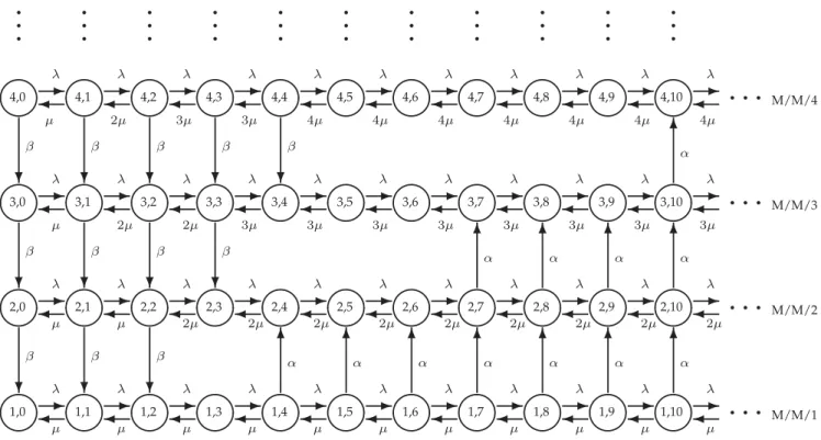
Fig. 1 shows a state-transition-rate diagram, assuming that am¼m and bm¼3m for all m1. The states in the
diagram are arranged in a two dimensional way, where each row of states is similar to the state-transition-rate dia-gram of an M/M/m queueing system, with the difference that the number of servers is m1 (not m) when m1kam due to the VM which is being shut down.
Notice that in a stateðm; kÞwherekbmþ1, a new VM is
activated and initialized, where the start-up time is an expo-nential random variable. It is possible that before the initiali-zation is completed, a task arrives or departs, and the state becomesðm; k1Þ. Since the residual start-up time has the same distribution as the original exponential distribution due to the memoryless property, the transition rate from
ðm; k1Þ to ðmþ1; k1Þ is still a. Similarly, in a state
ðm; kÞwhere kam, one VM is deactivated and finalized,
where the shut-down time is an exponential random vari-able. It is possible that before the finalization is completed, a task arrives or departs, and the state becomes ðm; k1Þ. Due to the memoryless property, the transition rate from
ðm; k1Þtoðm1; k1Þis stillb.
To summarize, our CTMC model for an elastic cloud com-puting system with variable number of virtual machines con-tains the following parameters:,m,a,b, and of course,S. It is worth to mention that the purpose of our research is to cap-ture the most essential parameters for elasticity quantifica-tion and predicquantifica-tion. Our model and method are by no means perfect, but only some initial attempt towards this direction. In a real cloud platform, things can be much more
complicated. First, there could be many components in resource management, such as physical machines, storage, and network resources. Second, there could be many factors (other than VM start-up and shut-down times) which affect VM creation and termination. However, it is clear that con-sidering all these factors and facts might result in infeasible modeling and analysis, although they could be included and considered in further investigation. For the purpose of feasi-ble modeling and analysis, our abstract model and analytical method are simplistic and manageable.
4.4 An Analytical and Numerical Method
Letpðm; kÞdenote the equilibrium steady-state probability that a multiserver system is in stateðm; kÞ. Unfortunately, there is no closed-form expression of pðm; kÞ. However, a numerical solution can be easily obtained by solving a linear system of equations resulted from our CTMC model using any standard method from linear algebra.
Once thepðm; kÞ’s are available, we can compute the elas-ticity metric as follows. The probability that the system is in the over-provisioning state is
pover¼ X1 m¼1 Xam k¼0 pðm; kÞ: (4) The probability that the system is in the under-provisioning state is punder¼ X1 m¼1 X1 k¼bmþ1 pðm; kÞ: (5) The probability that the system is in the normal state is
pnormal¼ X1 m¼1 Xbm k¼amþ1 pðm; kÞ: (6) Fig. 1. A state-transition-rate diagram.
Based on the above probabilities, our elasticity metric can be obtained by using Eq. (2).
4.5 Impact of the Basic Parameters
It is clear that by using the CTMC model to calculate the elasticity value of a cloud platform, our elasticity metric is determined by only a few parameters, namely, the task arrival rate, the service rate, the virtual machine start-up and shut-down rates, and the scaling scheme. In this sec-tion, we present numerical data to demonstrate the impact of these basic parameters on elasticity.
In Figs. 2, 3, 4, and 5, we assume that am¼m and
bm¼3mfor allm1.
Varying the Task Arrival Rate. In Fig. 2, we show pover, pnormal, and punder as functions of the task arrival rate , where m¼1, a¼2, b¼5, and ¼1:0;2:0;. . .;10:0. It is observed that asincreases,pover decreases (i.e., more ser-vice requests result in less probability of over-provisioning), and punder changes slightly (actually, increases and then decreases, i.e., more service requests result in slight change of the probability of under-provisioning), and pnormal increases (i.e., the elasticity increases).
Varying the Service Rate. In Fig. 3, we showpover,pnormal, and punder as functions of the task service rate m, where ¼5,a¼2,b¼5, andm¼1:0;2:0;. . .;10:0. It is observed that as mincreases, pover increases significantly (i.e., faster service rate results in greater probability of over-provision-ing), andpunderchanges noticeably (actually, increases and then decreases, i.e., faster service rate results in noticeable change of the probability of under-provisioning), andpnormal decreases significantly (i.e., the elasticity decreases significantly).
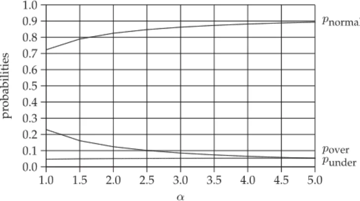
Varying the Virtual Machine Start-Up Rate. In Fig. 4, we show pover, pnormal, and punder as functions of the virtual machine start-up rate a, where ¼5, m¼1, b¼5, and
a¼1:0;1:5;. . .;5:0. It is observed that as a increases,pover increases slightly (i.e., faster virtual machine start-up rate results in greater probability of over-provisioning), and punderdecreases noticeably (i.e., faster virtual machine start-up rate results in noticeable reduction of the probability of under-provisioning), and pnormal increases noticeably (i.e., the elasticity increases noticeably).
Varying the Virtual Machine Shut-Down Rate. In Fig. 5, we show pover, pnormal, and punder as functions of the virtual machine shut-down rate b, where¼5,m¼1,a¼2, and
b¼5:0;5:5;. . .;10:0. It is observed that the impact of b is small. Asbincreases,poverdecreases slightly (i.e., faster vir-tual machine shut-down rate results in less probability of over-provisioning), andpunderincreases slightly (i.e., faster virtual machine shut-down rate results in greater probabil-ity of under-provisioning), and pnormal increases slightly (i.e., the elasticity increases slightly).
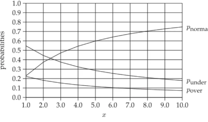
Varying the Scaling Scheme. In Fig. 6, we showpover,pnormal, andpunderas functions ofx, where¼5,m¼1,a¼2,b¼5, am¼m, andbm¼amþx, for allm1. It is observed that
the impact of the scaling scheme is big. Asxincreases (i.e., the interval ½am; bm gets wider), both pover and punder decrease noticeably (i.e., wider interval ½am; bm results in
less probability of over-provisioning and under-provision-ing), and pnormal increases significantly (i.e., the elasticity increases significantly).
It is worth to mention that the purpose of this section is to demonstrate the impact of some basic parameters on elastic-ity. These data are obtained based on our model and Fig. 2.pover,pnormal, andpunderversus.
Fig. 3.pover,pnormal, andpunderversusm.
Fig. 4.pover,pnormal, andpunderversusa.
method, and might not be entirely accurate for any real world use case scenario.
4.6 Simulation Results: Accuracy and Robustness To validate the accuracy and robustness of our CTMC model, we have performed extensive simulations and experiments. Our simulation environment is an Intel Xeon CPU E5620 2.40 GHz with the Linux OS version RHEL 6.8. The simulation program is written in C++ supported by the g++ 4.4.7 compiler. We simulate an elastic cloud computing platform with am¼m and bm¼3m for all m1, and
¼5,a¼2,b¼5, andm¼1:0;2:0;. . .;10:0. We (1) gener-ate a Poisson stream of service requests; (2) run the elastic cloud computing system; (3) recordTover,Tnormal, andTunder; (4) and report pover¼Tover=T, pnormal¼Tnormal=T, and punder¼Tunder=T, where T ¼TnormalþToverþTunder, until 1,000,000 service requests are completed.
In addition to the exponential distribution of task execu-tion times, we also consider several other distribuexecu-tions. The six probability distribution functions (pdf), all with the same expectation1=m, are described as follows.
Exponential distribution (EXP): The pdf ismemx.
Hyperexponential distribution (HEX): The pdf is w1m1em1xþw2m2em2xþw3m3em3x, wherew1¼0:2, w2¼0:3, w3¼0:5, m1¼y1m0, m2¼y2m0, m3¼y3m0, y1¼3, y1¼2, y1¼1, with m0¼mðw1=y1þw2=y2þ w3=y3Þ.
Erlang distribution (ERL): The pdf is m0em0x
ðm0xÞg1
=ðg1Þ!, wherem0¼gmandg¼5.
Hyper-Erlang distribution (HER): The pdf is w1m1em1xðm1xÞ g11 =ðg11Þ!þw2m2em2xðm2xÞ g21 = ðg21Þ!; where w1¼0:4, w2¼0:6, g1¼3, and g2¼4.
Uniform distribution (UNI): The pdf isðm=2Þ in the range½0;2=mÞ.
Pareto distribution (PAR): The pdf isaba=xaþ1in the range½b;1Þ, wherea¼2andb¼ ða1Þ=ðamÞ. In Table 2, we showpover,pnormal, andpunderas functions of the task service ratem, for all the above six probability distribution functions of task execution times, as well as the analytical results of our CTMC model. We have the following important observations. (1) Accuracy—The sim-ulation results for the exponential distribution are very close to the analytical results and validate the accuracy of our CTMC model. (2) Robustness—The simulation results for the hyperexponential distribution, Erlang distribution,
hyper-Erlang distribution, uniform distribution, and Par-eto distribution, especially the results ofpnormal, show the robustness of our CTMC model, i.e., the ability of the CTMC model to predict the elasticity E with reasonable accuracy even though some assumptions of our model are not satisfied.
4.7 Extension of the CTMC Model
The CTMC model can be extended to include more compli-cated scaling schemes.
Hot, Warm, and Cold VMs. It is known that physical machines (PMs) are categorized into three server pools: hot (i.e., with running VMs), warm (i.e., turned on but without running VM), and cold (i.e., turned off) [24]. Therefore, VMs can also be classified into three categories: hot (cur-rently running), warm (to be started up from a warm PM), and cold (to be started up from a cold PM). It is clear that a warm VM takes much less time to start than a cold VM. Let us assume that a cloud platform keeps certain numberm of hot and warm VMs and unlimited cold VMs. The warm VM and cold VM start-up rates area1 anda2respectively, wherea1 > a2. Then, we should haveðm; kÞ !
a1
ðmþ1; kÞ, for 1m < m and k > bm, and ðm; kÞ !
a2
ðmþ1; kÞ, for mm andk > bm. That is, the firstm VMs can be started
up faster than the remaining VMs. TABLE 2 Simulation Results
m ANA EXP HEX ERL HER UNI PAR
pover 1.0 0.05087 0.05191 0.05446 0.04341 0.04496 0.04519 0.04737 2.0 0.11458 0.12285 0.12707 0.10075 0.10337 0.10558 0.11159 3.0 0.20854 0.22145 0.22754 0.18933 0.19552 0.19574 0.21464 4.0 0.31983 0.33381 0.34003 0.30715 0.31158 0.30986 0.33752 5.0 0.43061 0.44184 0.44643 0.43138 0.43428 0.42806 0.46350 6.0 0.52955 0.53843 0.54011 0.54501 0.54548 0.53813 0.56954 7.0 0.61252 0.61893 0.61719 0.64157 0.63837 0.63090 0.65286 8.0 0.67979 0.68557 0.67847 0.71666 0.71034 0.70516 0.71685 9.0 0.73348 0.73698 0.72915 0.77327 0.76561 0.76218 0.76773 10.0 0.77617 0.77958 0.77202 0.81703 0.80887 0.80432 0.80550 pnormal 1.0 0.82503 0.82194 0.81342 0.84834 0.84524 0.84360 0.83649 2.0 0.68546 0.67416 0.66380 0.71782 0.71005 0.70516 0.69784 3.0 0.58055 0.56483 0.55639 0.61378 0.60477 0.60142 0.58623 4.0 0.49450 0.48026 0.47082 0.52304 0.51577 0.51627 0.49342 5.0 0.42053 0.40905 0.40158 0.44179 0.43542 0.43730 0.40807 6.0 0.35708 0.34763 0.34207 0.36755 0.36436 0.36858 0.33649 7.0 0.30332 0.29658 0.29301 0.30213 0.30112 0.30669 0.27723 8.0 0.25830 0.25221 0.25331 0.24687 0.24965 0.25347 0.23043 9.0 0.22091 0.21723 0.21932 0.20324 0.20737 0.21044 0.19283 10.0 0.18997 0.18655 0.18890 0.16780 0.17318 0.17688 0.16356 pnormal 1.0 0.12410 0.12615 0.13212 0.10825 0.10980 0.11120 0.11614 2.0 0.19996 0.20298 0.20912 0.18143 0.18658 0.18926 0.19056 3.0 0.21091 0.21372 0.21607 0.19689 0.19971 0.20284 0.19913 4.0 0.18567 0.18593 0.18916 0.16981 0.17265 0.17387 0.16907 5.0 0.14886 0.14911 0.15199 0.12683 0.13030 0.13464 0.12843 6.0 0.11337 0.11394 0.11781 0.08743 0.09016 0.09329 0.09397 7.0 0.08416 0.08449 0.08980 0.05630 0.06051 0.06241 0.06991 8.0 0.06192 0.06223 0.06822 0.03647 0.04000 0.04137 0.05273 9.0 0.04562 0.04579 0.05152 0.02349 0.02702 0.02738 0.03944 10.0 0.03386 0.03387 0.03907 0.01517 0.01796 0.01880 0.03095 Fig. 6.pover,pnormal, andpunderversusx(bm¼amþx).
Multiple Start-Up and Shut-Down. In our CTMC model in Section 4.3, it is assumed that VM start-up’s take place sequentially, i.e., one after another. In state ðm; kÞ where k > bm, there is only one VM being started up, no matter
how bigkis. Actually, when a platform detects thatkis suf-ficiently large (say,k ), i.e., a VM takes too long to start up, another VM can be started up simultaneously to handle increasing workload. Therefore, we should have
ðm; kÞ !a ðmþ1; kÞ, for m1 and bm < k < k , and
ðm; kÞ !2aðmþ1; kÞ, form1andkk . Notice that due to the memoryless property, the residual start-up time of the first VM has the same distribution as the original exponen-tial distribution. Thus, the combined transition rate from
ðm; kÞtoðmþ1; kÞis now2a. It is clear that this method can be extended to arbitrary simultaneous start-up’s. Also, it can be applied to multiple shut-down’s when k is suffi-ciently small.
Minimum Number of Active VMs. In our CTMC model in Section 4.3, it is assumed that the number of active VMs can be as small as one. To ensure certain guaranteed perfor-mance, a platform can maintain a minimum number (say, m ) of active VMs (which is one in Fig. 1). One can simply assume thatam¼ 1for this purpose, where 1mm ,
i.e., there is no over-provisioning state and thus no VM shut-down when the number of active VMs is no more thanm .
Heterogeneous VMs. Assume that there arentypes of VMs with service ratesm1;m2;. . .;mn, start-up ratesa1;a2;. . .;an,
and shut-down ratesb1;b2;. . .;bn. A state can be described
asðm1; m2;. . .; mn; kÞ, wheremiis the number of VMs of type
i,1in. Hence, we will typically have a transition like
ðm1; m2;. . .; mn; kÞ !
m1m1þm2m2þþmnmnðm
1; m2;. . .; mn; k1Þ. For
an under-provisioning state, if a VM of typeiis to be acti-vated, we haveðm1;. . .; mi;. . .; mn; kÞ !
ai
ðm1;. . .; miþ1;. . .;
mn; kÞ. For an over-provisioning state, if a VM of typeiis to
be deactivated, we have ðm1;. . .; mi;. . .; mn; kÞ ! bi
ðm1;. . .; mi1;. . .; mn; kÞ.
5
P
ERFORMANCE ANDC
OSTM
ETRICSSeveral important performance and cost metrics can be eas-ily obtained as by-products from our model and method. 5.1 Performance Metrics
The main performance metrics are average task response time, throughput, and quality of service.
Average Number of Requests. The average number N of tasks in a multiserver system, including tasks being served and tasks in the waiting queue, can be calculated by
N¼X 1 m¼1 X1 k¼1 kpðm; kÞ ¼X 1 k¼1 k X 1 m¼1 pðm; kÞ ! : (7) Average Task Response Time. The response time of a task includes its waiting time and service time. By Little’s result, the average task response time is
T ¼N
: (8)
Throughput. Throughput is the average number of tasks completed per unit of time. It is clear that in any stable ser-vice system, the throughput R, i.e., the output, should be the same as the input, i.e.,, the average number of tasks submitted per unit of time. Thus, we have
R¼: (9)
Quality of Service (QoS). QoS metrics for cloud computing can be focused on various aspects of cloud services, such as performance, economics, security, and general features [3], [6]. Therefore, QoS can be defined in many different ways. In this paper, we will mainly focus on performance metrics, and in particular, we use the reciprocal of the average task response time1=Tas the QoS index
QoS¼ 1
T; (10)
which is readily available from our model and method. It is worth to mention that in a real cloud platform, there could be many factors which affect performance metrics, such as the impact of network resources on the average task response time. Again, considering all these factors is beyond the scope of this paper.
5.2 Cost Metrics
The main cost metric is the average number of VMs, which is directly related to the amount of charge to a customer.
Average Number of VMs. The number m of servers is a random variable in an elastic cloud computing platform. The average numberM¼m (i.e., the expectation ofm) of servers, including busy servers, idle servers, and the one being shut down, is given by
M¼X 1 m¼1 m X 1 k¼0 pðm; kÞ ! : (11)
Average Number of Busy VMs. The average numberBof busy servers only includes servers in service, not idle serv-ers and the one being shut down, and is given by
B¼X 1 m¼1 Xam k¼0 minðm1; kÞpðm; kÞ þ X 1 k¼amþ1 mpðm; kÞ ! : (12) From another point of view,Bis actually the total amount of work finished in one unit of time, i.e.,=m. To see this, let bðtÞbe the number of busy servers at timet. During a time interval½t1; t2, the amount of completed work (measured in time) isRt2
t1 bðxÞdx:On the other hand, the amount of
submit-ted work isðt2t1Þm:In a stable service system, we must
haveRt2
t1 bðxÞdx¼ ðt2t1Þ
m:Furthermore, it is clear that the
average number of busy servers is B¼ 1
t2t1
Rt2 t1 bðxÞdx:
Thus, we have
B¼m: (13)
Utilization. The VM utilizationUis the ratio of the average number of busy VMs to the average number of VMs, i.e.,
U¼ B M¼
Mm: (14)
Cost. There are many different factors which determine the cost of cloud computing. It is clear that the cost of a cloud platform is linearly proportional to the average num-ber M of VMs. For each VM, the cost includes the renting cost and energy consumption cost [9]. Therefore, in this paper, we simply use the following equation to calculate the cost of a cloud computing platform
cost¼MðfþcmdÞ; (15) where f includes the renting cost and static power con-sumption, andcmdis the dynamic power consumption that
is linearly proportional to a polynomial of the VM speed. In this paper, we assume thatf¼10,c¼1, andd¼3, unless otherwise stated. Since these constants only give scaling effect, sometimes we just useMas the cost.
5.3 Combined Performance and Cost Metrics The main combined metric is the cost-performance ratio, which can be applied to define other combined metrics.
Cost-Performance Ratio. The cost-performance (or price-performance) ratio (CPR) refers to a product’s ability to deliver performance for its price. Generally speaking, prod-ucts with a lower CPR are more desirable, excluding other factors. It is clear that the cost of a cloud platform is linearly proportional to the average numberMof VMs, and that the performance is inversely proportional to the average task response timeT. Hence, we can define CPR as
CPR¼cost=performance¼MTðfþcmdÞ: (16) Productivity. In [21], productivity is defined in such a way that it is proportional to performance and QoS, and inversely proportional to cost. If we use throughputRas the perfor-mance index, the reciprocal of the average task response timeTas the QoS index, and the average numberMof VMs as the cost index, then we will have productivity as
Productivity¼performanceQoS=cost¼ R
MT: (17) Production-Driven Scalability. Recall that a cloud platform management and scaling scheme can be represented as S¼ ðða1; b1Þ;ða2; b2Þ;. . .;ðam; bmÞ;. . .Þ: For given ,m, a,b,
the scaling scheme S will decide all the cost and perfor-mance metrics mentioned above, e.g., the productivity. In production-driven scalability [21], a scaling scheme S is more desirable than another scaling scheme S0¼ ðða01; b01Þ;
ða02; b02Þ;. . .;ða0m; b0mÞ;. . .Þ; if the productivity ofS is higher
than that ofS0. Therefore, the production-driven scalability is
ScalabilityðS; S0Þ ¼ ProductivityðSÞ
ProductivityðS0Þ; (18) which can also be represented as
ScalabilityðS; S0Þ ¼CPRðS
0Þ
CPRðSÞ: (19)
6
P
ERFORMANCE ANDC
OSTG
UARANTEEAll rigorous metrics, quantified measures, accurate models, and analytical methods for elasticity should be applied to provide and predict the required service quality and cost to the users. The purposes of this section are two-fold. First, we show how to provide service quality and service cost guarantee to the users. Second, we show that with certain cost, an elastic platform delivers certain performance guar-antee with higher probability than an inelastic platform with the same cost for the same performance guarantee. 6.1 Inelastic Platforms with Fixed Servers
Recall that all task execution times are i.i.d. random varia-bles x. We use x to denote the expectation of a random variablex. For an M/M/m queueing system modeling an inelastic cloud computing platform with a fixed number of servers, the server utilization is r¼=mm¼x=m; which is the average percentage of time that a server is busy. A state of M/M/m is specified by k, the number of service requests (i.e., tasks, waiting or being processed) in the queueing system. Let pk denote the probability that the
M/M/m queueing system is in state k. Then, we have ([26], p. 102) pk¼ p0ðm rÞk k! ; km; p0m mrk m! ; km; 8 > > < > > : where p0¼ X m1 k¼0 ðmrÞk k! þ ðmrÞm m! 1 1r !1 :
The probability of queueing (i.e., the probability that a newly submitted service request must wait because all serv-ers are busy) is
Pq ¼ X1 k¼m pk¼ pm 1r¼p0 ðmrÞm m! 1 1r:
The average number of service requests (in waiting or in execution) is N¼X 1 k¼0 kpk¼mrþ r 1rPq:
Applying Little’s result, we get the average task response time as T ¼N ¼x 1þ Pq mð1rÞ ¼x 1þ pm mð1rÞ2 ! : Therefore, we get the following result.
Theorem 1. An inelastic cloud computing platform with fixed
numbermof servers can guarantee average task response time
T ¼x 1þ pm
mð1rÞ2
!
with costm, and cost-performance ratio
CPR¼mx 1þ pm
mð1rÞ2
!
:
LetTkbe the average response time under the condition
that a new service request arrives when the system is in state k. In other words, we can considerTas a functiontofkandt is randomized over the statesk. When a task arrives to the system which is in statek, the average response timetof the task takes the valueTk, and the probability to take this value
ispk. Therefore,Tis actually the expectation oft, i.e.,
T ¼t¼X 1 k¼0
pkTk:
The following theorem gives a performance guarantee in a stronger way for customers on an inelastic cloud comput-ing platform.
Theorem 2. For an inelastic cloud computing platform with
fixed numbermof servers, we havetcx; with probability X
bcm1c
k¼0 pk;
wherec > 1.
Proof.LetWkbe the waiting time of a new service request
which arrives when the system is in statek. Then, it is already known from [9] thatWk¼0if0km1, and
Wk¼ k mþ1 m x; if km. Since Tk¼Wkþx, we get Tk¼x if 0km1, and Tk¼ kþ1 m x;
if km. To have Tkcx, we need kcm1. Since t¼Tkwith probabilitypk, the theorem is proven. tu
An immediate consequence of Theorem 2 is thatt > cx
with probabilityP1k¼bcmcpk:One significance of Theorem 2
is that a cloud service provider can claim to its users that the average task response time is bounded by a constant times the expected task execution time with certain proba-bility. Notice that for a random variablex, a claim such as “xis less thancwith high probability” is stronger than “xis less thand”, even ifcis reasonably greater thand.
6.2 Elastic Platforms with Variable Servers
Now we consider an elastic cloud computing platform with variable number of servers. By combining Eqs. (7), (8), and (11), we get the following result.
Theorem 3. An elastic cloud computing platform with variable
number of servers can guarantee average task response time
T ¼1 X1 m¼1 X1 k¼1 kpðm; kÞ;
and expected cost
M¼X 1 m¼1 m X 1 k¼0 pðm; kÞ ! ; and cost-performance ratio
CPR¼1 X1 m¼1 X1 k¼1 kpðm; kÞ ! X1 m¼1 m X 1 k¼0 pðm; kÞ !! :
Again, letTðm; kÞbe the average response time under the condition that a new service request arrives when the sys-tem is in stateðm; kÞ. We treatTas a functiontofðm; kÞand
tis randomized over the statesðm; kÞ.
The following theorem gives a performance guarantee in a stronger way for customers on an elastic cloud computing platform.
Theorem 4.For an elastic cloud computing platform with
vari-able number of servers, we have tcx; where c > 1, with probability at least pnormalþpover¼ X1 m¼1 X bcm1c k¼0 pðm; kÞ; by settingam¼m1andbm¼ bcm1c.
Proof.Consider a task submitted to a cloud platform with
m servers and k tasks in the system. We notice that the variable number of servers makes the analysis of waiting time much more complicated. First, it is possible that after a taskxarrives, future arrival tasks may cause the system entering an under-provisioning state and creating more servers. Fortunately, such change will simply reduce the waiting time ofx, which does no affect the upper bound cxin the theorem, that is derived based on the assump-tion that the number of servers does not increase as in M/ M/m. Second, it is also possible that after a taskxarrives, completed tasks may cause the system entering an over-provisioning state and removing servers. Fortunately, the assumption that am¼m1 means that a server is
removed only when there is no more task in waiting, i.e., x is already in execution and its waiting time is not affected. Therefore, we will simply ignore the possible changes in the number of servers.
We follow an argument similar to that in the proof of Theorem 2. Whenm¼1, the number of active servers is always one. Thus, we getTð1; kÞ ¼ ðkþ1Þxfor allk0. Whenm > 1, the number of active servers is m1 if
0kam, and m if am < kbm. Thus, we have
Tðm; kÞ ¼xif0km1, and Tðm; kÞ ¼ kþ1 m x bmþ1 m x;
ifmkbm. Hence, the above cases ofTðm; kÞcan be
combined into Tðm; kÞ bmþ1 m x;
for allm1and 0kbm. To have Tðm; kÞ cx, we
need bm¼cm1 (actually bm¼ bcm1c to have an
integer). Since t¼Tðm; kÞ with probability pðm; kÞ, the
theorem is proven. tu
One significant implication of Theorem 4 is that the aver-age task response time is well bounded as long as a cloud computing platform is not in the under-provisioning state. In particular, the inequality of the theorem holds with prob-ability at least1punder, which is greater thanE.
By using Theorem 4, a cloud service provider can claim to a customer that the expected task response time is no more thancxfor some small constantc > 1with probabil-ity higher thanE, by appropriate design of the elastic scal-ing scheme. Furthermore, the cloud service provider can tell the customer the estimated cost based on Eq. (15). 6.3 Comparison
In this section, we show that with certain cost, an elastic platform delivers certain performance guarantee with higher probability than an inelastic platform with the same cost for the same performance guarantee. Furthermore, an elastic platform is able to achieve higher QoS by consuming less resources than an inelastic platform, and thus achieving lower CPR, higher productivity, and dual improvement of both performance and cost.
Let us assume that ¼10:5, m¼1, a¼2, b¼5, am¼m1, and bm¼ bcm1c, for all m1. For
c¼1:25;1:50;. . .;3:00, we show pover, pnormal, punder, the probability in Theorem 4,T,M, cost, and CPR for an elastic platform in Table 3. It is observed that ascincreases, both poverandpunderdecrease significantly, andpnormal(i.e., elastic-ityE) increases significantly. Furthermore, the probability pnormalþpover in Theorem 4 increases significantly. How-ever, such increased elasticity is due to the increased bm,
which actually degrades system performance, since the platform is less responsive to the increased workload. As expected, the average task response time increases notice-ably, and the average number of VMs and the cost reduce
slightly. However, the cost-performance ratio increases significantly.
By letting m¼11, ¼10:5, m¼1, and for c¼1:25;1:50;. . .;3:00, we also show the probability in The-orem 2, T,M, cost, and CPR for an inelastic platform in Table 3. It is observed that for the samec, the elastic plat-form withM less than that of m of the inelastic platform, achieves significantly shorter average task response time, provides the same performance guarantee with noticeably higher probability, and has less cost and much lower cost-performance ratio.
7
C
OST-P
ERFORMANCER
ATIOO
PTIMIZATIONAs mentioned earlier, the ultimate purpose of studying elas-ticity is not just to measure elaselas-ticity quantitatively and ana-lytically, but for a cloud service provider to construct and manage an elastic cloud computing platform to serve users better in terms of higher performance and lower cost. The purposes of this section are three-fold. First, we discuss one important issue, i.e., comparison of scaling schemes and optimal design of an elastic scaling scheme to minimize the CPR. Second, we show how to optimize a cloud computing platform, such that the CPR is minimized. Third, we men-tion how to compare different platforms from different ser-vice providers.
7.1 Optimization of Scaling Schemes
In this section, we first consider the following problem. For a given application and system environment speci-fied by , m, a, b, how to compare two different elastic scaling schemes S and S0. Our approach is to compare the CPRðSÞ and CPRðS0Þ of the two schemes. If CPRðSÞ is less than CPRðS0Þ, then S is better than S0, since the production-driven scalability is CPRðS0Þ/CPRðSÞ > 1
(see Eq. (19)).
An elastic cloud platform management and auto-scaling schemeS¼ ðða1; b1Þ;ða2; b2Þ;. . .;ðam; bmÞ;. . .Þcan be
manip-ulated. For instance, one can decreaseamor increase bmto
increase the value of elasticity. However, doing so increases the number of VMs, or increases the task response time and reduces the quality of service. On the other hand, increasing amor decreasingbmnot only reduces the value of elasticity,
but also increases the task response time, or increases the number of VMs and the cost of service. It is clear that for the minimizedT and the best QoS, bothamand bmshould be
minimized, e.g., am¼m1 and bm¼m. However, the
average numberMof VMs is maximized.
It is clear that there is trade-off between performance and cost. It is a challenge on how to balance the two conflicting requirements of maximizing quality of service and minimiz-ing cost of service. In this section, we consider the followminimiz-ing optimization problem. For a given application and system environment specified by ,m,a,b, find an optimal auto-scaling schemeS, such that the cost-performance ratio CPR is minimized.
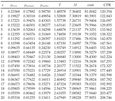
Let us assume that ¼7,m¼1, a¼2,b¼5, am¼m,
andbm¼amþx, for allm1. Forx¼1;2;. . .;20, we show
pover,pnormal,punder,T,M, cost, and CPR for an elastic plat-form in Table 4. It is observed that asxincreases, bothpover and punder decrease significantly, and pnormal (i.e., elasticity TABLE 3
Comparison of Elastic and Inelastic Platforms
c pover pnormal punder probability T M cost CPR
elastic platform 1.25 0.18542 0.26410 0.55048 0.44952 1.37467 10.89474 119.842 164.743 1.50 0.13794 0.46373 0.39833 0.60167 1.44754 10.78981 118.688 171.806 1.75 0.10992 0.58292 0.30716 0.69284 1.52815 10.72906 118.020 180.352 2.00 0.08648 0.67675 0.23678 0.76322 1.64230 10.67876 117.466 192.915 2.25 0.07316 0.72918 0.19766 0.80234 1.73454 10.65005 117.151 203.203 2.50 0.06103 0.77702 0.16195 0.83805 1.85590 10.62435 116.868 216.895 2.75 0.05233 0.81112 0.13655 0.86345 1.97080 10.60592 116.665 229.924 3.00 0.04447 0.84061 0.11492 0.88508 2.11404 10.58911 116.480 246.244 inelastic platform 1.25 – – – 0.24109 2.66581 11.00000 121.000 322.563 1.50 – – – 0.33995 2.66581 11.00000 121.000 322.563 1.75 – – – 0.42592 2.66581 11.00000 121.000 322.563 2.00 – – – 0.50070 2.66581 11.00000 121.000 322.563 2.25 – – – 0.54506 2.66581 11.00000 121.000 322.563 2.50 – – – 0.60432 2.66581 11.00000 121.000 322.563 2.75 – – – 0.65586 2.66581 11.00000 121.000 322.563 3.00 – – – 0.70069 2.66581 11.00000 121.000 322.563
E) increases significantly, due to the increased bm.
Conse-quently, the average task response time increases notice-ably, while the average number of VMs and the cost reduce slightly, and the cost-performance ratio increases signifi-cantly. Therefore, the best auto-scaling scheme is the one withx¼1, a surprising result.
7.2 Optimization of Platforms
In addition to S, the service rate m is also an important parameter that a service provider can decide. One should notice that changingmdoes not mean scale-up or scale-down, since m is pre-set and once set, does not change with the current workload. Intuitively, increasing
m reduces T and M. However, the cost might increase due to the increased dynamic energy consumption. Thus, it is an interesting problem to find the optimal m that minimizes CPR.
Let us consider a¼2,b¼5,am¼m, and bm¼2m, for
allm1. For¼7andm¼1:0;1:5;. . .;5:0, we showpover, pnormal,punder,T,M, cost, and CPR for an elastic platform in Table 5. It is observed that as m increases, both T and M reduce significantly, and both cost and CPR decrease and then increase. Hence, there is an optimal choice ofmwhich minimizes CPR.
7.3 Comparison of Service Providers
In this section, we consider the following problem. For a given application environment specified byandm, how to compare two different cloud service providers specified by P ¼ ða;b; SÞ and P0¼ ða0;b0; S0Þ. Our approach is to com-pare the CPRðPÞ and CPRðP0Þ provided by the two cloud computing platforms.
Assume that¼10andm¼1. PlatformP is specified by
a¼2,b¼5,am¼m, andbm¼2m, for allm1. PlatformP0
is specified bya0¼3,b0¼5,a0m¼m, andb0m¼3m, for all
m1. It is clear that PlatformP0is less responsive, but has faster virtual machine start-up rate. For both platforms, we showpover,pnormal,punder,T,M, cost, and CPR in Table 6. It is observed that PlatformP0 has greater elasticity, longer task response time, less VMs, lower cost, and higher cost-perfor-mance ratio. Thus, PlatformPis preferred to PlatformP0.
8
C
ONCLUDINGR
EMARKSWe have emphasized two significant issues in elastic cloud computing, i.e., the need of a quantifiable, measurable, observable, and calculable metric of elasticity and a system-atic approach to modeling, quantifying, analyzing, and pre-dicting elasticity, and the need of an effective way for prediction, comparison, and optimization of performance and cost in an elastic cloud platform. This paper has contrib-uted significantly to address these two pressing issues. We have not only developed analytical model and method to precisely calculate the elasticity value of a cloud platform, but also applied our model and method to predict many important properties of an elastic cloud computing system and to optimize an elastic scaling scheme and a cloud com-puting platform to deliver the best cost-performance ratio.
The main challenge of our CTMC model is lack of closed-form expressions for its major elasticity, perclosed-formance, and cost metrics, e.g., pover,pnormal,punder,T,M, cost, and CPR. This makes analytical study of an elastic cloud computing platform very difficult. Future research efforts should be directed towards this direction.
A
CKNOWLEDGMENTSThe author would like to express his gratitude to four anon-ymous reviewers for their criticism and comments on improving the quality of the manuscript.
R
EFERENCES[1] M. Aazam and E.-N. Huh, “Cloud broker service-oriented resource management model,” Trans. Emerging Telecommun. Technol., vol. 28, no. 2, pp. 1–17, 2017.
[2] M. Aazam, E.-N. Huh, M. St-Hilaire , C.-H. Lung, and I. Lambadaris, “Cloud customer’s historical record based resource pricing,”IEEE Trans. Parallel Distrib. Syst., vol. 27, no. 7, pp. 1929–1940, Jul. 2016. [3] D. Ardagna, G. Casale, M. Ciavotta, J. F. Perez, and W. Wang,
“Quality-of-service in cloud computing: Modeling techniques and their applications,” J. Internet Services Appl., vol. 5, no. 11, pp. 1–17, 2014.
TABLE 4 Optimal Scaling Scheme
x pover pnormal punder T M cost CPR
1 0.23368 0.17882 0.58750 1.48578 7.36402 81.0042 120.354 2 0.19827 0.30318 0.49854 1.52808 7.30819 80.3901 122.843 3 0.17221 0.39476 0.43303 1.57738 7.26731 79.9404 126.097 4 0.15222 0.46501 0.38277 1.63141 7.23605 79.5966 129.855 5 0.13639 0.52063 0.34298 1.68878 7.21137 79.3251 133.962 6 0.12355 0.56576 0.31069 1.74858 7.19138 79.1052 138.322 7 0.11292 0.60311 0.28397 1.81023 7.17486 78.9234 142.870 8 0.10398 0.63454 0.26148 1.87330 7.16097 78.7706 147.561 9 0.09635 0.66135 0.24230 1.93749 7.14912 78.6403 152.365 10 0.08977 0.68449 0.22574 2.00257 7.13890 78.5279 157.258 11 0.08403 0.70467 0.21130 2.06840 7.13000 78.4300 162.224 12 0.07898 0.72242 0.19860 2.13483 7.12216 78.3438 167.251 13 0.07450 0.73816 0.18734 2.20177 7.11522 78.2674 172.327 14 0.07050 0.75221 0.17729 2.26914 7.10901 78.1992 177.445 15 0.06691 0.76482 0.16826 2.33687 7.10344 78.1379 182.598 16 0.06367 0.77622 0.16011 2.40492 7.09840 78.0824 187.782 17 0.06073 0.78656 0.15271 2.47324 7.09383 78.0321 192.992 18 0.05805 0.79599 0.14596 2.54179 7.08965 77.9861 198.225 19 0.05559 0.80462 0.13979 2.61055 7.08582 77.9440 203.477 20 0.05334 0.81255 0.13411 2.67949 7.08228 77.9051 208.746 TABLE 5 Optimal Service Rate
m pover pnormal punder T M cost CPR
1.0 0.09672 0.66179 0.24148 1.75809 7.13653 78.5018 138.0129 1.5 0.12684 0.56279 0.31037 1.27455 4.83683 64.6925 82.4540 2.0 0.15291 0.49222 0.35487 1.03154 3.69250 66.4649 68.5613 2.5 0.17865 0.44112 0.38023 0.87816 3.00810 77.0826 67.6905 3.0 0.20587 0.40288 0.39125 0.76730 2.55354 94.4809 72.4955 3.5 0.23523 0.37308 0.39169 0.68031 2.23095 117.9612 80.2501 4.0 0.26672 0.34887 0.38440 0.60849 1.99165 147.3819 89.6805 4.5 0.30002 0.32842 0.37156 0.54732 1.80863 182.8975 100.1033 5.0 0.33461 0.31054 0.35485 0.49422 1.66560 224.8560 111.1278 TABLE 6 Comparison of Platforms
Platform pover pnormal punder T M cost CPR P 0.09103 0.66913 0.23984 1.73563 10.14662 111.6128 193.7182