Reduction of Secondary Lobes in Joint angle and
Delay Estimation in Angle of Arrival Localization to
Detect MAC Address Spoofing in Wireless networks
Sara Adel
1and Eman Mohammed
21Department of Information Technology, Faculty of computer and information science, Mansoura University, Egypt 2 Department of Information Technology, Faculty of computer and information science, Mansoura University, Egypt
Abstract: in this paper, we solve the problem of secondary obes that are due to noise that comes from constructive and destructive multipath interference that are resulted in received signal strength (RSS) variation over time. This is to develop a very efficient localization algorithm that uses a unique fingerprint of angle of arrivals (AOAs) , in a specified range, with associated time delays (TDs), in the surrounded sparsity design promoting multipath parameter (i.e:RSS). We solve this problem to detect physical identity spoofing of nodes in radio wireless networks, and localize adversaries and jammers of wireless networks. All radio waves are vulnerable to many types of attacks due to the ability to capture them and sniff or eavesdropping on them in the open space. Physical identity spoofing is used to launch many types of attacks against wireless networks like Denial of Service (DOS), Man-In-The-Middle and Session Hijacking and eavesdropping. Eavesdropping is a human-based social engineering attack. Active adversaries are able to jam and eavesdrop simultaneously, while passive adversaries can only eavesdrop on passed signals. In TCP/IP protocol for example, Media Access Card (MAC) Address is transferred in 802.11 frames. Detection process was carried out by analyzing electromagnetic radio waves that are used to transfer data, in the form of radio wave signals that are formed by the modulation process which mixes the electromagnetic wave, with another one of different frequency or amplitude to produce the signal with a specified pattern of frequency and amplitude. We depended on the angle of arrival of vectors and time delay across scattered areas in the surrounded space to solve the problem of co-location in detection and localization of jammers. We used Maximum Likelihood (ML) angle of arrival determination because Maximum Likelihood approaches, known to their higher accuracy and enhanced resolution capabilities. And we assessed their computational complexity that was considered as the major drawback for designers to their implementation in practice. Our solution was tested on a jammer that changed the signal strength of received signal at the receiver at an angle of arrival 30 degree. And we used scatterers density to determine the angle of arrival of the sender. The simulation has observed that the power of the received signal has changed from the range of angles 20 to 40 degrees. We used scatterers because they describe the density of the signal power, and also enhance the signal to noise ratio, that resulted from the multipath fading of the signal strength. And also overcoming the problem of secondary lobes that are due to signal propagation, while determining the angle of arrival of a signal sender. So, we developed a new passive technique to detect MAC address spoofing based on angle of arrival localization. And assessed the computation complexity of the localization technique through depending on a range angle to estimate the angle of arrival of the adversary within it. And we reduced number of secondary lobes, and their peaks, in the importance function, while determining the angle of arrival, and so increasing the accuracy of angle of arrival measurement. We compared our work to other techniques and find that our technique is better than these techniques.
Keywords: Physical identity address spoofing detection, radio waves, wireless networks, data signal formation and pattern, power delay spectrum and beam width
1.
Introduction
The media access control (MAC) address identifies wireless devices in wireless networks, so it can be used in identity-based attacks. MAC address spoofing is an attack that changes the MAC address of a wireless device that is in a specific wireless network, using off-the-shelf equipment. An attacker can spoof the MAC address of an access point (AP) in WLAN-infrastructure mode and replace or coexist with that AP to eavesdrop or make jamming on the wireless traffic or act as a man-in-the-middle. Also the attacker can flood the network with numerous requests using random MAC addresses to exhaust the network resources. Many methods and researches have been proposed to detect the problem of MAC address spoofing, as in [1] and [2]. In [1] they detected the spoofing attack and localize the adversary. From [3], there are two main types of device localization. The first type is Model-based localization, in which a reference propagation model is used, and localization is depending on received power at a reference distance d0 from the transmitter. And the second type is Fingerprint-based localization, in which the problem of localization is tackled as a classification problem, where each location corresponds to a different class. Our new solution to detection problem depended on solving the problem of co-location in Fingerprint-based localization, such that increasing the accuracy of detection and localization, by means of vectors of angle of arrival of signal components that are local scatterings that occur in proximity to
T
R
x
x
/
antenna [4],and spatial consistency [5]. Spatial consistency is obtained by environment pattern that contains the most effective geometry information. So this environment pattern is useful for generating integral and accurate channel geometry. In MAC address spoofing, spoofed frames are sent out, by the adversary’s rogue device, with spoofed media access card address, resulting in congestion in the network from the quality of service (QOS) and throughput point of view as in [6] and [7], and change in the signal pattern of original legal signal in the physical medium [1]. But for the adversary to know the legal physical identity and spoof it, he firstly must passively sniff on the traffic passing in the propagated signal that is broadcasted in the open and diverse wireless medium space, between a transmitting source of modulated electromagnetic wave, and the destination [6]. And as discussed before, in passive sniffing, the adversary only can eavesdrop on transmitted data, but in active sniffing, the adversary can eavesdrop and jam simultaneously.
by this antenna. The pattern is essentially formed from the radiation characteristics of the antenna itself. Signal strength of a frame means the power level at which this frame can be received at the destination (antenna). We can use this signal pattern to detect and localize the adversary because MAC address spoofing is resulted in many attacks like ARP-DNS-web spoofing- Email spoofing as in [8].and we can guarantee a full secured system if we ensured the security of it’s physical layer. We found that the best way to detect this problem is analyzing the direction of arrival of signal and its vector pattern. We define some of the common notations that will be adopted in this paper, as in [9] where
{}
.
Tand{}
.
Hdenote the conjugate and Hermitian (i.e. transpose conjugate) operators. And as in [6], the transmitted signal from legitimate transmitter and itscovariance matrix are denoted by
s
Z
andG
s={
H}
s
ZZ
E
respectively, with normalized transmit power constraint for this legitimate transmitter, {Gs: Gs
0
,tr
(Gs)} where
sis the maximum tolerable transmission power for it. And the transmitted signal from the active adversary q to destination and its covariance matrix are denoted byz
1
q , and
G
q1=E
{Z
q1Z
Hq1} respectively, with normalized transmit powerconstraint for this
adversary,
{
G
G
G
P
q}
1 q 1
q 1
q
:
≥
0
,
tr
(
≤
, where
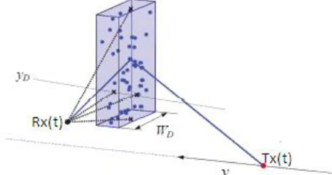
qis themaximum tolerable transmission power for it. In [4], they discussed that determination of angle of arrival in the form of distribution is not impossible but the limitation of measurement of discreteness of angle is resulting from limited width of receiving antenna beam. So modeling local scatterers in the surrounded area of cube like in [5] is very essential to observe local scatterer distribution, by means of significant scatters. Significant scatterers are scatterers that have power greater than a specified threshold [5]. So if we specify a threshold taken from the surrounded environment, such that this threshold differentiates between the presence of an attack from legal transmission, we would detect the presence of anomalies. And if we specify the surrounded are of the receiver as a cube, its width
w
D is defined by the environmental pattern, as it is the range of significant scattered multipath components along the y-axis of the cube as in figure 1. Y-values can be obtained randomly overw
D using uniform discrete probability density function.Note that in [5], they dealt with the surrounding area of transmitter but here we dealt with the surrounding area of receiver to detect the adversary that launches the attack on the receiver. The position of the scatterer is given as
[
x
y
z
qq
q
,
,
], whereq
=
1
,...,
N
sca andN
sca isdetermined by density
x
Q i.e., the number of scatters per cubic meter, and the cube volume. This cube width in space can be used to accurately selecting the sparsity-promoting design parameter
1 that was discussed in [9]. And so we could reduce secondary lobes while obtaining the angle of arrival of these scatterers that are propagated randomly. Andso estimation of number of paths that are depended mainly on sparsity feature that is inherent to marginal delay,
g
( )
iso that we can get time delay estimates from it as was discussed in [9], when a signal hitting multiple receiving antennae in a homogeneous environment.
Figure 1. Geometrical illustration of the scattered multipath Component
In [9], they tackled the problem of joint angle and delay estimation through multiple reflections of a known signal hitting multiple receiving antennae, and they showed that the localization performance was below 15 cm accuracy,but the computation complexity was the main drawback in implementation of the localization technique. In [3] they showed that a distinctive fingerprint for localization can be defined as the vector of RSSI values, and in [7], the detection process depended on observing the effect of the spoofing attacks on the quality of service (QOS) of the network and data rate of spoofed frames flooding. The challenge was that there is no verification mechanism for the nodes’ physical addresses. When we looked at the signal pattern as an area that is formed from spatial points, the Point is considered to be an arbitrary location within an area, and the Event is the observation of this location. The signal strength variation between different points in a specified area is studied as a Mapped Point Pattern, to make a continuous spatial tracing, such that all relevant events were recorded by means of vectors, and the anomalous events were recognized according to spatial continuity analysis.
An attacker can spoof the MAC address of a legitimate wireless device to hide his/her identity to deny service on a given wireless network [6].
In the IEEE 802.11 standards, it is necessary to exchange the four-way handshake frames before an association takes place between a wireless device and the AP. Once the station is associated with the AP, a hacker can disturb this association by sending a targeted deauthentication/disassociation [7] frame to either disconnect the AP by spoofing the MAC address of the wireless user or disconnect the wireless user by spoofing the MAC address of the AP, or sending frames to all of the wireless users using a broadcast address by spoofing the MAC address of the AP. After sending the frame, the AP or the user who receives the frame is disconnected and has to repeat the entire authentication procedure in order to connect again. The attacker can also send spoofed deauthentication frames repeatedly to prevent the wireless user or the AP from maintaining the connection [8].There are also other attacks, such as jamming.
device and rouge device, using RSS samples. We assume that a receiver legitimate station is not mobile. In the jamming period, we can actively send packets to a legitimate device to show scatterrers in RSS samples to measure the angle of arrival. We can detect the attacker if two different locations are returned for the same MAC address.
There are some limitations in the previous work. Sequence number approaches suffer from some drawbacks: control frames don’t have any sequence number at all, spoofing of control frames is possible. Furthermore, some of the tools used by the hackers provide the capability of eavesdropping and injecting frames that have sequence numbers similar to the frames of the legitimate device. OS fingerprinting techniques have some weaknesses, like that data frame only can be detected by the network layer’s OS fingerprinting. Another weakness is that some of the detection techniques assume that the attacker spoofs the MAC address using Linux-based operating system tools. This assumption could cause some attackers to bypass the intrusion detection system. The attackers can use a capability that the Windows operating system provides to change the MAC address of a given user. Finally, vendor information, capability information and other similar fingerprinting techniques can be easily spoofed using off-the-shelf devices. Reccieved signal strength approaches depended on making localization according to the signal strength that is variated due to propagation in the environment. When the attacker and the victim devices are close to each other, the means/medians of both devices are close to each other, so distinguishing the two devices becomes hard. Furthermore, the distribution of the data from a single device can construct two clusters, so it is hard for the clustering algorithm-based approaches to perform well. The purpose is finding a balancing point at which a smaller set of features that let the system to be capable of accurately detecting the node of interest.
2.
Related Work
2.1 Localization through received signal strength:
A previous work in [2], depended on lognormal distribution `of received signal and matching it to the location through the degree of RSS correlation, according to the central tendency of received signal strength values to the medoids of one of two classes, as the aim was to find out the spatial distance in signal (power strength) space between the presence of a spoofing adversary and ordinary legal wireless signal strength. This is determined according to the spatial correlation in signal power strength between spatial points in space which is called by spatial continuity analysis. The main problem is that this correlation is calculated upon the environmental factors affecting the wireless propagated signal. And the main idea of detection depended on cluster analysis by using Partitioning Around Medoids (PAM) method as it was more robust in the presence of noise and outliers, compared to the popular k-means method. In PAM method, spoofing detection depended on spatial correlation between received signal strength, and measured received signal strength, at landmarks, with known reference locations. The received signal strength was considered as test statistic on the distance between two medoids of two partitioned clusters for each node identity, which are legal class cluster and spoofed class cluster.
2.2 Signal strength interpolation
In [10], they depended on interpolating the signal strength values to produce an estimated surface of signal strength values, by using kriging method that takes some known signal strength values of points spaced by a specified distance. But kriging mainly models the spatial structure of measured points to give the estimated surface, according to the specified distance between these measured points. And in [11] for localization, the method of radio frequency fingerprinting-based localization depended on designing datasets containing features that are selected from the RF signal characteristics, in different locations. To form a location fingerprint database, the problem is that it requires forming a tedious site survey that maps RF signals with the physical environment. This requires quite and accurate feature selection for making accurate fingerprints by the selected features. Then testing the fingerprints of RF signals, at random locations in the surveyed area. The signal data would be input to the localization System that uses a classification algorithm, to see the accuracy of finding the true locations of these random fingerprints. The process of producing a fingerprint database on a radio map requires a user to manually tell the system where they are, so that the system can learn the RF signal pattern at that specific location. This is very tedious and time-consuming. And if few features are used to build the fingerprints, the training time and classification time for the machine learning algorithm can be shorter. This is good for real time classification. But fewer features resulted in the difficulty of finding fingerprints that would be unique enough for the localization process. And so higher classification error would be resulted. So the challenge is finding a balancing point at which a smaller set of features that let the system to be capable of accurately detecting the node of interest. The disadvantage of this method is the probability that two locations may be of similar signal pattern.
2.3 Localization through angle of arrival
As discussed in [9], where the reception angle estimation was through joint angle and delay estimation, the system model was for a transmitted signal modulated over M+1 sub carriers. After undergoing multiple reflections, it impinges on the receiving antennae array from Ǭ different
Angles
(
α
1,
α
2,...,
α
Q)
, with associated time delaysQ max Q
2
1
,
Τ
,...,
Τ
)
⊂
[
0
,
Τ
]
Τ
(
, where
maxcan be as largeas desired. And the channel estimates across all antenna elements at each
m
th sub carrier into a single vector,,
)]
m
(
h
),...,
m
(
h
),
m
(
h
[
=
)
m
(
h
1 2 p T (1))
m
(
w
+
e
γ
)
α
(
a
=
)
m
(
h
j2πmΔfTqq q m
∑
(2)Where
w
(
m
)
=
[
w
1(
m
),
w
2(
m
),...,
w
p(
m
)]
T (3), is the corresponding noise vector, andT j j
m j m
m p m
e
e
e
a
(
)
[
21,, (),
22,(),...,
2 ,()]
(4), is the arrayAnd as discussed in [2], the detection depended on the distance between two main medoids of clusters, taking into consideration the parameters of transmission power levels, and distance between spoofing node and original node, and then classifying the multiple number of adversaries into classes. But the main problem with machine learning classification and previous solutions was co-location in which two or more users are in the same place [3].
2.4 Localization through random forests
In [12], they used random forests to make the localization. But signal attenuation that was because of several factors, such as multi-path fading and obstacles that made the signal oscillate, especially when there is a significant distance between the sender and receiving device, and they depended firstly on building a profile of the legitimate device to develop characteristics of normal behavior, assuming that there is no attacker at the stage of building a profile. And this was the first drawback of this solution. The second drawback was that they depended on the fact that RSS samples at a specific location are similar while the RSS samples at two different locations are distinctive, and this is not achieved in all cases because as said before, in section 2.2, two different locations may be of similar signal pattern. And they depended on a machine learning algorithm that requires high set of features, and so higher time consuming, and as said before in section 2.2 the challenge is finding a balancing point at which a smaller set of features that let the system to be capable of accurately detecting the node of interest.
3.
MAC Address Spoofing Detection by
Localization through Angle of Arrival
Determination by using Scatterers
In [4] they depended on clustering of signal components or parameters to estimate angle of arrival distribution. These parameters are defined on the basis of power delay spectrum (PDS) selected points. And they depended on using multiellipical model of delayed scattering component and von Mises’ power delay profile (PDP) for local scattering components, but we depended in obtaining the angle of arrival to locate the adversary, on modeling scattered multipath components, and this can be achieved by observing the distribution of scatterers and their geometry, and using the transfer function of amplitude of scatterers [5] as follows.
(
)
( )
(
)
q φ j q
, R q , T
Sca 4Πfd d t St,f .e
c =
f , t
H
(5)
Where
d
T,q is the time-invariant distance betweenT
X andthe
q
th
scatterer, and
d
R,q( )
t
is the time-varying distance betweenR
x( )
t
and theq
th
scatterer, and
s
( )
t,
f
refers to the scattering coefficient andφ
t
is the random phase modeled by a uniform distribution over [0, 2π).The amplitude of the transfer function is divided into a distance-dependent part, and a scattering coefficient part. So after subtracting the distance-dependent part, the scattering coefficients are evaluated for individual time Instants. It was found that the PDFs of
s
( )
t,
f
at different times can be modeled well by the Gaussian distribution, by which themean values and standard deviations can be estimated using the nonlinear least squares regression method. So, the PDF of the time-varying scattering coefficient is given as:
( )
(
)
(
( )
( )
)
−
−
=
22
2
,
,
exp
2
1
,
f
s s
s
f
t
f
t
S
f
t
s
(6)
Where
μ
( )
t
,
f
s is the mean value at time
t
for frequencyf
. In [4], they discussed that the problem is that no onegeometric model is best by all criteria and for all environments. Because no definite relationship can explicitly associate the parameters of distributions of azimuth and elevation angle, with different types of propagation environments and the distance between the transmitter (Tx) and the receiver (Rx).
But geometric channel model (GCM) can give the possibility of calculating the impact of changes in the position of the objects (TX, Rx), on the spatial properties of the received signals due to the propagation environment type. And the parameters of the GCMs are defined on the basis of the PDS or PDP and the relative position of the transmitter and the receiver. This is because they reproduce the geometry of the spatial relationships among TX, Rx, and the location scattering areas with their spatial density and these criteria differentiate the individual models. And so they provide the basis for theoretical analysis of PDFs of AOA through a statistical model of AOA which is a PDF estimator that is closely related to the type of propagation environment that has temporal characteristics of transmission channel.
4.
Determining Angle of Arrival through
Receiving
Antenna
Beam
Width
to
overcome Co-location problem
Since the idea is that we can detect the Mac address spoofing through the signal strength of frames emitted from a specified node’s Network Interface Card (NIC), then we have looked at the antenna pattern as a group of vectors representing the signal strength and frequency, and the direction of the field received from an antenna. But due to the broadcast nature of signals in wireless medium, and the attenuation that comes out from obstacles that face the signal in the broadcasting medium, the power and direction can be varied. The signal can be exposed to diffraction, scattering, reflection, transmission, and refraction while propagation [13], but because each sending device has it's signal and due to the propagation pattern which can be considered as a fingerprint relating the signal at scattered regions surrounding the receiving node , spoofing detection can be possible if a gap difference in received signal strength of frames with the same Mac address exceeds a specified threshold determined from the spatial continuity analysis and correlation structure of signal propagation in the physical environment in which the signal is broadcasted. We have used Beam forming as in [14], [15] and [16] and the concept of vectors in [9] to determine the directionality of' a signal and so sensitivity from it’s radiation pattern.
discussed in [4] about local and delayed scatterers and that their locations, that we can determine from them, the position of
andR
which are located at a distanceD
So we have showed directional gain antennas when receiving a stream of spoofed frames, the radiation pattern that changed the pattern of the legal sending node, over time to detect the presence of the adversary as well as localizing it. In [9], estimation of number of paths depended mainly on sparsity feature that is related to marginal delay,
g
( )
i that we can get time delay estimates from it. So by accurately selecting the sparsity- promoting design parameter
1, as in [9], and depending on scatterers density and that is also mainly related to path loss characterization in [17] and signal strength attenuation as in [12], we could depend on local scatterers, without depending on signal strength interpolation, so we could reduce the secondary lobes that are due to noise contribution and so reducing the mean square error in equation (5) and (6). Because the role of this design parameter is controlling the spans of main lobes that appear around the true unknown angle of arrivals and time delays. And the parameter
0, that it should be sufficiently high value that is optimized offline according to observed behavior of estimator, as discussed in [9]. We depended on scatterers that defined directionality and gain to make the detection and localization more accurate, in the surrounded scattering areas as in [9], and showed how the distance between transmitter and receiver affected the amplitude of the signal as discussed in [9] and [5]. And so we showed results with the concept of pointing and beamwidth. And we have introduced representative sampling in [18], instead of random windowing, on multiple trace files, to improve coherence discovery in cross spectral density in [19], so that forming links and paths by the number of sampled units taken from the coherent subset. The size of the coherent subset, and inclusion probability that gives the sample size and Depending on the distance function that can calculate the distance between population units in general auxiliary spaces to capture the pattern characteristics. And in [15], the beam is formed at any time n, as y (n) which is a linear combination of the data from M antennas, with x (n) being the input vector and w (n) is the weight vector.)
(
*
)
(
)
(
n
w
n
x
n
Y
=
H (7),Where weight vector
W
(
n
)
can be defined as:
− ==
1 0)
(
M nwn
n
w
(8)And input vector
x
(
n
)
can be defined as
− ==
1 0)
(
M nXn
n
x
(9)In [9], it was discussed that the approximate concentrated likelihood function (CLF) decomposition which is the superposition of the separate contributions pertaining to the
Q
delay pairs, to be separable in terms of the angle-delay pairs as originally required.We can use the equation of PDF of time varying scattering coefficient, (equation (6)), instead of the part of the periodogram of the signal that was discussed in the CLF equation that was equation (38) in [9], as follows:
(
)
=+
Q q q qc
P
M
I
1
,
)
1
(
1
(10)Where
(
)
q q
I
,
is the periodogram of the signal given by:( )
,
=
I
( ) ( )2 1 2 / 2 / ,
2 * 2
= =− − − P p M M m m m p je
h
e
wm j p (11)
In which (m) is the
p
th
element of the vector h (m) And the factor
)
1
(
1
+
M
P
is absorbed in the new designparameter,
p
p
0
1
.And after exploiting the approximation of the above CLF as
importance function (upon normalization) which is equation (40) in [9] as:
( )
(
)
(
)
=
= =
d
d
p
p
Q q q q Q q q qI
I
' ' 1 ' ' 1 1 1,
exp
...
,
exp
,
(12)And after factorizing it in equation (41) in [9], to be separable in terms of the angle-delay pairs as originally required as follows
( )
==
Q q 1,
ḡ
,
(
q,
q)
(13)So, we could carefully design the importance function, and compute time delays and angles of arrival expectations at any desired degree of accuracy, by increasing number of realizations using the corresponding sample mean estimates, as it would be discussed, but in a defined range of angles, where,
ḡ
( )
( )
=
e
e
d
d
I p I p
'
,
,
' ' ' ' , 1 , 1 (14)Is a common private distribution for all angle-delay pairs. So vector realizations
(r)and
(r) can be generated using the multidimensional distribution
( )
,
by generatingQindependent couples
(
r)
q r
q, using ḡ
,
( )
,
thenconstructing
( )
( )
( )
( )
]
,...
,
[
21
r Q r r r=
and( )
( )
( )
( )
]
,...
,
[
1
2
rQ r
r r
=
, by factorizing the jointdistribution ḡ
,
( )
,
as the product of marginal and conditional pdfs, in two equivalent forms, as equations (49) and (50) in [9] as follows:Where ḡ [resp., ḡ
( )
] is the marginal pdf of
[resp.
] and ḡ |(
|
)
[resp., ḡ|(
|
)
] is the conditional pdf of
given
[resp.,
given
]Then we can generate the required realizations through the following two alternatives:
1) Alternative 1: generating
( )rq using ḡ
( )
and thenusing ḡ
(
( )r)
q
=
|
| to generate
( )
r q2) Alternative 2: generating
( )rq using ḡ
( )
and thenuse ḡ
(
( )r)
q
=
|
| to generate
( )
r qBut we selected the first alternative as it was discussed in [9], that the second alternative would be not good option since ḡ
( )
can't allow resolution of closely-spaced angles. And ḡ( )
is able to resolve closely-spaced delays even if the two paths are also extremely closely spaced in the angular domain and it always exhibitsQ
main lobes around the true unknown time delays (TDs),
q
Q
q=1
, and after evaluating ḡ
( )
as equation (51)in [9],as follows:ḡ
( )
=
ḡ,( )
,
d
(17)This is then used to generate
r
thvector of delayrealizations
( )
( )
( )
( )
[
,
,...
]
2 1
r
Q r
r r
=
, then each
q
th
Q
q=1
conditional angle pdf in equation (52) in [9] as: ḡ
(
=
( )r)
=
q
|
, ḡ
( )
(
)
r q
,
, / ḡ
( )
( )
r
q (18),
that is found to exhibit exactly a single main lobe around the true angle
q associated to
q . ḡ( )
was used withlemma 1 to generate required delay realizations
(
)
1
r
q
R
r=
⁓ ḡ
( )
for every q=1,2,3…..,Q
as follows:lemma1: let x
X be any RV with pdff
X(
x
)
and CDF)
(
x
F
X and denote the inverse CDFF
X−1(.)
: [0, 1] →X,u→X such that
F
( )
x
u
X
=
, Then, for any uniform RV,( )
U
X
~
=
F
x−1 is distributed according tof
( )
.
x .
1- Generate R realizations
u
r
q
R
r
)
(
1
= ⁓ U[0,1],
2- Obtain
( )rq =
( )
) (
1 r
q
u
G
− whereG
(.)
is the cumulative distribution function associated to ḡ( )
.The two steps were performed because depending on the SNR, the direct use of the marginal pdf ḡ
( )
faces the following major problems in practice:1-At low SNR, outliers
=G
−1( )
u
, which are delay realizations that don’t correspond to any of the true delays, would appear from realization,u
⁓ U[0,1]that falls within the range of spurious slopes (along the y−axis) in the CDF( )
G
, as seen in Fig. 2(a),Figure 2. Pseudo-pdfs in a single-carrier system illustrated for Q = 2 and SNR = −5 dB: (a) marginal CDF of τ, (b) marginal pdf of τ, (c) local pdf of τ around1, (d) local pdf of τ around
2, (e) local CDF of τ around
1, and (f) local CDF of τ around
2.And which are coming from secondary slopes that are exhibited from ḡ
( )
, as shown in fig. 2(b)This phenomenon is also illustrated in Fig. 2(a) for the two typical realizations
u
andu
. In order to obtain outliers-free realizations, we could rid ḡ( )
from its secondary lobes by choosing a sufficiently large value for the design parameter ρ1. But taking a large value for ρ1, however, renders the main lobes in ḡ( )
extremely narrow making it more likely that the true delays lie outside their very short spans. And so, all outliers-free realizations will be shifted, resulting in an inevitable estimation bias.2-At sufficiently high SNR levels, the secondary lobes are naturally absent and thus a small value for ρ1 can be chosen. Since the difference in main lobes’ sizes results in out-of-proportion slopes in the CDF, an unbalanced number of realizations will be generated under the different main lobes. As a brute-force remedy, one could be tempted by choosing an
To do so, initial estimates of the unknown true TDs, are extracted through broad line search in equation (53) in [9] as follows:
( ) ( ) ( )
,
,...,
Q]
arg
max
Q[
0 02 0
1
ˆ
ˆ
=
( )
(18)Where
arg
max
Q
.
returns the positions of theQ
largest peaks of any objective function. This initial broad line search is performed using a relatively large grid step ∆ , and it doesn’t provide the delay MLEs even by taking an arbitrarily small value for ∆ , because the main lobes of ḡ
( )
are shifted as in figure(3):Figure3. main lobes shifting
And initial estimates for the associated AoAs are obtained as in equation (54) in [9] as:
( )
ˆ
0 =argmaxq
( )
(
ˆ
0)
q= , q = 1 ,…, Q (19) That is performed also with a large grid step. So to force
( )
r qR r=1
and
( )
rq
R r=1
to be generated in the vicinity of
qand
q, respectively, the following Qlocal intervalswere fixed as in [9] as follows:
( ) ( ) ( )
D
q q q − +
=
ˆ ˆ ˆ 0 0 0 , And ( ) ( ) ( )
D
q q q
− +
=
ˆ
ˆ
ˆ
0 0
0
,
Which are centered at
ˆ
( )0q
and
ˆ
( )0q
. And the sizes of local delay and angle intervals are governed by the design parameters
and
, and the associated delay and angle impulse functions were defined as follows:( )
( )
( )
=
otherwise
D
for
h
h
q q q,
0
ˆ
,
ˆ
0 0
(20) ( )( )
( )
=
otherwise
D
for
h
h
q q q,
0
ˆ
,
ˆ
0 0
(21)Then the
q
th delay and angle pseudo-pdfs which are referred to hereafter as local pseudo-pdfs will be used to generate the realizations inD
( )q
ˆ0 andD
( )q
ˆ
0 aregiven by equations (57) and (58) in [9]: ḡ,q
(
)
=
h
q( )
ḡ(
)
(22)ḡ,q
(
)
=
h
q( )
ḡ(
)
(23)For
q
=
1
,
2
,...
Q
, the constantsh
qandh
q, are computed such that the local pseudo-pdfs in (22) and (23) sum up to one thereby yielding equations (59) and (60) in [9] as follows:( ) ( )
( )
1 0 0ˆ
ˆ
−
−
+
=
dt
q q q
h
(24) ( ) ( )( )
1 0 0ˆ
ˆ
−
−
+
=
d
q q qh
(25)Then by applying the impulse functions in (22) and (23), we can obtain a separate isolated local angle/delay pseudo-pdf for each
q
thpath. So, in practice, the processes of generating the required realizations locally around each true delay/angle couple,(
q,
q)
, can be implemented separately and run in parallel with faster and less complex execution. For better illustration, figures 2( c ) and 2(d) show the isolated local delay pseudo-pdfs,
,1( )
and
,2( )
, in case ofQ
=
2
. And as seen from figures 2-e and 2-f, the associated local CDFs,G
,1( )
andG
,2( )
, exhibit a single slope that is located around the corresponding true delay. So by applying the result of lemma 1, each uniform realizationu
q( )r
[
0
,
1
]
will yield a delay realization ( ) ˆ( )0q
D
r
q
in the vicinityof
q. And so all angle realizations that are generated using theq
thisolated conditional pdfs fall in the vicinity of
q. Then we can apply implementation details in section 8 in [9], on equation (6) in this paper, to localize the adversary. These implementation details are:1-Local generation of the required realizations: Step1:
Evaluate the joint pdf
,(
,
)
locally at new discretepoints ( ) ( )
ˆ
ˆ
,
0 0q q
D
D
j
i
as in equation (61) in [9]which is:
(
)
(
)
=
i j broad broad j i j i j iI
p
I
p
,
1
exp
,
1
exp
)
,
(
, (26),
which is the evaluation of the periodogram
I
(
i,
j)
at multiple grid points(
i,
j)
with large discretization stepsbroad
and
broad , and then approximating integrals with discrete sums to evaluate the joint pdfStep2: compute the
q
thmarginal delay pdf at every point( )
ˆ
0 qD
j
as in equation (62) in [9] which is:( )
(
,
)
broad,
i
j i
j
Where the initial delay estimates
ˆ
( )
0
1
q
Q
q=
are the discrete delay points that correspond to the largest
Q
maxima of (27), then for each q=1, 2…Q
, the conditional pdf of theq
thangle corresponding to
ˆ
( )0
q , can be obtained as in
equation (63) in [9] as:
( )
(
=
)
=
(
( )
( )( ))
,
−
2
,
2
,
ˆ
ˆ
ˆ
0 0 , 0 i q q i q i
(27) Then we could have equation (64) in [9] as:( )
=
(
)
small j i j q
,,
( )
ˆ
0 qD
j
(28)Step 3:
Compute the
q
thlocal delay CDF as equation (65) in [9] as follows: small l j l q j qG
=
)
(
)
(
, , ( )
ˆ
0 qD
j
(29)Step 4:
Generate R realizations
( ) Rr r q
u
1
= ⁓
U
0
,
1
and invert(.)
,q
G
via linear interpolation in order to obtain the local delay realizations q( )rG
,q1( )
u
q( )r−
=
for r=1, 2…R.Step 5:
For r=1, 2… R, obtain immediately the local pdf of the
th
q
AOA conditioned on
q( )r from the local joint pdf that are evaluated in step1 as equation (65) in [9] as follows:( )
(
)
(
( )
( )( ))
r q q r q i r q i , ,
,
=
=
( )
ˆ
0 qD
i
(30)Step 6:
Evaluate the
q
thlocal angle CDF,( )
iq
G
,
similarly to,( )
j qG
,
, in (29), and generate ther
th angle realization
q( )r=
G
−,1q( )
u
q( )r , using linear interpolation also.2-Estimation of time delays and angle of arrivals
After generation of all the required realizations, more accurate IS-based parameter estimates can were obtained by applying the circular sample mean instead of the linear sample mean. Because the latter averages out all the realizations and outlier seeds will result in an inevitable estimation bias. However, the circular mean succeeds in selecting the best angle and delay realizations in terms of Euclidean distance to the true multipath-resolution parameters. The circular mean of any transformation
f
( )
of a given random variable
−
[
, ]
with distribution( )
p
is obtained as equation (66) in [9] as follows:( ) ( ) 1
1
ˆ
R(
r)
j rr
f
e
R
==
(31)Where, where φ(r) ∼ pΦ(.) are R realizations of Φ.
We need to transform
q( )r and
q( )r that are respectively inmax
[0,
]
and[
−
/ 2,
/ 2]
into interval[
−
, ]
.So transformations( ) ( )
1
(
)
2 (
/
max1/ 2) [
, ]
r r
q q
=
−
−
and( ) ( )
2
(
)
2
[
, ]
r r
q q
=
−
, were applied for UniformLinear Arrays (ULAs ).so the circular mean is first applied using
1(
q( )r)
and( )
2
(
)
r q
, then the true TDs and AoAs are then estimated using the inverse transformations1
1 max
1
1
( )
(
)
2
2
x
x
−
=
+
and 21( )
1
2
x
x
−
=
as as in equations (67) and (68) in [9] as follows:( ) ( )
(
)
( )
+
=
= −2
1
,
2
1
ˆ
1 2 1 2 max max R r j r r q r qe
(32) ( ) ( )(
)
(
( ))
=
= − R r j r r q r qe
1 2,
2
1
ˆ
(33)Where the weighting coefficient was expressed as equation (69) as:
( ) ( )
( ) ( ) 0
( ) ( )
1 1
exp{
(
,
)}
(
,
)
exp{
(
,
)}
r r
r r c
Q r r
q q q
P
P
I
==
(34)where
1 1
0
... exp{
(
,
)}
... exp{
( , )}
Q
q q q
c
P
I
d d
P
d d
=
=
(35)By defining the quantity:
Ψ
( , )
0 11
( , )
(
,
)
Q
c q q
q
P
P
I
=
−
(36)And using the following normalized weighting coefficient
( ) ( )
(
r,
r)
exp
=
{Ψ ( ) ( )(
r,
r)
-1
max
r R
Ψ
( ) ( )
(
r,
r)
} (37)instead of the weighting coefficient in (34) To reduce the computational load with no changes in the final results.
To generate vector realizations that jointly minimize the Euclidean distance to the true delay and angle parameters, such that: ( ) ( ) 2 2 ( ) ( ) ,
ˆ
ˆ
[ , ]
arg min(
)
r r
r r
=
−
+
−
(38)This is according to lemma 2 which says that:
The circular-mean estimates
1 2
ˆ
[ ,
ˆ ˆ
,...,
ˆ
]
Q