Vol 4 (2015)

Regression Analysis of the Left–ventricular

Isochoric Pressure Decay of the Heart:

Four or Five Model Parameters?

Stefan F. J. Langer

Institute of Physiology, Charité University Medicine, Berlin, Germany.

Introduction

Biophysical models predicting the relaxation of cardiomyocytes1 take into account a lot more variables than regression models analysing the left ventricular relaxation in human and animal hearts. These isochoric (isovolumic) pressure decay curves are often described by an exponential2 _{or logistic}3 _{time constant.} Both these three–parametric regression models are regarded unsatisfactory4, 5_{. Consequently, a four–parametric extension of} the logistic (or: hyperbolic tangent) model was introduced4_,

(1)

(Langer model), estimating initial, P₀, and asymptotic, P_∞, pressure, asymptotic time constant,τ_τ∞, and a shape factor, γ. This model encompasses both the exponential (by γ = 0) and the logistic (_{γ = 0.5) model, and it yields fairly normally} distributed regression residua6_.

A recent series of articles7, 8, 9 _{proposes a five–parametric model} according to the well known differential equation of a damped oscillation,

(2)

to describe the isochoric pressure decay (kinematic Chung model). This results in three types of pressure decays,

where (Eq. 2A) holds if _β2 _{< E, undercritical damping, (Eq. 2B)} if _β2 _{= E, critical damping, and (Eq. 2C) if β}2 _{> E, overcritical} damping. We unify the parameters by introducing the initial pressure change velocity, P₀, and obtain in the respective case:

Abstract

Background

Isochoric (isovolumic) cardiac pressure decay data were previously described by a four–parametric logistic (tangens hyperbolicus) regression model (Langer model). However, a five–parametric kinematic model (Chung model), according to the differential equation of damped oscillation, was recently introduced to describe the isochoric pressure fall. The present study clarifies (a) whether these five parameters can be reliably estimated from empirical pressure decay data and if the model excels the four– parametric one, and (b) whether the kinematic Chung model validly describes these pressure decays.

Methods

High–fidelity intraventricular pressure decay data from 1203 isolated working guinea pig and rat hearts were analysed by both models. Results

Most cases present with a higher regression error in the five–parametric kinematic model, the median ratio (F value) of its regression variance by those of the four–parametric logistic model is 1.056 (95 per cent confidence interval: 1.037 to 1.084) in the guinea pig and 1.040 (1.027 to 1.061) in the rat group. Additionally, the parameters of both models were estimated from the first and second half of the decay phase separately to check for the models’ validity. The five– parametric model yields significantly non–constant parameters more often than the four–parametric model.

Conclusion

(a) The five parameters of the kinematic Chung model remain underdetermined by the empirical pressure data, and (b) this five– parametric model does not provide a valid description of the isochoric cardiac pressure decay.

Key words: ventricular pressure; diastole; relaxation; regression analysis; hemodynamics

Citation: Langer, S.F.J. Regression Analysis of the Left-ventricular Isochoric Pressure Decay of the Heart: Four or Five Model Parameters? International Cardiovascular Forum Journal. 2015;4:53-58 DOI: 10.17987/icfj.v4i0.168

ISSN: 2410-2636 © Barcaray Publishing * Corresponding author. E-mail: [email protected]

However, the achievement of the four–parametric model4, 6_{, Eq.} 1, renders the reliability of estimating fiveparameters from the

juxtaposed with three-parametric models7, 8_{; a comparison} to four–parametric alternatives is lacking. Furthermore, the model supposes constant parameters in describing a concrete pressure course; this is a doubtful assumption8_{. Therefore, the} present statistical analysis aims to clarify: (a) Does the five -parametric Chung model improve the goodness–of–fit

significantly, compared with the four–parametric Langer model? This includes the reliability of estimating fiveparameters from the pressure data. (b) Do the model parameters remain constant during the pressure decay, as demanded by the respective differential law?

Methods

Preparation and numerical regression methods are previously described in detail4_.

Preparation

In short, hearts of male Sprague–Dawley rats and mixed–breed guinea pigs of both sexes were mounted to an artificial working heart circulation, perfused with O₂ saturated bicarbonate buffer, 37˚C, 2.5 mM Ca2+_{. After steady–state settled at cardiac output} about 40 mLmin−1 _{and mean aortic pressure of 80 mmHg} (rats) or 60 mmHg (guinea pigs), one left–ventricular pressure curve (length 4 seconds, digitized at 1 kHz) was obtaind from each specimen by an intracaval subminiatur manometer. The isochoric pressure decay phases (beginning at maximum pressure fall velocity, ending at the reencounted end–diastolic pressure) were automatically extracted from each interval and pooled by adjusting the time axis for a minimal standard deviation. Intervals were discarded for lacking eurythmicity or poor steady–state if the standard deviation within the pooled consecutive decay phases exceeded 0.50 mmHg in guinea pig or, according to their higher aortic pressure, 0.63 mmHg in

rat hearts. This criterion removed less than 5 per cent of each species sample. Samples with duration of the isochoric phase data questionable. The five-parametric regression was solely being too short for a halfwise regression (see below, Statistics b) were disregarded in this particular analysis. The Tables give absolute numbers.

All animals recieved human care according to the Tierschutzgesetz (German Animal Protection Act). Each specimen was subsequently utilised in other research not presently mentioned.

Statistics

Regression fits were calculated by the downhill simplex method10_{. To protect against spurious numerical error minima,} each analysis was repeated with 8r sets of initial guesses by allotting 8 different initial values to each of the r model parameters2_{. Each sample underwent two analyses:}

(a) Chung and Langer model were fitted to the pressure decay data, see Fig. 1, right. Median standard error of regression and its 95% interval of confidence are presented for both species. The regression variances of the Chung model were divided by those of the Langer model, the resulting F values compared against the F–distribution (single–sided Fisher test); significant advantage of the five–parametric Chung model is assumed at p < 0.05.

(b) For comparing parameters estimated from the first and second half of the individual pressure decay phase, the latter was previously corrected by subtracting a damped oscillation (third heart sound) term which was obtained by regression analyses of the residua left by the two models, as mentioned above. Again, Chung and Langer model were applied to the corrected data and, subsequently, to the first and the second half of the pressure decay phase seperately. Significantly non– constant model parameters were assumed if the halfwise

Figure 1: Isochoric left–ventricular pressure (LVP) decay with fitted

regression models. Fourteen consecutive decay phases of an isolated working rat heart.

Gray: regression curves of the 4–parametric Langer model (solid) and the 5–parametric Chung model (dotted). Time– course (right) and derivative– vs.–pressure (“pressure phase plane”) diagram (left,

notice the axes’ directions).

ICFJ — Regression Analysis of the Isochoric Pressure Decay

3

-3000 -2000 -1000 0

LVdP/dt [mmHg/sec]

t [msec]

-3000 -2000 -1000 00 0 10 20 30 40

10 20 30 40 50 60

LVP [mmHg]

Fig. 1.

Isochoric left–ventricular

pressure (

LVP

) decay with fitted

regression models.

Fourteen

consecutive

decay

phases

of

an isolated working rat heart.

Gray

: regression curves of the

4–parametric

Langer

model

(solid)

and

the

5–parametric

Chung model (dotted).

Time–

course (right) and derivative–

vs.

–pressure

(”pressure

phase

plane”) diagram (left, notice the

axes’ directions).

an intracaval subminiatur manometer. The isochoric pressure decay phases (beginning at

maximum pressure fall velocity, ending at the reencounted end–diastolic pressure) were

au-tomatically extracted from each interval and pooled by adjusting the time axis for a minimal

standard deviation. Intervals were discarded for lacking eurythmicity or poor steady–state

if the standard deviation within the pooled consecutive decay phases exceeded 0.50 mmHg

in guinea pig or, according to their higher aortic pressure, 0.63 mmHg in rat hearts. This

criterion removed less than 5 per cent of each species sample. Samples with duration of the

isochoric phase being too short for a halfwise regression (see below, 2.2

b

) were disregarded

in this particular analysis. The Tables give absolute numbers.

All animals recieved human care according to the

Tierschutzgesetz

(German Animal

Pro-tection Act). Each specimen was subsequently utilized in other research not presently

men-tioned.

2.2

Statistics

Regression fits were calculated by the downhill simplex method [10]. To protect against

spurious numerical error minima, each analysis was repeated with 8

_{sets of initial guesses}

by allotting 8 different initial values to each of the

r

model parameters [2]. Each sample

underwent two analyses:

(

a

) Chung and Langer model were fitted to the pressure decay data, see Fig. 1, right.

Median standard error of regression and its 95% interval of confidence are presented for both

species. The regression variances of the Chung model were divided by those of the Langer

model, the resulting

F

values compared against the

F

–distribution (single–sided Fisher test);

significant advantage of the five–parametric Chung model is assumed at

p <

0

.

05.

(

b

) For comparing parameters estimated from the first and second half of the individual

pressure decay phase, the latter was previously corrected by subtracting a damped oscillation

(third heart sound) term which was obtained by regression analyses of the residua left by

the two models, as mentioned above. Again, Chung and Langer model were applied to

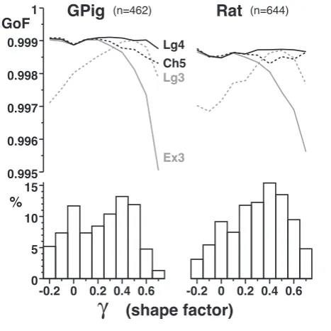
Figure 2: Distribution of shape factor (γ) and goodness–of–fit (GoF)

among isochoric left–ventricular pressure decays of guinea pig and rat hearts. Three–parametric exponential (Ex3) and logistic (Lg3) regression model, 4–parametric Langer (Lg4) and 5–parametric

Chung model (Ch5). Samples from Table 2.

ICFJ — Regression Analysis of the Isochoric Pressure Decay

4

0.995 0.996 0.997 0.998 0.999 1

GPig

GoF

(n=462)

Rat

-0.2 0 0.2 0.4 0.6 0

5 10 15

%

-0.2 0 0.2 0.4 0.6

(shape factor)

γ

Fig. 2.

Distribution of shape

fac-tor (

γ

) and goodness–of–fit (

GoF

)

among isochoric left–ventricular

pressure decays of guinea pig and

rat hearts. Three–parametric

ex-ponential (

Ex3

) and logistic (

Lg3

)

regression model, 4–parametric

Langer (

Lg4

) and 5–parametric

Chung model (

Ch5

).

Samples

from Table 2.

the corrected data and, subsequently, to the first and the second half of the pressure decay

phase seperately. Significantly non–constant model parameters were assumed if the halfwise

regression yields lower residual variance compared to the overall regression, with

p <

0

.

05.

Median relative differences of the halfwise estimated model parameters and the respective

estimates from the full sample are presented with 95% intervals of confidence.

3

Results

Most isochoric pressure decays present with an intermediate shape, between

exponen-tial (

γ

= 0) and logistic (

γ

= 0

.

5) curve, see Fig. 2. As expected, the three–parametric

models fail to fit curves well, if

γ

becomes high or low, respectively. In contrast, the

four–parametric Langer model describes all pressure curves equally well, whereas the

five–parametric Chung model yields inferior goodness–of–fit on curves with

γ >

0

.

2, as

also seen from Fig. 2. Two thirds of of the samples in each species are better fitted by

the four– instead of the five–parametric model, with a median ratio of residual

regres-sion variances (

F

values) significantly in favor of the four–parametric model, see Table

1. Significantly less than ten per cent of the samples allow for a statistically proved

advantage of the Chung model (individual

p <

0

.

05, not adjusted for the multiple

testing). The Chung model predicts overcritical damping (i.e., no inflection point) in

92.2 per cent (89.3–94.5, 95% confidence interval) of the guinea pig and in 80.2 per

cent (76.8–83.2) of the rat hearts.

regression yields lower residual variance compared to the overall regression, with p < 0.05.

Median relative differences of the halfwise estimated model parameters and the respective estimates from the full sample are presented with 95% intervals of confidence.

Results

Most isochoric pressure decays present with an intermediate shape, between exponential (γ = 0) and logistic (γ = 0.5) curve, see Fig. 2. As expected, the three–parametric models fail to fit curves well, if γ becomes high or low, respectively. In contrast, the four–parametric Langer model describes all pressure curves equally well, whereas the five–parametric Chung model yields inferior goodness–of–fit on curves with _{γ > 0.2, as also seen} from Fig. 2. Two thirds of the samples in each species are better fitted by the four– instead of the five–parametric model, with a median ratio of residual regression variances (F values) significantly in favor of the four–parametric model, see Table 1. Significantly less than ten per cent of the samples allow for a statistically proved advantage of the Chung model (individual p < 0.05, not adjusted for the multiple testing). The Chung model predicts overcritical damping (i.e., no inflection point) in 92.2 per cent (89.3–94.5, 95% confidence interval) of the guinea pig and in 80.2 percent (76.8–83.2) of the rat hearts.

Applying the four–parametric Langer model to the first and second half of the pressure decay phases, thus doubling the number of regression parameters, worsened the regression variance in significantly more than half of the samples of each species, see F values in Table 2. In contrast, halfwise regression

with the five–parametric Chung model decreased the regression variance in more than half of the samples (albeit the median F does not significantly differ from one in the rat sample). This difference between the models is significant in both species, and is confirmed by the considerably different numbers of individually significant improvement of fits (p < 0.05 in Table 2).

Furthermore, Table 2 shows the relative aberrances of the initial (at t = 0) pressure and pressure derivative, estimated from the first and second half, respectively, from the estimates obtained by the overall regression. The first–half estimates of these values do not differ considerably from the usual overall regression (both models, both species).

This also holds true for estimating the initial pressure from the second half of the decay phase. However, both models considerably overestimate the initial pressure fall velocity (too negative derivative) from the second half of the decay phases, where the error of the five–parametric model is a manifold of this obtained by the four–parametric one. In the Chung model, even the damping characteristic (under/ overcritical damping) may differ among overall and halfwise regression: 8.2 per cent (5.8–11.2, 95% confidence interval) of the guinea pig samples present with a different characteristic of the first half, and an equal portion presents with a different characteristic of the second half of the decay phase, each compared with the overall curve shape. Among the rat hearts, 17.8 per cent (4.9–21.1) of the first and 19.8 per cent (16.8–23.2) of the second halves differ from the damping type of the whole decay phase.

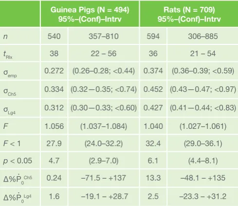
Table 1: Regression errors in left–ventricular pressure decays

Guinea Pigs (N = 494)

95%–(Conf)–Intrv 95%–(Conf)–IntrvRats (N = 709)

n 540 357–810 594 306–885

t_Rlx 38 22 – 56 36 21 – 54

σemp 0.272 (0.26–0.28; <0.44) 0.374 (0.36–0.39; <0.59) σCh5 0.334 (0.32—0.35; <0.74) 0.452 (0.43—0.47; <0.97) σLg4 0.312 (0.30—0.33; <0.60) 0.427 (0.41—0.44; <0.83) F 1.056 (1.037–1.084) 1.040 (1.027–1.061)

F < 1 27.9 (24.0–32.2) 32.4 (29.0–36.1)

p < 0.05 4.7 (2.9–7.0) 6.1 (4.4–8.1)

Δ%P0Ch5 0.24 –71.5 – +137 13.3 –48.1 – +135

Δ%P0Lg4 1.6 –19.1 – +28.7 2.5 –23.3 – +31.2

Values are sample medians or percentages. Number (n) of data points per sample and duration (tRlx, msec) of isochoric pressure decay with central 95% range. Empirical standard deviation (σemp, mmHg) of the overlayed pressure decay data; standard regression errors of the 5–parametric Chung model (σCh5, mmHg) and the 4—parametric Langer model (σLg4, mmHg), with 95% confidence limits of the median and upper 95% confidence limit of the 95%– quantile (<). F = (σCh5/σLg4)2. Percentages of samples better (F < 1) and significantly better (p < 0.05) fitted by the Chung model, with 95% confidence limits. Δ% P0Ch5,Lg4: relative deviation of the initial pressure fall velocity, as estimated by the Chung and Langer model, respectively, from the observed value, with central 95% range.

Table 2: Regression errors of overall and halfwise fits

Guinea Pigs (N = 462) Rats (N = 645)

Ch5 Lg4 Ch5 Lg4

F 0.996 0.9998_0.991 1.004 1.006_1.002 0.998 1.002_0.993 1.004 1.006_1.002

F < 1 55.2 59.8_50.5 40.0 44.7_35.5 *51.5 55.4_47.5 *43.9 47.9_40.0

p <

0.05 12.1 15.5

9.2 2.2 4.0 1.0 16.4

19.6 13.6 5.0

7.0 3.4

Δ%P0(1) _0.012 0.024 0.003 0.089

0.114 0.071 0.024

0.038 0.015 0.183

0.214 0.151

Δ%P0(2) _3.1 3.9 2.0 –0.40

0.39 −1.10 5.6

7.0

4.3 5.2

6.8 3.4

Δ%P0(1) _0.050 1.7 −1.3 –1.7

−1.1 −2.1 –3.1

−0.99 −4.5 –3.5

−2.8 −4.1

Δ%P0(2) _–145 −99

−190 1.1 −2.03.1 –81 −112−42 –17.2 −12−23

Values are sample medians or percentages with upper and lower 95% confidence limits. Ch5, 5–parametric Chung model; Lg4, 4–parametric Langer model. F, ratio of regression variance of the halfwise by that of the overall fit; p, error probability in assuming F < 1 in the individual specimen. Δ%P0(h) , percentage deviation of the initial pressure estimated from the first (h=1) and second (h=2) half of the pressure decay phase from P₀ (overall fit).

Accordingly: Δ%P0(h), initial pressure change velocity, as estimated by Ch5 and calculated from Lg4–parameters, respectively. *:These figures differ significantly (two–sided p < 0.007), in spite of slightly overlapping confidence intervals.

.

.

Discussion

For statistical reasons, the “top down” modeling of a biosignal — ventricular pressure, presently — by regression analysis is restricted to few model parameters. Biophysical ”bottom up” models usually consider much more factors even to describe the behaviour of the myocardial fiber, such as 22 parameters for contraction and relaxation1_{. Transforming this one dimensional} tension to intracaval pressure requires even more (spatio– temporal) parameters among which the anatomical orientation of the myofibrils takes a significant influence on the pressure relaxation curve11_{. Since these anatomical relationships} are a subject of evolutionary optimization, the shape of the descending ventricular pressure curve may correspond approximately to the myofibrillar relaxation. Despite this simplification, the number of biophysical factors exceeds the number of reliably estimable regression parameters. Present results suggest that regression models may contain no more than four parameters.

Exponential regression with zero12 _{or estimated asymptote}2 _as well as the three–parametric logistic regression3 _{are well known} to fail in modeling the isochoric left–ventricular relaxation, i.e., the pressure decay curve4, 7, 12_{. Extending the logistic model by} a fourth (“shape”) parameter4 _{yields a model (Eq. 1) that fits} equally well to exponential, logistic, and intermediate curves; its regression residua were found to be normally distributed in isolated working small animal hearts after correcting for an acustomechanical disturbance6_{. More recently, Chung et al.}7 introduced a five–parametric “kinematic” regression model (Eq. 2A–C). This model was subsequently used to obtain a load–independent lusitropic index8 _{and to cover spatio–} temporal variation of camber relaxation9_{. It provides a better} fit to a wider range of pressure, pressure derivative, and phase plane curves than the three–parametric models7, 8, 9 _{and was} claimed to be physics– and physiology–based7_{. However, the} five–parametric Chung model was not yet compared with any four–parametric alternative. Claims on no mathematical link between the exponential and logistic time constant7_{, or that} these time constants were previously unrelated9_{, do not hold. A} mathematically contiguous and physically sound link between exponential and logistic time constants has been published and validated4, 6_{. Furthermore, the original study}7 _initially presents three types of curves, well exponential (“linear”), well logistic (“curvilinear”), and intermediate, respectively, but the intermediate data were eventually merged to the “linear” group, thus disadvantaging the exponential model (see Fig. 2). Exponential time constants were obtained by linear fits in the phase plane7_{, thus amplifying measuremental errors, whereas} the regression analysis demands an error–free abscissa.

Regression errors of the four– and five–parametric

model

Pressure curves, as any empirical data, provide limited information; therefore, the number of regression model parameters must not be increased deliberately. Consequently, four–parametric models, not only three–parametric ones, must be ruled out before further increasing the number of parameters. Sound statistics and sufficient sample sizes are necessary to proof for pertinent model differences. The present number of samples allow for calculating meaningful confidence intervals for the medians. Pairwise tests on significance are unnecessary because non–overlapping confidence intervals prove for a significant difference (p < 0.05) in the present study; only in (one, Table 2) case of slightly overlapping confidence intervals, the two–sided p value was calculated.

The first investigation, Table 1, found significantly better fits of the four–parametric Langer model, and a percentage of individually significant advantage of the five–parametric Chung model only in the range of the error probability (5%). Such ad- vantage is just by chance. Due to the sample sizes, the failure of the Chung model to enhance the regression must not be attributed to the number of model parameters differing by one. More probably, the inability of the Chung model to describe logistic curve forms is liable, as shown by Fig. 2. Contrary observations on the Chung model fitting “all cases” of pressure decays in a mathematically precise manner8 _{do not hold} in the light of calculus: the differential law (Eq. 2) of the Chung model only covers the exponential case but does not comply with the differential law of a logistic curve4_{. Another explanation} may be provided by the quite normally distributed residua already leaved by the four–parametric regression6_{: in such} cases, a model with more parameters may be underdetermined by the measured data, i.e., considerably different sets of parameters may fit equally well to the data.

This was exemplarily checked by comparing the model predicted initial pressure decay velocity with the observed (maximal negative) slope of the pressure curve (Table 1). Both models present with a considerable scattering range which may be explained by the well–known error amplifying effect of differentiation. However, that scattering is more than double as broad in the Chung model, almost rendering the estimated values meaningless. This result conflicts with previously reported good agreement between empirical and Chung–predicted maximal pressure fall velocitiy7_{. However,} that pressure curves were digitized at only 200 Hz, heavily smoothed by a gliding 20 millisecond averaging window and transformed into the derivative–vs.–pressure phase plane, thus feeding error–amplyfied derivative data to the model. Such data transforming and smoothing is deprecated because the regression process already performs the desired kind of averaging and must be the exclusive source of such averaging, if reliable results are expected.

Model validation by halfwise regression fits

The second part of the present study checked for the validity of the models decribing the isochoric pressure decay. Validity is assumed if a model fits the data with no systematic error. Consequently, the parameters estimated from a subset of a sample must resemble those estimated from the whole sample. However, the isochoric pressure decay is distorted by an acustic oscillation, triggered by the aortic valve closing, that depresses early and augments later pressure values6_. This oscillation was removed from the samples to facilitate the halfwise regressions for that reason; such filtering is unnecessary while using the whole isochoric phase6_{, as in the} first part of the present analysis.

In Table 2, F < 1 indicates violation of the respective model by the individual sample, because in these cases the sum of regression variances of the two halfwise fits becomes smaller than the variance of the overall fit to the sample. Contrary, F

isochoric pressure fall can be expected from the Chung model. In contrast, the respective results do not raise any objection against the four–parametric logistic model.

Physiological model interpretations

Time constants are commonly called for being purely empirical indexes7, 12_{, just because no formula is known to calculate} the pressure decay curve in terms of ventricular anatomy and myocytal biophysics. It should be stressed that the exponential time constant indeed has a well known physical meaning as being the quotient of viscosity (resistive term) by elasticity13_. Correlation between this time constant and the respective quotient, 2_{β/E, of Chung–parameters}7 _{is not a surprise,} therefore. The three–parametric models do not allow to

seperate viscous (nominator) and elastic (denominator) terms. In contrast, model (Eq. 1) provides two time constants, the initial τ0 = τ∞/(1 − γ) and the asymptotic τ∞ itself. Further research may introduce physiologically reasonable assumptions that allow to separate viscous and elastic term from this additional information.

However, albeit claimed9_{, and in contrast to what (Eq. 2) may} suggest, the Chung model does not separate these terms, just because it implies constancy of both, which is not the case. Otherwise, their quotient, i.e., the “local” time constant, must be also constant, but the four–parametric logistic model already reveals a decreasing time constant during most pressure decays. The mere existence of inertia, elasticity, and friction does not imply constancy and does not render (Eq. 2) becoming model–based in a physical sense; an averaging or “lumping” is not allowed in the time domain, because non–constant parameters disqualify the equation. Especially the beginning isochoric phase is still influenced by the formerly expelled blood7_{; but afterwards the closed aortic valve prevents that} momentum from swinging back, thus changing the inertia term.

After model (Eq. 2) collapses, because its constants do not remain stationary during the regression period, it leaves (Eqs. 2A–C) becoming just another purely empirical functions that may be used to describe pressure decays. Many elementary and transcendent functions are on hand that fit very neatly to pressure fall curves, if scaled by at least four regression parameters4_{. Accordingly, only the observed curves can decide} which function should be adopted. This requires powerful statistics, because minute differences have to be dealt with. As the present study demonstrates invalidity of the five– parametric model, previous deductions should be revised. For example, an inflection in the pressure fall curve was deduced from the Chung model to occur by physical necessity7_{; however,} this model failed to predict any inflection in more than 80 per cent of the present samples. In contrast, the Langer model, as based on the hyperbolic tangent function, always predicts existing inflection points and also correctly indicates the non– inflecting (i.e., exponential) curves.

Limitations

The present study is restricted to freshly isolated, small animal hearts of two species under specific standard working condition. Concerning the species restriction, pressure decay curves of rat and guinea pig ventricles do not remarkably differ from those in canine3_{, human}12, _{or mouse}5 _{hearts. Depressed} hearts are reported to present with curve shapes different from those seen in well performing ventricles5, 14_{. The presently} studied four–parametric model was previously seen to fit data from broadly varied condition with just a moderate increase of

the standard error range4_.

Conclusion

a) Applying the five–parametric kinematic regression model (Eq. 2) to isochoric cardiac pressure decays is statistically unjustified, because regression fits by the four–parametric logistic model (Eq. 1) yield the smaller residua. b) The isochoric pressure decay does not resemble a damped or (over)critically damped oscillation law. Even in species and conditions presently not investigated, the reliability of relaxation models with more than four parameters should be doubted.

Statement of ethical publishing

The author states that he adheres to the statement of ethical publishing of the the International Cardiovascular Forum Journal15_.

Acknowledgement:

The author thanks the Sonnenfeld Foundation, Berlin, who partly financed the laboratory equipment.

Conflict of interest:

The author is not in conflict concerning interests.

Address for correspondence:

Guineastr. 14, 13351 Berlin, Germany Phone +4930 24615437

E-mail: [email protected]

References

1. Niederer SA, Hunter PJ, Smith NP. A quantitative analysis of cardiac myocyte relaxation: A simulation study. Biophys. J. 2006;90: 1697–1722 (DOI: 10.1529/biophysj.105.069534).

2. Craig WE, Murgo JP. Evaluation of isovolumic relaxation in normal man during rest, exercise and isoproterenol infusion [abstract]. Circulation 1980;62 (Suppl. II): 92.

3. Matsubara H, Araki J, Takaki M, Nakagawa ST, Suga H. Logistic characterization of left ventricular isovolumic pressure–time curve. Jpn. J. Physiol. 1995;45: 535–552 (DOI: 10.2170/jjphysiol.45.535).

4. Langer SF. Differential laws of left ventricular isovolumic pressure fall. Physiol. Res. 2002;51: 1–15 (http://www.biomed.cas.cz/physiolres/ pdf/51/51_1.pdf).

5. Cingolani OH, Kass DA. Pressure–volume relation analysis of mouse ventricular function. Am. J. Physiol. Heart. Circ. Physiol. 2011;301: H2198–H2206 (DOI: 10.1152/ajpheart. 00781.2011).

6. Langer SF. Ransacking the curve of cardiac isovolumic pressure decay by logistic–and–oscillation regression. Jpn. J. Physiol. 2004;54: 347–356 (DOI: 10.2170/jjphysiol.54.347).

7. Chung CS, Kovács SJ. Physical determinants of left ventricular isovolumic pressure decline: model prediction with in vivo validation. Am. J. Physiol. Heart. Circ. Physiol. 2008;294: H1589–H1596 (DOI: 10.1152/ ajpheart.00990.2007).

8. Shmuylovich L, Kovács SJ. Stiffness and relaxation components of the exponential and logistic time constants may be used to derive a load–independent index of isovolumic pressure decay. Am. J. Physiol. Heart. Circ. Physiol. 2008;295: H2551–H2559 (DOI: 10.1152/ ajpheart.00780.2008).

9. Ghosh E, Kovács SJ. Spatio–temporal attributes of left ventricular pressure decay rate during isovolumic relaxation. Am. J. Physiol. Heart. Circ. Physiol. 2012;302: H1094–H1101 (DOI: 10.1152/ ajpheart.00990.2011).

10. Press WH, Flannery BP, Teukolsky SA, Vetterling WT. Numerical Recipes: The Art of Scientific Computing, 3rd ed. Cambridge: Cambridge University Press 2007.

12. Eschmann P, Krayenbühl HP, Rutishauser W. Druckverlauf bei der isovolumetrischen Relaxation des linken Ventrikels des Menschen im Ruhezustand und unter akuter Druckbelastung. Z. Kardiol. 1975;64: 444–460.

13. Bland DR. The Theory of Linear Viscoelasticity. Oxford: Pergamon Press 1960.

14. Langer SF, Schmidt HD. Influence of preload on left ventricular relaxation in isolated ejecting hearts during myocardial depression. Exp. Clin. Cardiol. 2003;8: 83–90 (http://www.ncbi.nlm.nih.gov/pmc/articles/ PMC2716204).