http://scienceasia.asia
_______________
Key words and phrases: Method of Variation of Parameters; Periodic Orbits; Oblateness; Radiation Pressure; The Restricted Three-Body Problem.
© 2020 Science Asia 1 / 14
AN ANALYTICAL SOLUTION FOR THE PERTURBED RESTRICTED THREE-BODY PROBLEM USING VARIATION OF PARAMETERS METHOD
M.N. ISMAIL1,*, A.H. IBRAHIM1,SAHAR H. YOUNIS2, GHADA F. MOHAMDIEN3 1Astonomy and Meteorology Department, Faculty of Science, Al-Azhar university, Egypt
2Math. Dep., Faculty of Science (Girls), Al-Azhar University, Egypt 3National Research Institute of Astronomy and Geophysics (NRIAG), Egypt
*Correspondence: [email protected]
Abstract: In this work, the equations of motion of the restricted three-body problem under the effects of the oblateness of less massive primary and the radiation pressure of the bigger massive primary are expressed. The analytical solution is obtained by the variation of parameters method. The locations of the libration points are obtained. The periodic orbits around each of these points are investigated for the Sun-Earth system, the zero-velocity curves, the phase spaces, and the Poincare surface sections are presented for one of the collinear libration points and one of the non-linear libration points. The obtained results are compared with previous works such as Kunitsyn[13] and Schuerman[14], and good agreements with these results are
found.
Introduction
variation of parameters used by Lagrange was extended to the situation with velocity-dependent forces Moulton [4]. Geometrically, this method is a representation of an orbit as a set of points, each of which is contributed by a member of some chosen family of curves C(K), where K stands for a set of constants that number a particular -curve within the family curves Lovett[5]
This situation is depicted within the family of curves Fig.1.Point A of the orbit coincides with some point𝜆1on a curve C (K1). Point B of the orbit coincides with point𝜆2on some
other curveC (K2) of the same family, etc. This way, orbital motion from A to B becomes a superposition of motion along CK from𝜆1to𝜆2and a gradual distortion of the curve CK from the shape C (K1) to the shape C (K2). Normally the curves CK are chosen to be ellipses or hyperbolae to be managed analyzed Oberti[6]. Many analytical theories depend on the central body and the perturbs force, therefore it is needed to study the problem with many perturbing forces Vallado[7].
Therefore, the method of variation of parameters is useful to study the motion of a massless particle in restricted three-body problem which considered as one of the most important objects in astro-dynamics. There are many studies which treated the restricted three-body problem under different perturbing forces Srivastava[8]. But most important
Fig.1. Each point of the orbit is contributed by a member of some family of curves C(K) of a certain type, K standing for a set of constants that member a particular curve within the family. Motion from A to B is, first, due to the motion along the curve C(K) from 𝜆1 𝑡𝑜 𝜆2 and, second,
perturbing forces are the radiation pressure and the oblateness of the primaries Efroimsky [2], George [9], Douskos[10], Sharma[11], Simmons[12], Kunitsyn[13] and Schuerman[14].
In this work, the equations of motion of the restricted three-body problem in the classical form are presented under the effects of the radiation pressure of the more massive body and the oblateness of less massive body. The variation of parameters method is used to obtain the analytical solution. From this solution, the libration points are obtained and the stability around each point is studied.
Equations of Motion
Using a barycentric-synodic coordinate system (X, Y, Z) and dimensionless variables, the equations of motion of a test particle in the circular restricted three-body problem under the effects of the oblateness of the small primary and the radiation pressure of the bigger primary can be expressed as
𝑋̈ − 2𝑛𝑌̇ = 𝑈𝑋 (1.1)
𝑌̈ + 2𝑛𝑋̇ = 𝑈𝑌 (1.2)
𝑍̈ = 𝑈𝑍 (1.3)
Since the above system is rotating around the Z axis by a constant angular velocity, then Z = constant, so the system of Equations (1) is reduced to the system
𝑋̈ − 2𝑛𝑌̇ = 𝑈𝑋 (2.1)
𝑌̈ + 2𝑛𝑋̇ = 𝑈𝑌 (2.2)
Where
𝑈 =𝑛22(𝑋2+ 𝑌2) +(1−𝛽)(1−𝜇)
𝑟1 −
𝜇 𝑟2−
𝜇 𝐴
2𝑟23 (3)
Where
𝑟1 = √(x − 𝜇)2+ 𝑦2, 𝑟
2 = √(x + 1 − 𝜇)2+ 𝑦2
U𝑥= 𝑛2x −(1−μ)(x−μ) (1−𝛽)r 1
3 −
μ(x−μ+1) r23 −
3 A μ(x−μ+1)
2 r25 (4)
U𝑦 = 𝑛2𝑦 −(1−𝜇)(1−𝛽) 𝑦 𝑟13 −
𝜇𝑦 𝑟23 −
3 𝐴 𝜇𝑦
2 𝑟25 (5)
Where 𝑛 is the mean motion of the smaller primary and given by
𝑛2 = 1 + 3
2A , where 𝐴= 𝑟𝑒2− 𝑟𝑝2
5 𝑅2 Ibrahim[15], re and rp are the equatorial and polar radii of
Since the radiation, pressure force Fr and the gravitational force Fg are acting on the body in opposite directions, so that
Fg - Fr = Fg (1-β) (6) Where
Fg and Fr are the gravitational force and radiation force respectively,
β = 𝑭𝒓
𝑭𝒈. In dimensionless coordinates m1 + m 2 = 1, 𝝁 = 𝒎𝟐
𝒎𝟏+ 𝒎𝟐 is the mass ratio of the
system.
Method of Variation of Parameters
To solve the system of Equations (2) we use the method of variation of parameters Chen[17]and Palais[18], which needed to reduce the above system to first order, so that let
𝑢 = 𝐷𝑋, 𝐷𝑢 = 𝐷2𝑋, 𝑣 = 𝐷𝑌, 𝐷𝑣 = 𝐷2𝑌. Then the system of Equations (2) becomes
𝐷𝑢 = 2𝑛𝑣 + 𝑈𝑋 (7.1)
𝐷𝑣 = −2𝑛𝑢 + 𝑈𝑌 (7.2)
𝐷𝑋 = 𝑢 (7.3)
𝐷𝑌 = 𝑣 (7.4) Equations (7) are system of ODEs, which expressed in the matrix form as
[𝜒̇(𝑡)] = [ 𝑢̇ 𝑣̇ 𝑋̇ 𝑌̇
] = [
0 2𝑛 0
−2𝑛 0 0
0
0 01 00
0 0 0 0 ] [ 𝑢 𝑣 𝑋 𝑌 ] + [ 𝑈𝑋 𝑈𝑌 0 0
] (8)
Now, the homogenous and the particular- solutions for the system of Equations (8) well be obtained. At first the homogenous solution 𝝌𝑯 is obtained when UX = 0 and UY = 0; then
[𝜒̇(𝑡)] = [ 𝑢̇ 𝑣̇ 𝑋̇ 𝑌̇
] = [
0 2𝑛 0
−2𝑛 0 0
0
0 01 00
0 0 0 0 ] [ 𝑢 𝑣 𝑋 𝑌 ] = [ 0 0 0 0
] (9)
The auxiliary equation for the homogenous system of Equations (9) is
|𝐴 − 𝜆𝐼| = |
0 − 𝜆 2𝑛 0 0
−2 𝑛 0 − 𝜆 0 0
0 0 0 − 𝜆 0
0 1 0 0 − 𝜆
| = 0
𝜒𝐻 = 𝑐1{[
1 0 0 1
] + 𝑡 [ 0 0 1 0
]} + 𝑐2[
2𝑛 −2𝑖𝑛
𝑖 1
] 𝑒−2𝑖𝑛𝑡+ 𝑐 3[
2𝑛 2𝑖𝑛
−𝑖 1
] 𝑒2𝑖𝑛𝑡
= 𝑐1{[ 1 0 0 1
] + 𝑡 [ 0 0 1 0
]} + 𝑐2[ 2𝑛 −2𝑖𝑛
𝑖 1
] (cos 2𝑛𝑡 − 𝑖 sin 2𝑛𝑡) + 𝑐3[ 2𝑛 2𝑖𝑛
−𝑖 1
] (cos 2𝑛𝑡 + 𝑖 sin 2𝑛𝑡)
= 𝑐1{[ 1 0 0 1
] + 𝑡 [ 0 0 1 0
]} + (𝑐2+ 𝑐3) {[ 2𝑛
0 0 1
] cos 2𝑛𝑡 + [ 0 −2𝑛
1 0
] sin 2𝑛𝑡}
+𝑖 (𝑐2− 𝑐3) {[
0 −2𝑛
1 0
] cos 2𝑛𝑡 + [ −2𝑛
0 0 −1
] sin 2𝑛𝑡}
put c2 = (c2 + c3); c3 = I (c2 - c3); then
𝜒𝐻 = 𝑐1{[ 1 0 0 1
] + 𝑡 [ 0 0 1 0
]} + 𝑐2{[
2𝑛 0 0 1
] cos 2𝑛𝑡 + [ 0 −2𝑛
1 0
] sin 2𝑛𝑡} + 𝑐3{[ 0 −2𝑛
1 0
] cos 2𝑛𝑡 +
[ −2𝑛
0 0 −1
] sin 2𝑛𝑡} (10)
Where c1, c2, and c3 are arbitrary linear independent constants. Then substitute into the system of Equations (2) we get,
𝜒𝐻 = 𝑐1{[0
1] + 𝑡 [10]} + 𝑐2{[01] cos 2𝑛𝑡 + [10] sin 2𝑛𝑡} + 𝑐3{[10] cos 2𝑛𝑡 + [ 0−1] sin 2𝑛𝑡}
(11) Now to obtain the particular- solution𝝌𝑷, for the nonhomogeneous system (2) which is in the form,
𝜒𝑝= 𝐴1(𝑡) {[01] + 𝑡 [10]} + 𝐴2(𝑡) {[01] cos 2𝑛𝑡 + [10] sin 2𝑛𝑡} + 𝐴3(𝑡) {[10] cos 2𝑛𝑡 + [ 0−1] sin 2𝑛𝑡} (12)
Since, the particular- solution𝝌𝑷 satisfied the system of Equations (2) then,
χ̇p = [ 0 α
−α 0] χp (13)
𝜒̇𝑝= 𝐴̇1(𝑡) {[01] + 𝑡 [10]} + 𝐴1(𝑡) {[10]} + 𝐴̇2(𝑡) {[01] cos 𝛼𝑡 + [10] sin 𝛼𝑡} + 𝐴2(𝑡) {[01] (−α sin 𝛼𝑡) + [10] 𝛼 cos 𝛼𝑡}
+ 𝐴̇3(𝑡) {[10] cos 𝛼𝑡 + [ 0−1] sin 𝛼𝑡} + 𝐴3(𝑡) {[10] (−α sin 𝛼𝑡) + [ 0−1] 𝛼 cos 𝛼𝑡}
= [ 0−𝛼 0𝛼] . {𝐴1(𝑡) {[01] + 𝑡 [10]} + 𝐴2(𝑡) {[01] cos 𝛼𝑡 + [10] sin 𝛼𝑡} + 𝐴3(𝑡) {[10] cos 𝛼𝑡 + [ 0−1] sin 𝛼𝑡}}
= 𝐴1(𝑡) {[𝛼0] + 𝑡 [−𝛼0 ]} + 𝐴2(𝑡) {[𝛼0] cos 𝛼𝑡 + [−𝛼0 ] sin 𝛼𝑡} + 𝐴3(𝑡) {[ 0−𝛼] cos 𝛼𝑡 + [−𝛼0 ] sin 𝛼 𝑡}
Then
𝐴̇1(𝑡) {[01] + 𝑡 [10]} + 𝐴̇2(𝑡) {[01] cos 𝛼𝑡 + [10] sin 𝛼 𝑡} + 𝐴̇3(𝑡) {[10] cos 𝛼𝑡 + [ 0−1] sin 𝛼𝑡} +𝐴1(𝑡) {[10]}
+ 𝐴2(𝑡) {[𝛼0] cos 𝛼𝑡 + [−𝛼0 ] sin 𝛼𝑡} + 𝐴3(𝑡) {[ 0−𝛼] cos 𝛼𝑡 + [−𝛼0 ] sin 𝛼 𝑡}
= 𝐴1(𝑡) {[𝛼0] + 𝑡 [−𝛼0 ]} + 𝐴2(𝑡) {[𝛼0] cos 𝛼𝑡 + [−𝛼0 ] sin 𝛼𝑡} + 𝐴3(𝑡) {[ 0−𝛼] cos 𝛼𝑡 + [−𝛼0 ] sin 𝛼 𝑡}
𝐴̇1(𝑡) {[01] + 𝑡 [10]} + 𝐴̇2(𝑡) {[01] cos 𝛼𝑡 + [10] sin 𝛼 𝑡} + 𝐴̇3(𝑡) {[10] cos 𝛼𝑡 + [ 0−1] sin 𝛼𝑡} +𝐴1= 𝐴1(𝑡) {[𝛼0] +
𝑡 [ 0−𝛼] − [10]} Then
[1 cos 𝛼𝑡 − sin 𝛼𝑡𝑡 sin 𝛼𝑡 cos 𝛼𝑡
0 0 0 ] [
𝐴̇1
𝐴̇2
𝐴̇3
] = 𝐴1(𝑡) [𝛼 − 1−𝛼𝑡] + [
𝑈𝑋
𝑈𝑌
0
] (14)
Equation (14) can be written as
𝑡 𝐴̇1(𝑡) + sin 𝛼𝑡 𝐴̇2(𝑡) + cos 𝛼𝑡 𝐴̇3(𝑡) = (𝛼 − 1)𝐴1(𝑡) + 𝑈𝑋 (15)
𝐴̇1(𝑡) + cos 𝛼𝑡 𝐴̇2(𝑡) − sin 𝛼𝑡 𝐴̇3(𝑡) = −𝛼 𝑡 𝐴1(𝑡) + 𝑈𝑌 (16)
where 𝐴1(𝑡) is arbitrary function then, put 𝐴1(𝑡) = 0 and 𝐴̇1(𝑡) = 0 , this yields
sin 𝛼𝑡 𝐴̇2(𝑡) + cos 𝛼𝑡 𝐴̇3(𝑡) = 𝑈𝑋 (17)
cos 𝛼𝑡 𝐴̇2(𝑡) − sin 𝛼𝑡 𝐴̇3(𝑡) = 𝑈𝑌 (18)
Multiply Equation (17) by sin 𝛼𝑡 and Equation (18) by cos 𝛼𝑡 and add then
(sin2𝛼𝑡 + cos2𝛼𝑡) 𝐴̇
2(𝑡) = sin 𝛼𝑡 𝑈𝑋+ cos 𝛼𝑡 𝑈𝑌
𝐴̇2(𝑡) = sin 𝛼𝑡 𝑈𝑋+ cos 𝛼𝑡 𝑈𝑌
By integrating we get,
𝐴2(𝑡) = −𝑈𝑋
𝛼 cos 𝛼𝑡 +
𝑈𝑌
𝛼 sin 𝛼𝑡 (19)
Multiply Equation (17) by cos 𝛼𝑡 and Equation (18) by (− sin 𝛼𝑡 )and add then
(sin2𝛼𝑡 + cos2𝛼𝑡) 𝐴̇
3(𝑡) = cos 𝛼𝑡 𝑈𝑋− 𝑠𝑖𝑛 𝛼𝑡 𝑈𝑌
𝐴̇3(𝑡) = cos 𝛼𝑡 𝑈𝑋− sin𝛼𝑡 𝑈𝑌
𝐴3(𝑡) = 𝑈𝑋
𝛼 sin 𝛼𝑡 𝑈𝑥+ 𝑈𝑌
𝛼 cos 𝛼𝑡 𝑈𝑦 (20)
Substitute from Equations (19) and (20) into Equation (15) this yields
𝑡𝐴̇1(𝑡) + sin 𝛼𝑡 (−𝑈𝛼𝑥cos 𝛼𝑡 + 𝑈𝛼𝑦sin 𝛼𝑡 ) + cos 𝛼𝑡 (𝑈𝛼𝑥sin 𝛼𝑡 + 𝑈𝛼𝑦cos 𝛼𝑡 ) = (𝛼 −
1)𝐴1(𝑡) + 𝑈𝑉
𝑡𝐴̇1(𝑡) − (𝛼 − 1)𝐴1(𝑡) = 𝑈𝑋− sin 𝛼𝑡 (−𝑈𝛼𝑋cos 𝛼𝑡 + 𝑈𝛼𝑌sin 𝛼𝑡 ) − cos 𝛼𝑡 (𝑈𝛼𝑋sin 𝛼𝑡 + 𝑈𝑦
𝛼 cos 𝛼𝑡 )
𝑡𝐴̇1(𝑡) − (𝛼 − 1)𝐴1(𝑡) = 𝑈𝑋−𝑈𝛼𝑋 (− sin 𝛼𝑡 cos 𝛼𝑡 + sin 𝛼𝑡 cos 𝛼𝑡 ) −𝑈𝛼𝑌 (sin2𝛼𝑡 +
cos2𝛼𝑡 )
𝑡𝐴̇1(𝑡) −(𝛼−1)𝑡 𝐴1(𝑡) =1𝑡(𝑈𝑋+𝑈𝑌
𝛼) (21)
Equation (21) represents linear ODE, which will be solved as follows
𝑑
𝑑𝑡(𝐴1(𝑡) ∙ 1 𝑡𝛼−1) =
1
𝑡𝛼(𝑈𝑋+
𝑈𝑌
𝛼) )
By integrating to obtain the value of A1,
𝐴1(𝑡) ∙𝑡𝛼−11 =(𝑈𝑋− 𝑈𝑌
𝛼) (−
1
(𝛼−1)𝑡−(𝛼−1)) (22)
Now, substitute from Equations (19), (20) and (22) into Equation (12) the particular- solution is obtained
𝜒𝑝 = (𝑈𝑋−𝑈𝛼𝑌) (− (𝛼−1)1 ) {[01] + 𝑡 [10]} + (−𝑈𝛼𝑋cos 𝛼𝑡 + 𝑈𝛼𝑌sin 𝛼𝑡 ) {[01] cos 𝛼𝑡 +
[10] sin 𝛼𝑡} + (𝑈𝑋
𝛼 sin 𝛼𝑡 +
𝑈𝑌
𝛼 cos 𝛼𝑡 ) {[10] cos 𝛼𝑡 + [ 0−1] sin 𝛼𝑡} (23)
Then the general analytical solutions for the nonhomogeneous system of ODEs (2) is given by
𝜒(𝑡) = 𝜒𝐻 + 𝜒𝑃 (24)
𝜒(𝑡) = [𝑋(𝑡)𝑌(𝑡)] = 𝑐1{[01] + 𝑡 [10]} + 𝑐2{[01] cos 𝛼𝑡 + [10] sin 𝛼𝑡} + 𝑐3{[10] cos 𝛼𝑡 + [ 0−1] sin 𝛼𝑡 +} + (𝑈𝑋−
𝑈𝑌
𝛼) (−
1
(𝛼−1)) {[01] + 𝑡 [10]} + (−
𝑈𝑋
𝛼 cos 𝛼𝑡 +
𝑈𝑌
𝛼 sin 𝛼𝑡 ) {[01] cos 𝛼𝑡 + [10] sin 𝛼𝑡} + (
𝑈𝑋
𝛼 sin 𝛼𝑡 +
𝑈𝑌
𝛼 cos 𝛼𝑡 ) {[10] cos 𝛼𝑡 + [ 0−1] sin 𝛼𝑡} (25)
To apply the Variation of Parameters Method on a dynamical system, the locations of the libration points, Jacobi constant, and the stability of motion will be illustrated as follows.
Locations of the Libration Points
Let 𝑿̇ = 𝒀̇ = 𝒁̇ = 𝟎 , and 𝑿̈ = 𝒀̈ = 𝒁̈ = 𝟎, and using Equation (25) at t = 0, to evaluate the initial condition. We put 𝑋(𝑎) = 𝑌(𝑎) = 𝑏1, and 𝑋̇(𝑎) = 𝑌̇(𝑎) = 𝑏2.
When 𝑎 → 0 , then, 𝑏1 → 10−4 , 𝑏
Which are given by 𝑐1 =𝛼210−4+𝑈𝑌 𝛼(𝛼−1) , 𝑐2 =
𝛼 10−4+𝑈 𝑋
𝛼(𝛼−1) and 𝑐2 =
𝛼 10−4+𝑈 𝑌 𝛼(𝛼−1) .
These values are used through the system of Equations (2), this yield
𝑛2𝑋 −(1−𝜇)(𝑋−𝜇) (1−𝛽)
𝑟13 −
𝜇(𝑋−𝜇+1) 𝑟23 −
3 𝐴 𝜇(𝑋−𝜇+1)
2 𝑟25 = 0 (26)
𝑛2𝑌 −(1−𝜇)(1−𝛽) 𝑌 𝑟13 −
𝜇𝑌 𝑟23 −
3 𝐴 𝜇𝑌
2 𝑟25 = 0 (27)
by solving Equation (26) numerically the locations of the collinear libration points are obtained, while the locations of the triangular libration points are calculated by solving Equations (26) and (27) together to obtain (X, Y) for each triangular point.
The Jacobi constant
It is well known that the Jacobi constant is given by Szebehely[19]
C = (Ẋ2+ Ẏ2) − 2U (28)
Since the Jacobi constant can be obtained at each libration point, then this enables to obtain the zero-velocity curves about each point. Since the variation of parameter solution of Equation (25) gives expressions for the (X, and Y) depending on time, which contains trigonometric functions depend on the angular velocity, these terms represent the short periodic orbits around the libration point understudy, the eccentricity and period of the orbit can be obtained by
𝑒2 =𝑐2−1
𝑐2 (29)
𝑇 = 2𝜋𝑆 (30)
where, 𝑐 = 𝜆𝑖2−𝑈𝑋𝑋
2 𝜆𝑖−𝑈𝑋𝑌, S= Coefficient ofthe imaginary part of 𝜆 Ibrahim[20].
Results and Discussion
To apply the variation of parameter solution on the dynamical systems, the Sun-Earth-spacecraft system is considered. A Mathematica Cod is constructed to solve Equations (26) and (27) using Equation (25) to obtain the libration points for this model and to study the motion about each point. Then Table 1 illustrates the locations of libration points, Jacobi constant, eccentricity, and period of the orbit which are obtained also.
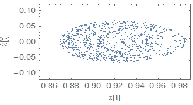
libration points, it is a projection of the orbits from (𝑋, 𝑌, 𝑋)̇ plane to (𝑋, 𝑋)̇ plane, each point represents an orbit about the libration point.
Now, L1and L2 are chosen as an example of the collinear libration points, while L4 and L6 are chosen as an example of the triangular libration points.
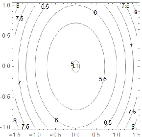
From the results obtained Fig 2 shows periodic orbit about L1, Fig. 3 illustrates the zero-velocity curve and Fig.4 shows a Poincare surface about L1 and Fig 5 shows periodic orbit about L2, Fig. 6 illustrates the zero-velocity curve and Fig.7 shows a Poincare surface about L2. The same for L4, Fig 8 shows the periodic orbit about L4, Fig. 9 shows the zero-velocity curves and Fig.10 Poincare surface about L4. The same for L6 is illustrated in figures 11, 12, and 13.
Table 1: The collinear and non-collinear libration points for the Sun-Earth system and their Jacobi constant C, eccentricity and period of the orbit about each point.
libration points Position X Y
Jacobi constant eccentricity period of the orbit
L1 0.986675 0 2.98435 0.978755 3.13455
L2 1.01201 0 2.98488 0.991976 3.13455
L3 -1.00332 0 2.98463 1.6196 3.13455
L4 0.986675 0.997497 3.3886 0.856303 3.13455
L5 0.986675 -1.0025 3.39508 0.451298 3.13455
L6 0.986675 9.00001*10^-10 2.98435 0.978755 3.13455
Fig. 4. Poincare Surface at L1
Fig.5: the phase space about L2 Fig. 6. Zero Velocity Curve at L2 , C=2.98488
Fig. 8:Phase Space at L4 Fig. 9:Zero Velocity Curve at L4 ,C = 3.3886
Fig. 11: Phase Space at L6 Fig.12:Zero Velocity Curve at L6 ,C = 2.98435
Fig. 13:
Conclusion
In this study, the Variation of Parameters Method is used to obtain the analytical solution of the restricted three-body problem. The obtained solution gives explicit expressions in X, Y depends on the time. The application of these solutions enables us to obtain the libration points and to study the stability of motion about these libration points, the results obtained are in a good agreement with the results obtained by Simmons [13], Kunitsyn[14], Schuerman[15]and Ibrahim[16]. Therefore the variation of the parameter method is a good technique to be applied on the astro-dynamical systems.
Acknowledgements
Praise be to Allah, whose grace is best, I extend my sincere thanks and gratitude to my husband and second to Prof. Muhammad Nader for his generosity to me and my colleague Dr. Ahmed Hafez for all his assistance. Thank you all.
References
[1] Abell,M.L. and Braselton,J.P. Differential equations with Mathematica. Academic Press (2016).
[2] Efroimsky, M. Gauge freedom in orbital mechanics Annals of the New York Academy of Sciences, 1065(1), 346-374. (2005).
[3] Vallado,D. A. in Elsevier Astrodynamics Series (2006 ).
[4] Moulton, F. R. An introduction to celestial mechanics.Courier Corporation (2012).
[5] Lovett, E. O."The theory of perturbations and Lie s theory of contact transformations",The Quarterly Journal of Pure and Applied Mathematics, vol. 30, pages 47 149.(1899).
[6] Oberti, P., and Vienne, A. An upgraded theory for Helene, Telesto, and Calypso. Astronomy & Astrophysics, 397(1), 353-359. (2003).
[7] Vallado, D. A. Perturbed motion. Modern Astrodynamics, 1-22. (2006).
[8] Srivastava, V. K., Kumar, J., and Kushvah, B. S. Halo orbit transfer trajectory design using invariant manifold in the Sun-Earth system accounting radiation pressure and oblateness. Astrophysics and Space Science, 363(1), 17. (2018).
[9] George, B. A. and Frank E. H. In Mathematical Methods for Physicists (Seventh Edition) (2013).
[10] Douskos, C. N. Collinear equilibrium points of Hill s problem with radiation and oblateness and their fractal basins of attraction. Astrophysics and Space Science, 326(2), 263-271. (2010).
[11] Sharma, R. K., and Rao, P. S. Stationary solutions and their characteristic exponents in the restricted three-body problem when the more massive primary is an oblate spheroid. Celestial mechanics, 13(2), 137-149. (1976).
[12] Simmons, J.F.L., McDonald, A.J.C., and Brown, J.C. Celest. Mech. 35,145. (1985).
[13] Kunitsyn, A. L., and Polyakhova, E. N. The restricted photogravitational three-body problem: a modern state. Astronomical and Astrophysical Transactions, 6(4), 283-293. (1995).
[15] Ibrahim, A. H., Ismail, M. N., Zaghrout, A. S., Younis, S. H., and El Shikh, M. O. Lissajous Orbits at the Collinear Libration Points in the Restricted Three-Body Problem with Oblateness. World Journal of Mechanics, 8(06), 242. (2018).
[16] Ismail, M. N., Younis, S. H., and Elmalky, F. M. Modeling sun s radiation e⁄ect on restricted four bodies. NRIAG Journal of Astronomy and Geophysics, 7(2), 208-213. (2018).
[17] Chen, W., Fong, C. C. M., & De Kee, D. Perturbation methods, instability, catastrophe and chaos. World Scienti c (1999).
[18] Palais, R. S., & Palais, R. A. Differential equations, mechanics, and computation (Vol. 51). American Mathematical Soc (2009).
[19] Szebehely, V. Theory of orbits: the restricted problem of three bodies. Yale univ New Haven CT (1967). [20] Ibrahim, A. H., Ismail, M. N., Zaghrout, A. S., Younis, S. H., & El Shikh, M. O. Orbital Motion Around the