Volume 64: Programming and Computer Languages 2013

Volume 64 (2013)

Proceedings of the

XIII Spanish Conference on Programming

and Computer Languages

(PROLE 2013)

Automatic Proving of Fuzzy Formulae with Fuzzy Logic Programming

and SMT

Miquel Bofill, Gin´es Moreno, Carlos V´azquez and Mateu Villaret

19 pages

Guest Editors: Clara Benac Earle, Laura Castro, Lars-iAkeFredlund ManagingEditors:TizianaMargaria,JuliaPadberg,GabrieleTaentzer

Automatic Proving of Fuzzy Formulae with Fuzzy Logic

Programming and SMT

Miquel Bofill1, Gin´es Moreno2, Carlos V´azquez2and Mateu Villaret1

1_{[email protected], [email protected]}

Department of Computer Science, Applied Mathematics and Statistics University of Girona

17071 Girona (Spain)

2_{[email protected], [email protected]}

Department of Computing Systems University of Castilla-La Mancha

02071 Albacete (Spain)

Abstract: In this paper we deal with propositional fuzzy formulae containing sev-eral propositional symbols linked with connectives defined in a lattice of truth de-grees more complex than Bool. We firstly recall an SMT (Satisfiability Modulo Theories) based method for automatically proving theorems in relevant infinitely-valued (includingŁukasiewiczandG¨odel) logics. Next, instead of focusing on sat-isfiability (i.e., proving the existence of at least one model) or unsatsat-isfiability, our interest moves to the problem of finding the whole set of models (with a finite do-main) for a given fuzzy formula. We propose an alternative method based on fuzzy logic programming where the formula is conceived as a goal whose derivation tree contains on its leaves all the models of the original formula, by exhaustively inter-preting each propositional symbol in all the possible forms according the whole set of values collected on the underlying lattice of truth-degrees.

Keywords:Fuzzy Logic Programming; Automatic Theorem Proving; SMT

1

Introduction

Research on SAT (Boolean Satisfiability) and SMT (Satisfiability Modulo Theories) [BSST09] represents a successful and large tradition in the development of highly efficient automatic theo-rem solvers for classic logic. More recently there also exist attempts for covering fuzzy logics, as occurs with the approaches presented in [ABMV12,VBG12]. Moreover, if automatic theorem solving supposes too an starting point for the foundations of logic programming as well as one of its important application fields [Llo87,Sti88,Fit96,Apt90,Bra00], in this work we will show some preliminary guidelines about how fuzzy logic programming can face the automatic proving of fuzzy theorems.

Figure 1: Interpreting a formula with two values for signals/propositionsInandOut.

each propositional symbol, we obtain the following final set of interpretations for the whole formula:

I1 : {In=0,Out=0} ⇒ F=0 I2 : {In=0,Out=1} ⇒ F=1 I3 : {In=1,Out=0} ⇒ F=1 I4 : {In=1,Out=1} ⇒ F=0

com-Figure 2: Interpreting a formula with three values for signals/propositionsInandOut.

posed by just two rules: “i(1) with 1” and “i(0) with 0”, it draws the tree shown in Figure 1, where models I2 and I3 appear in the two central leaves of the tree inside a blue box. Each branch in the tree starts by interpreting variablesInandOut and continues with the evaluation of operators appearing inF.

Note that whereas formula F describes the behaviour of our chip in an “implicit way”, the whole set of modelsI2 andI3 “explicitly” describes how the chip successfully works (any other interpretation not being a model, represents an abnormal behaviour of the chip), hence the im-portance of finding the whole set of models for a given formula.

Assume now that we plan to model an “analogic” version of the chip, where both the input and output signals might vary in an infinite range of values between 0 and 1, such thatOut will simply represent the “complement” ofIn. The new behaviour of the chip can be expressed again by the same previous formula, but taking into account now that connectives involved inFcould be defined in a fuzzy way as follows (see also Figure3afterwards):

x0 = 1−x Product logic’s negation

x∧y = min(x,y) G¨odel logic’s conjunction x∨y = min(x+y,1) Łukasiewicz logic’s disjunction

Here we could use an SMT solver to prove thatF is satisfiable. Following the approach of the work in [ABMV12], it can be easily checked thatF is satisfiable1with the following SMT-LIB script, encoding the previous connectives into SAT modulo linear real arithmetic:

; Set logic: Quantifier Free Linear Real Arithmetic (set-logic QF_LRA)

; min(x,y)

(define-fun min ((x Real) (y Real)) Real (ite (> x y) y x))

; x’ = 1 - x

(define-fun agr_not ((x Real)) Real (- 1 x))

; &G(x,y) = min{x,y}

(define-fun and_godel ((x Real) (y Real)) Real (min x y))

; |L(x,y) = min{x+y,1}

(define-fun or_luka ((x Real) (y Real)) Real (min (+ x y) 1))

; Declaration of variables (declare-fun x () Real) (declare-fun y () Real)

; Ordering relation (assert (>= x 0)) (assert (<= x 1)) (assert (>= y 0)) (assert (<= y 1))

; Formula to check

(assert (= (or_luka (and_godel (agr_not x) y) (and_godel x (agr_not y))) 1))

; Check for satisfiability (check-sat)

It is easy to understand the SMT-LIB syntax of the previous code. Just in case, we recall that theiteexpression corresponds to theif-then-elseconstruct. Note that all necessary connectives are easily encoded as is done in [ABMV12]. It is worth noting that, apart from proving satisfia-bility of a formula, SMT solvers can be used to prove that a formula is a theorem, by checking unsatisfiability of its negation.

we can see in the detailed computations performed along the middle branch of the tree, we have:

(0.50∧0.5)∨(0.5∧0.50) = ((1−0.5)∧0.5)∨(0.5∧0.50) = (0.5∧0.5)∨(0.5∧0.50) =min(0.5,0.5)∨(0.5∧0.50) = 0.5∨(0.5∧0.50) =0.5∨(0.5∧(1−0.5)) =0.5∨(0.5∧0.5) = 0.5∨min(0.5,0.5) =0.5∨0.5

=min(0.5+0.5,1) = min(1,1) =1

Similarly, we can check for instance in the second branch of the tree that{In=1,Out=0.5}is not a model (in fact, our chip can not return a signal of value 0.5 when its input is 1) since:

(10∧0.5)∨(1∧0.50) = ((1−1)∧0.5)∨(1∧0.50) = (0∧0.5)∨(1∧0.50) = min(0,0.5)∨(1∧0.50) = 0∨(1∧0.50) = 0∨(1∧(1−0.5)) =

0∨(1∧0.5) = 0∨min(1,0.5) = 0∨0.5 =

min(0+0.5,1) = min(0.5,1) = 0.5

To finish this section, let us comment some connections between the two main topics of this work, i.e. Fuzzy Logic Programming and Fuzzy SMT, withAnswer Set Programming (ASP), a well-known declarative programming paradigm oriented towards combinatorial search problems which has been recently combined with fuzzy logic [VDV07]. In ASP,answer setsare models computed according to the stable model semantics of logic programming. This introduces non-monotonic reasoning into logic programming, and gives raise to a paradigm that is different from the proof-derivation approach of PROLOG. In [MO09], it is presented an ASP semantics for a kind of fuzzy logic programs very close to MALP, based on the idea of finding models that we also use in this paper when analyzing fuzzy logic formulae with our FLOPER tool. On the other hand, Constraint Satisfaction Problems (CSPs)are mathematical problems defined as a set of objects whose state must satisfy a number of constraints or limitations and hence, SMT and ASP can be roughly thought of as certain forms of CSPs. The translation of answer-set programs into SMT has been considered in [Nie08,JNS09,NJN13]. Also, ASP has been recently combined with SMT in [WZ11]. Although its nonmonotonic form of reasoning is out of the scope of this paper, we are interested in coping with this topic in future extensions of our proposal.

The structure of this paper is as follows. Section 2constitutes the core of our paper and it is divided in three blocks. In sub-section2.1 we present the main features of our fuzzy logic programming environment FLOPER, which are used in sub-section2.2 for analyzing several fuzzy formulae, whereas in sub-section2.3we provide some interesting hints on cost measures associated to our method. Finally, we conclude in Section3by also describing a few number of challenging lines for future research.

2

MALP

,

FLOPER

and Automatic Theorem Proving

In what follows we describe a very simplesubset of theMALP2language(see [MOV04,JMP09] for a complete formulation of this framework), which in essence consists of a first-order lan-guage, L, containing variables, constants, function symbols, predicate symbols, and several

&P(x,y),x∗y |P(x,y),x+y−x∗y ←P(x,y),min(1,x/y)

&G(x,y),min(x,y) |G(x,y),max{x,y} ←G(x,y), (

1 ify≤x x otherwise &L(x,y),max(0,x+y−1) |L(x,y),min{x+y,1} ←L(x,y),min{x−y+1,1}

Figure 3: Conjunctors, disjunctors and implications fromProduct,G¨odelandŁukasiewiczlogics.

(arbitrary) connectives to increase language expressiveness: implication connectives (denoted by←1,←2, . . .); conjunctive connectives (∧1,∧2, . . .), disjunctive connectives (∨1,∨2, . . .), and hybrid operators (usually denoted by @1,@2, . . .), all of them are grouped under the name of

“aggregators”. Although these connectives are binary operators, we usually generalize them as functions with an arbitrary number of arguments. So, we often write @(x1, . . . ,xn) instead of @(x₁, . . . ,@(xn−1,xn)). By definition, the truth function for an n-ary aggregation operator

[[@]]:Ln→Lis required to be monotonous.

Additionally, our languageL contains the values of a lattice(L,≤)and a set of connectives interpreted over such lattice. In general,Lmay be the carrier of any complete bounded lattice where aL-expression is a well-formed expression composed by values ofL, as well as variable symbols, connectives andprimitive operators (i.e., arithmetic symbols such as∗,+,min,etc.). In what follows, we assume that the truth function of any connective @ in L is given by its correspondingconnective definition, that is, an equation of the form @(x1, . . . ,xn),E, whereE

is aL-expression not containing variable symbols apart fromx1, . . . ,xn. For instance, some fuzzy

connective definitions in the lattice([0,1],≤)are presented in Figure3(from now on, this lattice will be calledV along this paper), where labelsL,GandPmean respectivelyŁukasiewicz logic, G¨odel logic andproduct logic (with different capabilities for modeling pessimistic, optimistic andrealistic scenarios, respectively).

This subset of MALP is intended to cope with fuzzy propositional formulae like P∧Q→ P∨Q, where propositionsPandQare interpreted as values of the lattice. To this end, aprogram is defined as a set of rules (also called “facts”) of the form “H with v”, whereH is an atomic formula or atom (usually calledhead), andv is its associated truth degree(i.e., a value of L). More precisely, in our application, heads have always the form “i(v)” and each program rule looks like “i(v)with v”. It is noteworthy to point out that even when we use the same names for constants (building data terms) and truth degrees, the Herbrand Universe of each program and the carrier set of its associated lattice should never be confused, since they are in fact disjoint sets.

A goalis a formula built from atomic formulasB₁, . . . ,Bn (n≥0 ), truth values of L, con-junctions, disjunctions and aggregations, submitted as a query to the system. In this subset of MALP, the atomic formulas of agoalhave always the form “i(P)”, beingPa variable symbol. In this way, when running a simple goal like “i(P)” (as done in Figure4), we could obtain several answers meaning something like “whenP=v, then the resulting truth degree isv”, representing all possible interpretations inLfor propositionPin the original formula.

the following,C[A]denotes a formula whereAis a sub-expression which occurs in the –possibly empty– contextC[]. Moreover,C[A/A0]means the replacement ofAbyA0in contextC[].

Definition 1(Admissible Step) LetQ be a goal and letσ be a substitution. The pairhQ;σi is astate. Given a program P, anadmissible computation is formalized as a state transition system, whose transition relation→ASis defined as the least one satisfying:

hQ[A];σi →AS h(Q[A/v])θ;σ θi

whereAis the selected atom inQ,θ =mgu({H=A})3 and “H with v” inP. Anadmissible

derivationis a sequencehQ;idi→AS· · · →AShQ0;θi.

If we exploit all atoms of a given goal, by applying admissible steps as much as needed during the operational phase, then it becomes a formula with no atoms (aL-expression) which can be then interpreted w.r.t. latticeLas follows.

Definition 2(Interpretive Step and Fuzzy Computed Answer) LetPbe a program,Q a goal andσa substitution. Assume that[[@]]is the truth function of connective @ in the lattice(L,≤) associated toP, such that, for valuesr1, . . . ,rn,rn+1∈L, we have that [[@]](r1, . . . ,rn) =rn+1.

Then, we formalize the notion of interpretive computationas a state transition system, whose transition relation→ISis defined as the least one satisfying:

hQ[@(r1, . . . ,rn)];σi →IS hQ[@(r1, . . . ,rn)/rn+1];σi

Aninterpretive derivationis a sequencehQ;σi→IS· · · →IShQ0;σi. WhenQ0=r∈L, the state

hr;σiis called afuzzy computed answer(f.c.a.) for that derivation.

2.1 The Fuzzy Logic Programming Environment FLOPER

The parser of our FLOPER tool [MMPV10,MMPV11] has been implemented by using the Pro-log language. Once the application is loaded inside a ProPro-log interpreter, it shows a menu which includes options for loading/compiling, parsing, listing and saving MALP programs, as well as for executing/debugging fuzzy goals. Moreover, in [MMPV10] we explain that FLOPER has been recently equipped with new options, called “lat” and “show”, for allowing the possibility of respectively changing and displaying the lattice associated to a given program.

A very easy way to model truth-degree lattices for being included into the FLOPER tool is also described in [MMPV10], according the following guidelines. All relevant components of each lattice are encapsulated inside a Prolog file which must necessarily contain the definitions of a minimal set of predicates defining the set of valid elements (member/1 predicate), the top and bottom elements (top/1andbot/1predicates), the full or partial ordering established among them (leq/2predicate), as well as the repertoire of fuzzy connectives which can be used for their subsequent manipulation. If we have, for instance, some fuzzy connectives of the form &label1 (conjunction), |label2 (disjunction) or @label3 (aggregation) with aritiesn1, n2 andn3

re-spectively, we must provide clauses defining theconnective predicates“and label₁/(n₁+1)”,

Figure 4: A work-session with FLOPER solving goali(P).

“or label₂/(n₂+1)” and “agr label₃/(n₃+1)”, where the extra argument of each predicate is intended to contain the result achieved after the evaluation of the proper connective. Finally, for the purposes of the current work, we also require for each lattice a Prolog fact of the form

members(L)being theLa list containing the set of truth degrees belonging to the modeled lat-tice (or at least a representative subset of them when working with infinite latlat-tices) for being used when interpreting propositional variables of fuzzy formulae. For instance, a lattice defining the simplest notion of binary lattice should implement predicatemember/1with factsmember(0)

andmember(1)(including alsomembers([0,1])) and the Boolean conjunction could be defined by the pair of factsand bool(0, ,0)andand bool(1,X,X).

member(X) :- number(X),0=<X,X=<1. members([0,0.5,1]).

leq(X,Y) :- X=<Y. bot(0). top(1).

and_luka(X,Y,Z) :- pri_add(X,Y,U1),pri_sub(U1,1,U2),pri_max(0,U2,Z). and_godel(X,Y,Z):- pri_min(X,Y,Z).

and_prod(X,Y,Z) :- pri_prod(X,Y,Z).

or_luka(X,Y,Z) :- pri_add(X,Y,U1),pri_min(U1,1,Z). or_godel(X,Y,Z) :- pri_max(X,Y,Z).

or_prod(X,Y,Z) :- pri_prod(X,Y,U1),pri_add(X,Y,U2), pri_sub(U2,U1,Z).

agr_aver(X,Y,Z) :- pri_add(X,Y,U),pri_div(U,2,Z). agr_not(X,Y) :- pri_sub(1,X,Y).

pri_add(X,Y,Z) :- Z is X+Y. pri_min(X,Y,Z) :- (X=<Y,Z=X;X>Y,Z=Y). pri_sub(X,Y,Z) :- Z is X-Y. pri_max(X,Y,Z) :- (X=<Y,Z=Y;X>Y,Z=X). pri_prod(X,Y,Z) :- Z is X * Y. pri_div(X,Y,Z) :- Z is X/Y.

Figure 5: Prolog code for representing latticeV, which models truth degrees in the real interval [0,1]with standard fuzzy connectives.

shown in Figure2.

Note also that we have included definitions for auxiliary predicates, whose names always begin with the prefix “pri ”. All of them are intended to describe primitive/arithmetic operators (in our case +, −, ∗, /, minandmax) in a Prolog style, for being appropriately called from the bodies of clauses defining predicates with higher levels of expressivity (this is the case for instance, of the three kinds of fuzzy connectives we are considering: conjunctions, disjunctions and aggregations).

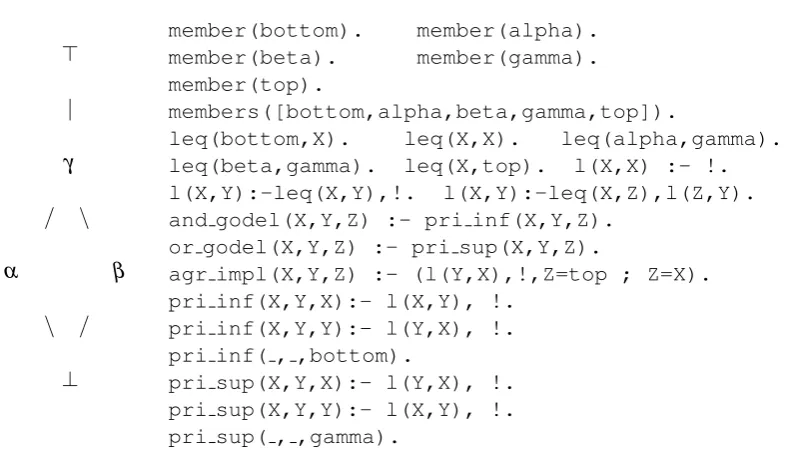
Since till now we have considered two classical, fully ordered lattices (with a finite and infi-nite number of elements, respectively), we wish now to introduce a different case coping with a very simple lattice where not always any pair of truth degrees are comparable. So, consider the following partially ordered latticeFin the diagram of Figure6, which is equipped with conjunc-tion, disjunction and implication connectives based on theG¨odellogic described in Figure3, but with the particularity that now, in the general case, theG¨odel’s conjunction must be expressed as &G(x,y),in f(x,y), where it is important to note that we must replace the use of “min” by “inf”

in the connective definition (and similarly for the disjunction connective, where “max” must be substituted by “sup”).

To this end, observe in the Prolog code accompanying the graphic in Figure 6that we have introduced clauses defining the primitive operators “pri inf/3” and “pri sup/3” which are intended to return theinfimumandsupremumof two elements. Related with this fact, we must point out the following aspects:

>

|

γ

/ \

α β

\ /

⊥

member(bottom). member(alpha). member(beta). member(gamma). member(top).

members([bottom,alpha,beta,gamma,top]).

leq(bottom,X). leq(X,X). leq(alpha,gamma). leq(beta,gamma). leq(X,top). l(X,X) :- !. l(X,Y):-leq(X,Y),!. l(X,Y):-leq(X,Z),l(Z,Y). and godel(X,Y,Z) :- pri inf(X,Y,Z).

or godel(X,Y,Z) :- pri sup(X,Y,Z).

agr impl(X,Y,Z) :- (l(Y,X),!,Z=top ; Z=X). pri inf(X,Y,X):- l(X,Y), !.

pri inf(X,Y,Y):- l(Y,X), !. pri inf( , ,bottom).

pri sup(X,Y,X):- l(Y,X), !. pri sup(X,Y,Y):- l(X,Y), !. pri sup( , ,gamma).

Figure 6: The finite, partially ordered latticeF modeled in Prolog.

• A goal of the form “?- pri inf(alpha,beta,X).”, instead of failing, successfully produces the desired result “X=bottom”.

• Note anyway that the implementation of the “pri inf/3” predicate is mandatory for coding the general definition of “and godel/3” (a similar reasoning fol-lows for “pri sup/3” and “or godel/3” ).

2.2 Some Examples

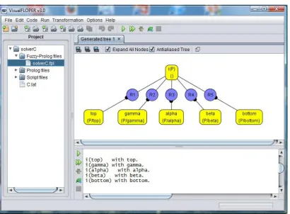
This subset of the MALP language suffices for developing a simple fuzzy theorem prover, where it is important to remark that our tool can cope with different lattices (not only the real interval [0,1]) containing a finite number of elements -marked in “members”- maintaining full or partial ordering among them. Hence, we can use FLOPER for enumerating the whole set of interpreta-tions and models of fuzzy formulae. To this end, only a concrete latticeLis required in order to automatically build a program composed by a set of facts of the form “i(α) with α”, for each α∈L. For instance, the MALP program associated to latticeF in Figure6looks like:

i(top) with top.

i(gamma) with gamma. i(alpha) with alpha.

i(beta) with beta.

i(bottom) with bottom.

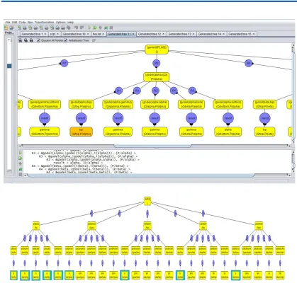
Figure 7: A work-session with FLOPER solving formulaP∨Q(25 interpretations, 9 models).

• IfPis a propositional variable in the original formula, then it is denoted as “i(P)” in the goalF.

• If & is a conjunction of a certain logic “label” in the original formula, then it is denoted as “&label” in goalF.

• For disjunctions, negations and implications, use respectively “|label”, “@no label” and “@im label” inF.

• For other aggregators use “@label” inF.

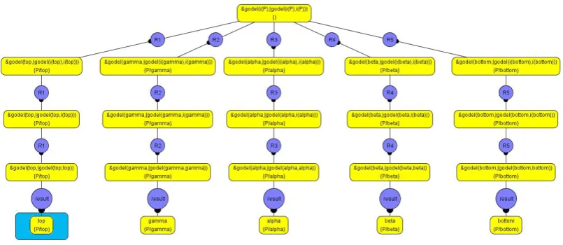
Figure 8: Full proof tree for formulaP∧(P∨P)with 1 model among 5 interpretations.

propositional formulaP∨Q, which is translated into the MALP goal “(i(P) | i(Q))” and after being executed with FLOPER, the tool returns a tree4whose 25 leaves represent the whole set of interpretations (9 of them -inside blue clouds- are models) as seen in Figure7. See also Figure8associated to formulaP∧(P∨P).

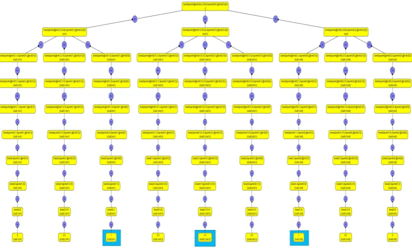
Consider now the more involved formulaP∧Q→P∨Qwhich becomes into the MALP goal “(i(P) & i(Q)) @impl (i(P) | i(Q))”. When interpreted by FLOPER, the system returns the list of answers displayed in Figure 9, having all them the maximum truth degree “top”, which proves that this formula is a tautology, as wanted.

2.3 Some Hints on Cost Measures

We wish to finish this section by providing some comments about cost measures and efficiency. So, given a latticeL, a formulaFand its associated proof treeT, we define the following values:

• vis the number of distinct variables inF.

• v0is the number of occurrences (including repetitions) of variables inF.

• cis the number of connectives inF.

• ris the number of (marked) elements in latticeLgiven by predicate “members”.

And now we have that:

• The width of the treeT, or total number of interpretations ofF, isrv.

4_{Each state contains its corresponding goal and substitution components and they are drawn inside yellow circles.}

Figure 9: Full proof tree for tautologyP∧Q→P∨Q(25 models).

• The number of admissible steps performed on a single branch ofT isv0.

• The number of interpretive steps performed on a single branch ofT isc.

• The depth ofT, or number of computational (admissible/interpretive) steps for each pos-sible interpretation ofFisv0+c.

• An upper bound for the total number of admissible steps inT is|as| ≤(v0−v)rv+ v

∑

i=1 ri.

• An upper bound for the total number of interpretive steps inT is|is| ≤crv.

• An finally, an upper bound for the total number of computational (admissible and

interpre-tive) steps is|T| ≤(c+v0−v)rv+ v

∑

i=1 ri.

Let us come back again to tautologyP∧Q→P∨Qfor which FLOPER displays the whole set of models seen in Figure9, and assume now a more general version with the following shape P1∧. . .∧Pn→P1∨. . .∨Pnfor which we have studied its behaviour in the table of Figure10. In the horizontal axis we represent the numbernof different propositional variables appearing in the formula, whereas the vertical axis refers to the number of seconds5 needed to obtain the whole set of interpretations (all them are models in this case) for the formula. Both the red and blue lines refers to the method just commented along this paper, but whereas the red line indicates that

5 _{The benchmarks have been performed using a computer with processor Intel Core Duo, with 2 GB RAM and}

Figure 10: Behaviour of the method.

the derivation tree has been produced by performing admissible and interpretive steps according Definitions1and2, respectively, the blue line refers to the execution of the Prolog code obtained after compiling with FLOPER the MALP program and goal associated to our intended formula. The results achieved in the figure show that our method has a nice behaviour in both cases, even for formulae with a big number of propositional variables. Of course, the method does not try to compete with SAT techniques (which are always faster and can deal with more complex formulae containing many more propositional variables), but it is important to remark again that in our case, we face the problem of finding the whole set of models for a given formula, instead of only focusing on satisfiability.

3

Conclusions and Future Work

<node> <rule>R0</rule> <goal>or_godel(i(P),i(Q))</goal> <substitution>{}</substitution> <children> <node> <rule>R1</rule> <goal>or_godel(bottom,i(Q))</goal> <substitution>{P/bottom}</substitution> <children> <node> <rule>R1</rule> <goal>or_godel(bottom,bottom)</goal> <substitution>{Q/bottom,P/bottom}</substitution> <children> <node> <rule>result</rule> <goal>bottom</goal> <substitution>{Q/bottom,P/bottom}</substitution> <children> </children> </node> </children> </node> ...

Figure 11: Part of the XML file representing the execution tree shown in Figure7.

(based on “pointing out” just a few number of truth degrees in the infinite space). In this last sense, somehalting rulesandbranch cutsshould be needed (maybe throughalfa cuts) or even it could be interesting to study how to obtain all models of a formula by a constraint (asx+y=1 for the example given in the Introduction about the analogical chip) or a set of constraints. Moreover, we are also interested in reinforcing our techniques by making use of recent advances produced in the field of (fuzzy variants of) ASP.

<root>

<substitution>{Q/top,P/bottom}</substitution> <substitution>{Q/top,P/alpha}</substitution> <substitution>{Q/top,P/beta}</substitution> <substitution>{Q/top,P/gamma}</substitution> <substitution>{Q/bottom,P/top}</substitution> <substitution>{Q/alpha,P/top}</substitution> <substitution>{Q/beta,P/top}</substitution> <substitution>{Q/gamma,P/top}</substitution> <substitution>{Q/top,P/top}</substitution> </root>

Figure 12: XML file obtained after evaluating an XPath query.

conditions (between square brackets‘[]’) on nodes and leaves to restrict the number of answers of the query. For instance, we have used the XPath online toolhttp://www.xpathtester.com/test for executing the query “//node[goal=’top’]/substitution” against the XML file shown in Figure11, which was generated by FLOPER when producing the proof tree drawn in Figure7, thus returning as output the new XML document listed in Figure12. As illustrated in Figure11, note that the XML files representing proof trees exported by FLOPER, are always rooted with thenodelabel, whose children are based on four finds of ‘tags’ (this structure is nested as much as needed):

• rule, which indicates the program rule evaluated to reach the current node (the virtual ruleR0is pointed out only in the initial node),

• goal, which contains the MALP expression under evaluation, that is, the formula that the system is trying to prove on its current initial/intermediate/final step. Note that, when in our example such value istop, then we have found a model, where the values assigned to the propositional symbols of the formula are collected in the following tag...

• substitution, which accumulates the variable bindings performed along a fuzzy logic derivation (i.e., chain of computational steps along a branch of the execution tree) and whose meaning in our target setting, reveals the way of interpreting the propositions con-tained on a formula for obtaining its models (see Figure 12, where the nine solutions labeled with this tag and reported in the output XML document, indicate each one the truth values for the propositional variables that satisfy the formula with the maximum truth degree), and finally

• children, which contains the set of underlying nodes of the tree in a nested way.

Acknowledgements: This work has been partially supported by the EU (FEDER), and the Spanish MINECO Ministry (Ministerio de Econom´ıa y Competitividad) under grants TIN2012-33042 and TIN2013-45732-C4-2-P. Moreover, Carlos V´azquez and Gin´es Moreno received grants for International mobility from the University of Castilla-La Mancha (CYTEMA project and Vicerrectorado de Profesorado).

Bibliography

[ABMV12] C. Ans´otegui, M. Bofill, F. Many`a, M. Villaret. Building Automated Theorem Provers for Infinitely-Valued Logics with Satisfiability Modulo Theory Solvers. In Proceedings of the 42nd IEEE International Symposium on Multiple-Valued Logic, ISMVL 2012. Pp. 25–30. 2012.

[ALM11] J. Almendros-Jim´enez, A. Luna, G. Moreno. A Flexible XPath-based Query Lan-guage Implemented with Fuzzy Logic Programming. In Bassiliades et al. (eds.), Proceedings of 5th International Symposium on Rules: Research Based, Industry Focused, RuleML’11. Barcelona, Spain, July 19–21. Pp. 186–193. Springer Verlag, LNCS 6826, 2011.

[ALM12] J. Almendros-Jim´enez, A. Luna, G. Moreno. Fuzzy Logic Programming for Imple-menting a Flexible XPath-based Query Language.Electronic Notes in Theoretical Computer Science282:3–18, 2012.

[ALMV13] J. Almendros-Jim´enez, A. Luna, G. Moreno, C. V´azquez. Analyzing Fuzzy Logic Computations with Fuzzy XPath. In Fredlund and Castro (eds.), Actas de las XIII Jornadas sobre Programaci´on y Lenguajes, PROLE’13, Jornadas SISTEDES, Madrid, Spain, September 18-20. Pp. 136–150 (“work in progress” track, extended version submitted to ECEASST). Universidad Complutense de Madrid (ISBN: 978-84-695-8331-9), 2013.

[Apt90] K. R. Apt. Logic Programming. In Leewen (ed.), Handbook of Theoretical Com-puter Science. Volume B: Formal Models and Semantics, chapter 10, pp. 493–574. MIT Press, Massachusetts Institute of Technology, USA, 1990.

[BBC+07] A. Berglund, S. Boag, D. Chamberlin, M. Fernandez, M. Kay, J. Robie, J. Sim´eon. XML path language (XPath) 2.0.W3C, 2007.

[Bra00] I. Bratko.Prolog Programming for Artificial Intelligence. Addison Wesley, Septem-ber 2000.

[BSST09] C. W. Barrett, R. Sebastiani, S. A. Seshia, C. Tinelli. Satisfiability Modulo Theo-ries. InHandbook of Satisfiability. Frontiers in Artificial Intelligence and Applica-tions 185, pp. 825–885. IOS Press, 2009.

[JMM+13] P. Juli´an, J. Medina, P. Morcillo, G. Moreno, M. Ojeda-Aciego. An Unfolding-Based Preprocess for Reinforcing Thresholds in Fuzzy Tabulation. InAdvances in Computational Intelligence - Proc of the 12th International Work-Conference on Artificial Neural Networks, IWANN 2013. Tenerife, Spain, June 12-14. Pp. 647– 655. Springer Verlag, LNCS 7902, PART I, 2013.

[JMP09] P. Juli´an, G. Moreno, J. Penabad. On the Declarative Semantics of Multi-Adjoint Logic Programs. InProceedings of the 10th International Work-Conference on Ar-tificial Neural Networks, IWANN’09. Salamanca, Spain, June 10-12. Pp. 253–260. Springe Verlag, LNCS 5517, 2009.

[JNS09] T. Janhunen, I. Niemel¨a, M. Sevalnev. Computing Stable Models via Reductions to Difference Logic. In Erdem et al. (eds.),Proc. of the 10th International Conference on Logic Programming and Nonmonotonic Reasoning, LPNMR 2009, Potsdam, Germany, September 14-18. Pp. 142–154. Springer Verlag, LNCS 5753, 2009.

[Llo87] J. Lloyd. Foundations of Logic Programming. Springer-Verlag, Berlin, 1987. Sec-ond edition.

[LMM88] J. L. Lassez, M. J. Maher, K. Marriott. Unification Revisited. In Minker (ed.), Foun-dations of Deductive Databases and Logic Programming. Pp. 587–625. Morgan Kaufmann, Los Altos, California, 1988.

[MMPV10] P. Morcillo, G. Moreno, J. Penabad, C. V´azquez. A Practical Management of Fuzzy Truth Degrees using FLOPER. In al. (ed.),Proceedings of 4th Intl Symposium on Rule Interchange and Applications, RuleML’10. Washington, USA, October 21–23. Pp. 119–126. Springer Verlag, LNCS 6403, 2010.

[MMPV11] P. Morcillo, G. Moreno, J. Penabad, C. V´azquez. Fuzzy Computed Answers Col-lecting Proof Information. In al. (ed.), Advances in Computational Intelligence. Proceedings of the 11th International Work-Conference on Artificial Neural Net-works, IWANN 2011. Torremolinos, Spain, June 8-10. Pp. 445–452. Springer Ver-lag, LNCS 6692, 2011.

[MMPV12] P. J. Morcillo, G. Moreno, J. Penabad, C. V´azquez. Dedekind-MacNeille comple-tion and Cartesian product of multi-adjoint lattices. Int. J. Comput. Math. 89(13-14):1742–1752, 2012.

[MO09] N. Madrid, M. Ojeda-Aciego. On Coherence and Consistence in Fuzzy Answer Set Semantics for Residuated Logic Programs. In Ges`u et al. (eds.), Proc. of the 8th International Workshop on Fuzzy Logic and Applications, WILF 2009. Palermo, Italy, June 9-12. Pp. 60–67. Springer Verlag, LNCS 5571, 2009.

[MOV04] J. Medina, M. Ojeda-Aciego, P. Vojt´aˇs. Similarity-based Unification: a multi-adjoint approach.Fuzzy Sets and Systems146:43–62, 2004.

[NJN13] M. Nguyen, T. Janhunen, I. Niemel¨a. Translating Answer-Set Programs into Bit-Vector Logic. In Tompits et al. (eds.), Proc. of the 19th International Conference on Applications of Declarative Programming and Knowledge Management, INAP 2011. Vienna, Austria, September 28-30. Pp. 95–113. Springer Verlag, LNCS 7773, 2013.

[Sti88] M. E. Stickel. A Prolog technology theorem prover: Implementation by an extended Prolog compiler.Journal of Automated reasoning4(4):353–380, 1988.

[VBG12] A. Vidal, F. Bou, L. Godo. An SMT-Based Solver for Continuous t-norm Based Logics. In Proceedings of the 6th International Conference on Scalable Uncer-tainty Management, SUM 2012. Marburg, Germany, September 17-19. Pp. 633– 640. Springer Verlag, LNCS 7520, 2012.

[VDV07] D. Van Nieuwenborgh, M. De Cock, D. Vermeir. An introduction to fuzzy answer set programming.Annals of Mathematics and Artificial Intelligence50(3-4):363– 388, 2007.