G. ANKAMMA RAO
Data Structures
Data structures
Stack
Queue – Circular Queue, De-Queue
& Priority queue
Linked List- SLL and DLL
Donald D. Chamberlin
Data Structures
A Data Structure is a mathematical or logical way of organizing data in the memory that consider not only the items stored but also the relationship to each other and also it is characterized by accessing methods.
Data Structure is a collection of data items organized in specific manner. And also we define methods to store and retrieve data elements.
Data type is called as data structure, generally integer, char, float etc.. are called as the primitive data types and these are also called as primitive data structures. Using this primitive data structures we can construct simple data structures (Arrays).
Using primitive and simple data structures we construct complex data structures. The complex data structures are stack, queue, linked list, trees and graphs.
As stated earlier, the following operations are done on data structures: Data organization or clubbing
Accessing technique
Manipulating selections for information.
Example: Stack, Queue, Linked List, Trees and graphs.
Data structures have been classified into two ways. They are
Linear
Non-Linear
Linear Data Structure
In linear data structures, values are arranged in linear fashion. Arrays, linked lists, stacks and queues are examples of linear data structures in which values are stored in a sequence.
Non-Linear Data Structure
Chapter
Stack
Stack is an important tool in programming languages. Stack is one of the most essential linear data structures. Stack is a memory portion, which is used for storing the elements. The elements are stored based on the principle of Last-In-First-Out (LIFO). In the stack the elements are kept one above the other and its size is based on the memory.
Size = 5 4 3 2 1 0 Top = -1
Top
The Top of the pointer points to the top element in the stack. The top of the stack indicates its door from where elements are entered or deleted. The stack top is used to verify stack's current position, i.e. underflow, overflow, etc. The initial value of the top in stack is -1.
Operations on Stack
The following fundamental operations on stack can be carried out through static implementation called array implementation. We will perform the following operations on the stack:
Create a stack
Insert (push) an element in the stack
Delete (pop) an element from the stack
These are explained as follows
Create
Create an empty stack with some size.
Push
The process of inserting data element into the stack is called as push.Initially top is set to ‘-1’. To insert an element into the stack first we need to check the following condition.
if(top==size-1) {
Stack is overflow; // stack is full }
else {
Otherwise increment the top and insert the data element in that location;
}
Consider a stack with size is 5.
size = 5
4 3 2 1 0
top = -1
push(2) 4 3 2 1 0
top = 0
push(4) 4 3 2 1 0
top = 1
Pop
The process of deleting data element from the stack is called pop. To pop an element from the stack first we need to check the following condition.
if(top==-1) {
Stack is underflow; }
else {
Delete an element from the stack; }
If the stack is not empty retrieve the top of the stack element and store it in variable ‘x’ and then decrement the top by ‘1’.
4 3 2 1 0
top = 4
pop(10) 4 3 2 1 0
x = 10 top = 3
pop(8) 4 3 2 1 0
x = 8 top = 2
pop(6) 4 3 2 1 0
x = 6 top = 1
pop(4) 4 3 2 1 0
x = 4 top = 0
pop(2) 4 3 2 1 0
x = 2 top = -1
After deleting all the elementstop = -1it specifies that stack is empty.
Stack Underflow-Any attempt to delete an element from already empty stack results into Stack Underflow.
If stack contains elements display it, otherwise display stack is empty.
// Java program to implement stack
import java.io.*; class Stack
{
int max, stk[], top; Stack(int size)
{
max = size;
stk = new int [max]; top = -1;
}
void push(int ele) {
if (top == (max-1)) {
System.out.println( "Stack is full "); }
else {
++top ;
stk[top]=ele;
System.out.println( stk[top]+" is inserted successfully"); }
}
void pop() {
int ele;
System.out.println( stk[top]+" element is deleted "); top--;
}
}
void display() {
if (top == -1)
System.out.println( "Stack is EMPTY "); else
{
for (int i = top; i>=0; i--) {
System.out.println( stk [i] +"Stack elements are "); }
}
}// display()
}// Stack class
class StackImp {
public static void main (String a[]) throws IOException {
Stack s = new Stack (5);
DataInputStream d = new DataInputStream(System.in); System.out.println("1 --- push");
System.out.println("2 --- pop"); System.out.println("3 --- display"); System.out.println("4 --- exit"); int ch;
do {
switch(ch) {
case 1:
System.out.println( " Enter Stack element "); int ele = Integer.parseInt(d.readLine()); s.push(ele);
break; case 2:
s.pop(); break; case 3:
s.display(); break;
case 4: System.out.println( " Exit from stack "); break;
}
}while (ch !=4); }// main close }// class close
Applications of Stack
Generally mathematical expressions are represented in three ways:
Infix Expression- In this the operator is placed in between the two operands.
Ex: A + B, A-B, (A+B) * (C-D)
Prefix Expression - In this the operator is placed before the two operands.
Ex: + AB, -AB, * + AB–CD
Postfix Expression - In this the operator is placed after the two operands
Ex: AB +, AB-, AB+ CD - *
Queue
Queue is a Linear Data Structure in which the data element is inserted at one end is called as Rear
end. The data element is deleted from another end is called Front end.
Queue is like a stack, except that in a queue the first item inserted is the first to be removed (First-In-First-Out, FIFO), while in a stack, as we’ve seen, the last item inserted is the first to be removed (LIFO). A
queue works like the line at the student fee counter:
The first person to join the rear of the line is the first person to reach the front of the line and pay a fee. The last person to line up is the last person to buy a fee.
Figure shows how such a queue looks.
Queue follows FIFO (First In First Out) i.e.In Queue the first inserted element is comes out first.
Front Rear
0 1 2 3 4
size = 5
Operations of Queue: Create:
It is used to create empty queue.
Insert:
Before inserting the data element in Queue first of check the condition (rear == size-1), if it is true that means Queue is overflow (full). Otherwise increment the rear and insert the data element in that location.
Example: Initially front and rear are set to‘-1’.
size = 5
0 1 2 3 4 front = -1
rear = -1
insert(2) 2
0 1 2 3 4 front = -1
rear = rear +1 (rear = -1+1 = 0)
i.e. rear = 0
insert(4) 2 4
insert(6)
2 4 6
0 1 2 3 4 front = -1
rear = 2
insert(8)
2 4 6 8
0 1 2 3 4 front = -1 rear = 3
insert(10)
2 4 6 8 10
0 1 2 3 4 front = -1
rear = 4
Now rear == size-1 (i.e.4). it means the queue is full. No more insertion is not possible in this stage.
Delete:
Before deleting data element first of all check the condition (front == rear). If it is true it means that queue is underflow. Otherwise increment front and delete the data element in that location.
size = 5
2 4 6 8 10
0 1 2 3 4 front = -1 rear = 4
delete(2)
4 6 8 10
0 1 2 3 4 (front = front +1)
=> -1+1 = 0 i.e. front = 0 rear = 4
x= 2
delete(4)
6 8 10 0 1 2 3 4
front = 1 rear = 4 x= 4
delete(6)
8 10 0 1 2 3 4
front = 2 rear = 4 x = 6
delete(8)
10 0 1 2 3 4
front = 3 rear = 4 x = 8
delete(10)
0 1 2 3 4 front = 4
rear = 4 x = 10
Display:
It is used to display the elements in the queue.
After deleting the entire elements front == size-1 (i.e. 4); it means that queue is empty.
General Example
Applications
Queue is used in simulation; Simulation is nothing but a predefined tool to examine the behaviour of a system.
Queue is used in time sharing computer system. Used find path in BFS in a graph
Queue is implemented by using arrays and linked list
Java program to implement Queue
import java.io.*; class Queue
{
int max, que[], front,rear; Queue(int size)
{
max = size;
que = new int [max]; front = rear = -1; }
void insert(int ele) {
if (rear == (max-1)) {
System.out.println( "Queue is full "); }
else {
++rear ;
que[rear]=ele;
System.out.println( que[rear]+" is inserted successfully \n ");
void delete() {
int ele;
if (front == -1)
System.out.println( "Queue is Empty \n "); else
{
ele= que[front];
System.out.println( ele+" Element is deleted \n");
if (front==rear) {
front=rear=-1; }
else
front++; }
}
void display() {
if (front == -1)
System.out.println( " Queue is empty "); else
{
for (int i = front; i<=rear; i++) {
System.out.println( " \t " + que [i]); }
} }
}
class QueueImp {
Queue q = new Queue (5);
DataInputStream d = new DataInputStream(System.in); System.out.println("1 --- Insert");
System.out.println("2 --- Delete"); System.out.println("3 --- Display"); System.out.println("4 --- Exit"); int ch;
do {
System.out.println( "Enter your option: "); ch =Integer.parseInt(d.readLine());
switch(ch) {
case 1:
System.out.println( "Enter Queue element "); int ele = Integer.parseInt(d.readLine()); q.insert(ele);
break; case 2:
q.delete(); break;
case 3:
q.display(); break;
case 4: System.out.println( "Exited from Queue "); break;
}
}while (ch !=4); }
}
Circular Queue
Problem in Queue
For example take a queue with size =3 size = 3
0 1 2 front = -1 rear = -1
insert(5) 5
0 1 2 front = -1 rear = 0
insert(10) 5 10 0 1 2
front = -1 rear = 1
insert(15) 5 10 15 0 1 2 front = -1 rear = 2
delete(5) 10 15 0 1 2
front = 0 rear = 2 x = 5
delete(10) 15 0 1 2
front = 1 rear = 2 x = 10
is possible. This problem is avoided by Circular Queue.
Circular Queue
In circular Queue we insert the data element after rear = size-1. Here we move circularly to insert or delete data elements. It is simply called as circular array.
In circular queue front and rear initially set to zero.
front rear
size = 5
Operations of Circular Queue: Create:
It is used to create empty circular queue.
Insert:
Before inserting the data element in Queue first of check the condition (rear == size-1), if it is true the Queue is overflow (full). Otherwise insert the data element in that location and increment the rear.
Ex: Initially front and rear are set to ‘0’
size = 5
0 1 2 3 4 front = 0 rear = 0
insert(2) 2
0 1 2 3 4 front = 0
rear = 0
insert(4) 2 4
0 1 2 3 4 front = 0
rear = 1
insert(6)
2 4 6
0 1 2 3 4 front = 0
insert(8)
2 4 6 8
0 1 2 3 4 front = 0
insert(10)
2 4 6 8 10
true circular queue is underflow (empty), otherwise delete the data element in that location and increment the front.
size = 5
2 4 6 8 10
0 1 2 3 4 front = 0 rear = 4
delete(2)
4 6 8 10
0 1 2 3 4 x= 2 front = 1 rear = 4
delete(4)
6 8 10 0 1 2 3 4
x= 4 front = 2 rear = 4
delete(6)
8 10 0 1 2 3 4
x = 6 front = 3 rear = 4
delete(8)
10 0 1 2 3 4
x = 8 front = 4 rear = 4
delete(10)
0 1 2 3 4 x = 10
front = 4 rear = 4
After deleting the entire elements front == size-1 (i.e. 4); it means that queue is empty.
Display:
It is used to display the elements in the queue.
The following diagram shows how to insert data element in circular queue from the front end.
De-Queue
Initially front and rear are set to ‘-1’.
Insertion from Front Insertion from Rear
Deletion from front Deletion from Rear
Operations of De-Queue:
a) Insertion from rear
For example consider a queue with size = 5. Here queue is empty. Therefore insertion of front is identical to insertion of rear. For example the data element is inserting from rear end. i.e increment the rear and insert the data element in that location.
Insertion of
(2)-insert(2) 2
0 1 2 3 4 front = -1
rear = rear +1 (rear = -1+1 = 0)
i.e. rear = 0
Insertion of
(4)-Here queue is not empty and front == -1. Therefore insertion from the front not possible. So insert the data element from the rear end. i.e. increment the rear and insert the data element in that location.
insert(4) 2 4
0 1 2 3 4 front = -1
rear = 1
Insertion of
(6)-size = 5
Insert(6)
2 4 6
0 1 2 3 4 front = -1
rear = 2
Insertion of
(8)-Here rear≠ size -1. Increment the rear and insert the data element in that location. Insert(8)
2 4 6 8
0 1 2 3 4 front = -1
rear = 3
Insertion of
(10)-Here rear≠ size -1. Increment the rear the insert the data element in that location. Insert(10)
2 4 6 8 10
0 1 2 3 4 front = -1
rear = 4
Insertion of
(12)-Here rear == size -1.
Therefore De-Queue is overflow and also insertion from the front is not possible because queue is not empty and front=-1
b) Deletion from Rear:
Consider a queue as follows;
2 4 6 8 10
0 1 2 3 4 front = -1
rear = 4 Here front≠rear.
delete(10)
2 4 6 8
0 1 2 3 4 x = 10
front = -1 rear = 3
Again front≠ rear, delete the data element and decrement rear by ‘1’.
delete(8)
2 4 6
0 1 2 3 4 x=8
front = -1 rear = 2
c) Deletion from front:
Consider Queue as follows
2 4 6
0 1 2 3 4 front = -1
rear = 2
Here front ≠ rear, deletion is possible from front end. So increment the front and delete the date element in that location.
delete(2) 4 6
0 1 2 3 4 front = 0
delete(4) 6
0 1 2 3 4 front = 1
rear = 2 x=4
Here queue contains only one element and is deleted by using either end.
d) Insertion from front:
Consider a queue as follows;
6
0 1 2 3 4 front = 1
rear = 2
Here queue isnot empty and front is not equal to ‘-1’. So insertion from front is possible. Insert the element then decrement the front by ‘1’.
Insert (12) 12 6
0 1 2 3 4 front = 0
rear = 2
Again queue is not empty and front≠-1. Insert the data element and decrement front by ‘1’.
Insert(14) 14 12 6
0 1 2 3 4 front = -1
rear = 2
Now further insertion is not possible from the front because front == -1.
Note: Insertion from front is possible only in two cases.
1. Queue is empty. i.e. front == rear
Priority Queue
Priority Queue is a queue, in this insertions are done as a normal queue and deletions are done according to some priority.
For example use the following two operations:
pq_mindel():-Using this operation we find the minimum element in the queue and deleted it from queue. For
example queue size is 5 and initially front and rear set to ‘-1’ and the following 5 elements are inserted;
4 6 2 10 8
0 1 2 3 4 front = -1
rear = 4
Now in this operation data element ‘2’ is deleted and will produce the output as 4 6 10 8.
pq_maxdel():-Using this operation we find the maximum element in the queue and deleted it from the queue. For example consider queue size is 5 and the following 5 elements are inserted;
4 6 2 10 8
0 1 2 3 4 front = -1
rear = 4
Now in this operation data element ‘10’ is deleted and will produce the output as 4 6 2 8.
pq_min or pq_max contains two major issues.
To identy minimum or maximum element.
Shuffle the array.
After shuffling the array, the succeeding elements must be shifted to one position left and also the rear
parts.
The first part of the node is called as data part and the second part is address part (next part), this is shown in below.
Root/Head Node
The data or information part contains the actual data element and the address or next or link part contains the address part of its next node.
The general structure of a Single Linked List is as follows.
Root/Head
1000 2000 3000
We can identify the first node of a Single Linked List by using the head pointer. In this, the head pointer always points to the first node of a Single Linked List. If there are no elements in a Single Linked List the head pointer points to a null value.
Linked list uses external pointer called as root or head. It contains the first node address and using this we access the entire list. i.e. root contains the address of the first node using this we access first node and second node is accessed by using next address field of first node and so on. The last node next address field contains the NULL value. It is not any valid address; it specifies only the end of the list.
In general, we can able to perform the following operations on a Single Linked List.
Insertion of node at beginning.
Insertion of node at end.
Insertion of node at middle.
Deletion of node at beginning.
Deletion of node at end.
Deletion of node at middle.
These are explained below…..
Assume that the newly inserted node is q.
node q=new node();
a) Insertion at beginning
In this method insertion is possible at beginning; for example we consider the linked list as below.
10 2000 20 3000 30 NULL
Root/Head q
1000 2000 3000
Step 1: Create an empty node (p)
p
500 Step 2: Storedata ‘5’in node (p).
p
500 Step 3: Assign root tonode ‘p’.
Root/Head p
500 Step 4: Assign next (p) to q
Root/Head p q
500 1000 2000 3000
b) Insertion of node at end
Using this method we can insert a node with information 40 at the end of the list. For example consider the following linked list.
Root/Head
1000 2000
q
3000
Inserting node r at end
5 1000 10 2000 20 3000 30 NULL
5
10 2000 20 3000 30 NULL
5
Step 4: Assign next (q) to r
Root/Head
1000 2000 3000
q r
4000
c) Insertion of node at middle
Using this method we can insert a node with information 40 at the end of the list. For example consider the following linked list.
Root/Head
1000
p
2000
r
3000
Inserting node q in between p and r
Step 1: Create a node (q)
Step 2: Insertdata ‘25’ into node (q) Step 3: Assign next (p) to q.
Step 4: Assign next (q) to r.
Root/Head
1000
p q
2000 2500
r
3000
d) Deletion of node at beginning
In this method we can delete the beginning node. For example consider a list as follows;
Root/Head p
1000 2000 3000
Deleting node p
Step 1: Assign root to next (p)
Step 2: deletedata ‘10’from node (p) Step 3: Remove node from the list
10 2000 20 3000 30 4000 40 NULL
10 2000 20 3000 30 NULL
10 2000 20 2500 25 3000 30 NULL
Root/Head
2000 3000
e) Deletion of node at ending
In this method we can delete the node at end of the list. For example consider a list as follows;
Root/Head
1000
q
2000
r
3000
Deleting node r
Step 1: Assign NULL to next (q)
Step 2: delete data ‘30’ from node (r) Step 3: Remove node from the list
Root/Head
1000 2000
f) Deletion of node from middle
In this method we can delete the node at middle of the list. For example consider a list as follows;
Root/Head p
1000
q
2000
r
3000
Deleting node q
Step 1: Assign next (p) to next (q)
Step 2: delete data ‘20’ from node(r) Step 3: Remove node from the list
20 3000 30 NULL
10 2000 20 3000 30 NULL
10 1000 20 NULL
Doubly Linked List (DLL)
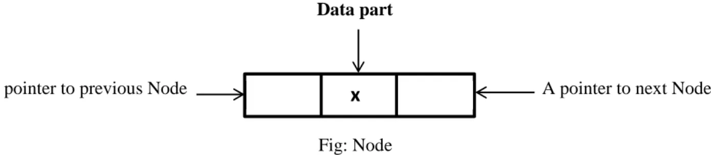
Doubly Linked List is a linear data structures. In DLL each contains the three parts. DLL is a Linear
Data Structure.
A pointer to previous node called as left. Data part.
A pointer to next node called as right.
Data part
A pointer to previous Node A pointer to next Node
Fig: Node
DLL contains external pointer to point the first node address and also first node left pointer and last node right pointer must be set to NULL. This is shown in the following diagram.
Root
1000 2000 3000 4000
If the DLL contains only one node then its left and right pointers must be set to NULL.
Operations of DLL
a) Insertion of node at Beginning
Consider the following DLL
Insertion of node p 10000
Step – 1: Create a node (p) --- p Step - 2: Insert data ‘2’ in ‘p’.
---Step - 3: Assign right (p) to root---Step – 4: Assign Left (p) to NULL---Step – 5: Assign left (root) to p
Step – 6 : Assign root to
p---Root
2000 3000 4000
x
NULL 2 2000 1000 4 3000 2000 6 4000 3000 8 NULL
2
NULL 4 3000 2000 6 4000 3000 8 NULL
2 2000
NULL 2 2000 2000
After insertion node at beginning the DLL is; Root
1000 2000 3000 4000
b) Insertion of node at end
Consider the following DLL Root
2000 3000
Q
4000
Insertion of node r at end
Step – 1: Create a node (r)
Step - 2: Insert data ‘10’ in ‘r’.
Step - 3: Assign right (r) to NULL Step – 4: Assign right (q) to r Step – 5 assign left(r) to q
After inserting node at end the DLL is Root
2000 3000
q
4000
r
5000
c) Insertion of node at middle
Consider the following DLL Root
2000
P
3000
r
4000
Insertion of node q in between p and r
Step – 1: Create a node (q)
Step - 2: Insert data ‘7’ in ‘q’.
NULL 2 2000 1000 4 3000 2000 6 4000 3000 8 NULL
NULL 4 3000 2000 6 4000 3000 8 5000 4000 10 NULL NULLNULL
NULL 4 3000 2000 6 4000 3000 8 NULL
After inserting node at end the DLL is;
Root
2000
p
3000
q
3500
r
4000
d) Deletion of node at Beginning
Consider the following DLL Root p
1000 2000 3000 4000
Deletion of node p
Step – 1: delete 2 from p
Step - 2: Assign root to next (p) Step - 3: Assign left (root) NULL Step – 4: remove node ‘p’.
After Deletion of node at beginning the DLL is; Root
2000 3000 4000
e) Deletion of node at End
Consider the following DLL Root
1000 2000
q
3000
r
4000
Deletion of node r
Step – 1: delete 8 from r
Step - 2: Assign right (q) to NULL Step – 3: remove node ‘r’.
After Deletion of node at end the DLL is;
NULL 4 3000 2000 6 3500 3000 7 4000 3500 8 NULL NULLNULL
NULL 2 2000 1000 4 3000 2000 6 4000 3000 8 NULL
NULL 4 3000 2000 6 4000 3000 8 NULL
Root
1000 2000
q
3000
f) Deletion of node in middle
Consider the following DLL Root
1000
p
2000
q
3000
r
4000
Deletion of node q
Step – 1: delete 6 from q
Step -2: Assign right (p) to r Step -3: Assign left (r) to p Step – 4: remove node ‘q’. After Deletion of node in middle the DLL is
Root
1000
P
2000
r
4000
NULL 2 2000 1000 4 3000 2000 6 NULL
NULL 2 2000 1000 4 3000 2000 6 4000 3000 8 NULL