DSCOVR: Randomized Primal-Dual Block Coordinate Algorithms for Asynchronous Distributed Optimization

DSCOVR: Randomized Primal-Dual Block Coordinate Algorithms

for Asynchronous Distributed Optimization

Lin Xiao [email protected]

Microsoft Research AI Redmond, WA 98052, USA

Adams Wei Yu [email protected]

Machine Learning Department, Carnegie Mellon University Pittsburgh, PA 15213, USA

Qihang Lin [email protected]

Tippie College of Business, The University of Iowa Iowa City, IA 52245, USA

Weizhu Chen [email protected]

Microsoft AI and Research Redmond, WA 98052, USA

Editor:Francis Bach

Abstract

Machine learning with big data often involves large optimization models. For distributed optimiza-tion over a cluster of machines, frequent communicaoptimiza-tion and synchronizaoptimiza-tion of all model parameters (optimization variables) can be very costly. A promising solution is to use parameter servers to store different subsets of the model parameters, and update them asynchronously at different machines using local datasets. In this paper, we focus on distributed optimization of large linear models with convex loss functions, and propose a family of randomized primal-dual block coordinate algorithms that are especially suitable for asynchronous distributed implementation with parameter servers. In particular, we work with the saddle-point formulation of such problems which allows simultaneous data and model partitioning, and exploit its structure by doubly stochastic coordinate optimization with variance reduction (DSCOVR). Compared with other first-order distributed algorithms, we show that DSCOVR may require less amount of overall computation and communication, and less or no synchronization. We discuss the implementation details of the DSCOVR algorithms, and present numerical experiments on an industrial distributed computing system.

1. Introduction

Algorithms and systems for distributed optimization are critical for solving large-scale machine learning problems, especially when the dataset cannot fit into the memory or storage of a single machine. In this paper, we consider distributed optimization problems of the form

minimize w∈Rd

1

m

m X

i=1

f_i(X_iw)+g(w), (1)

whereXi ∈RNi×dis the local data stored at theith machine, fi :RNi →Ris a convex cost function associated with the linear mappingX_iw, andg(w) is a convex regularization function. In addition,

we assume thatgis separable, i.e., for some integern> 0, we can write

g(w) = n X

k=1

gk(wk), (2)

wheregk :Rdk → R, andwk ∈ Rdk for k = 1, . . . ,n are non-overlapping subvectors ofw ∈ Rd withPn

k=1dk = d (they form a partition ofw). Many popular regularization functions in machine learning are separable, for example,g(w)= (λ/2)kwk₂2org(w) =λkwk₁for someλ >0.

An important special case of (1) is distributed empirical risk minimization (ERM) of linear predictors. Let (x₁,y₁), . . . ,(xN,yN) be N training examples, where each xj ∈ Rd is a feature vector andyj ∈Ris its label. The ERM problem is formulated as

minimize w∈Rd

1

N

N X

j=1

φj xTjw +

g(w), (3)

where eachφj :R→Ris a loss function measuring the mismatch between the linear predictionxT_jw and the labelyj. Popular loss functions in machine learning include, e.g., for regression, the squared

lossφj(t) =(1/2)(t−yj)2, and for classification, the logistic lossφj(t)=log(1+exp(−yjt))where

yj ∈ {±1}. In the distributed optimization setting, the N examples are divided intomsubsets, each stored on a different machine. For i = 1, . . . ,m, letI_i denote the subset of 1, . . . ,

N stored at

machineiand letNi = |Ii| (they satisfyPm_i=1Ni = N). Then the ERM problem (3) can be written in the form of (1) by lettingX_iconsist ofxT_j with j∈ I_ias its rows and defining f_i :RNi _→Ras

fi(uIi) = m N

X

j∈Ii

φj(uj), (4)

whereuI_i ∈RNi is a subvector of_u∈RN, consisting of_u

jwith j ∈ Ii.

The nature of distributed algorithms and their convergence properties largely depend on the model of the communication network that connects themcomputing machines. A popular setting in

the literature is to model the communication network as a graph, and each node can only communicate (in one step) with their neighbors connected by an edge, either synchronously or asynchronously (e.g., Bertsekas and Tsitsiklis, 1989; Nedić and Ozdaglar, 2009). The convergence rates of distributed algorithms in this setting often depend on characteristics of the graph, such as its diameter and the eigenvalues of the graph Laplacian (e.g. Xiao and Boyd, 2006; Duchi et al., 2012; Nedić et al., 2017; Scaman et al., 2017). This is often called thedecentralizedsetting.

Another model for the communication network iscentralized, where all the machines participate synchronous, collective communication, e.g., broadcasting a vector to allmmachines, or computing

the sum ofmvectors, each from a different machine (AllReduce). These collective communication

One effective approach for reducing synchronization cost is to exploit model parallelism(here “model” refers to w ∈ Rd, including all optimization variables). The idea is to allow different machines work in parallel with different versions of the full model or different parts of a common model, with little or no synchronization. The model partitioning approach can be very effective for solving problems with large models (large dimensiond). Dedicatedparameter servers can be set up to store and maintain different subsets of the model parameters, such as thewk’s in (2), and be responsible for coordinating their updates at different workers (Li et al., 2014; Xing et al., 2015). This requires flexible point-to-point communication.

In this paper, we develop a family of randomized algorithms that exploitsimultaneousdata and model parallelism. Correspondingly, we adopt a centralized communication model that support both synchronous collective communication and asynchronous point-to-point communication. In particular, it allows any pair of machines to send/receive a message in a single step, and multiple point-to-point communications may happen in parallel in an event-driven, asynchronous manner. Such a communication model is well supported by the MPI standard. To evaluate the performance of distributed algorithms in this setting, we consider the following three measures.

• Computation complexity: total amount of computation, measured by the number of passes over all datasetsX_ifori=1, . . . ,m, which can happen in parallel on different machines.

• Communication complexity: the total amount of communication required, measured by the equivalent number of vectors inRdsent or received across all machines.

• Synchronous communication: measured by the total number of vectors in Rd that requires synchronous collective communication involving allmmachines. We single it out from the

overall communication complexity as a (partial) measure of the synchronization cost. In Section 2, we introduce the framework of our randomized algorithms, Doubly Stochastic Coordinate Optimization with Variance Reduction (DSCOVR), and summarize our theoretical results on the three measures achieved by DSCOVR. Compared with other first-order methods for distributed optimization, we show that DSCOVR may require less amount of overall computation and communication, and less or no synchronization. Then we present the details of several DSCOVR variants and their convergence analysis in Sections 3-6. We discuss the implementation of different DSCOVR algorithms in Section 7, and present results of our numerical experiments in Section 8.

2. The DSCOVR Framework and Main Results

First, we derive a saddle-point formulation of the convex optimization problem (1). Let f_i∗ be the

convex conjugate of fi, i.e., f_i∗(αi)=supui∈RNi (

αT

iui− fi(ui)

)

, and define

L(w, α) ≡ 1 m

m X

i=1

αT

i Xiw− 1

m

m X

i=1

f_i∗(αi)+g(w), (5)

whereα =[α₁;. . .;αm] ∈ RN. Since both the fi’s and gare convex, L(w, α) is convex inwand

concave inα. We also define a pair ofprimalanddualfunctions:

P(w) = max

α∈RN L(w, α) =

1

m

m X

i=1

fi(Xiw)+g(w), (6)

D(α) = min

w∈RdL(w, α) = −

1

m

m X

i=1

f_i∗(αi)−g∗

−1 m

m X

i=1

(Xi)Tαi

...

...

...

...

.

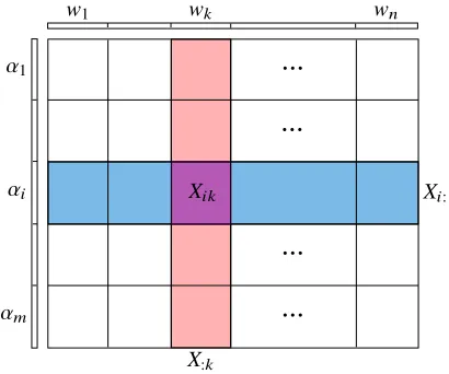
w1 wk wn

α₁

αi

αm

Xik Xi:

X:k

Figure 1: Partition of primal variablew, dual variableα, and the data matrixX.

whereP(w)is exactly the objective function in (1)1andg∗is the convex conjugate ofg. We assume

thatLhas a saddle point(w?, α?), that is,

L(w?, α) ≤ L(w?, α?) ≤ L(w, α?), ∀(w, α) ∈Rd×RN.

In this case, we havew?=arg min P(w)andα?=arg min D(α), andP(w?) = D(α?). The DSCOVR framework is based on solving the convex-concave saddle-point problem

min

w∈Rd _αmax_∈RN L(w, α). (8)

Since we assume thatghas a separable structure as in (2), we rewrite the saddle-point problem as

min w∈Rd _αmax_∈RN

1

m

m X

i=1 n X

k=1

αT

i Xikwk− 1

m

m X

i=1

f_i∗(αi)+ n X

k=1

gk(wk)

, (9)

where Xik ∈ RNi×dk for k = 1, . . . ,n are column partitions of Xi. For convenience, we define the following notations. First, let X = [X₁;. . .;Xm] ∈ RN×d be the overall data matrix, by stacking the Xi’s vertically. Conforming to the separation of g, we also partition X into block

columns X_:k ∈RN×dk for k = 1, . . . ,n, where eachX:k =[X1k;. . .;Xmk] (stacked vertically). For consistency, we also useXi:to denoteXifrom now on. See Figure 1 for an illustration.

We exploit the doubly separable structure in (9) by a doubly stochastic coordinate update algorithm outlined in Algorithm 1. Let p = {p₁, . . . ,pm} andq = {q1, . . . ,qn} be two probability distributions. During each iterationt, we randomly pick an indexj ∈ {1, . . . ,m}with probabilitypj,

and independently pick an indexl ∈ {1, . . . ,n} with probabilityql. Then we compute two vectors u(t_j+1) ∈ RNj and _v(t+1)

l ∈ R

dl (details to be discussed later), and use them to update the block

coordinates αj and wl while leaving other block coordinates unchanged. The update formulas in (10) and (11) use the proximal mappings of the (scaled) functions f∗_j andgl respectively. We

1. More technically, we need to assume that each fi is convex and lower semi-continuous so that f_i∗∗= fi(see, e.g.,

Algorithm 1DSCOVR framework

input: initial pointsw(0), α(0), and step sizesσifori=1, . . . ,mandτk fork =1, . . . ,n.

1: fort=0,1,2, . . . ,do

2: pick j ∈ {1, . . . ,m}andl ∈ {1, . . . ,n}randomly with distributionspandqrespectively. 3: computevariance-reducedstochastic gradientsu(t_j+1)andv_l(t+1).

4: update primal and dual block coordinates:

α(t+1)

i =

    

prox_σjf∗

j α

(t)

j +σju

(t+1) j

if

i= j, α(t)

i , ifi, j,

(10)

w_k(t+1) =    

prox_τ

lgl w

(t) l −τlv

(t+1) l

if

k =l,

w_k(t), ifk ,l. (11)

5: end for

recall that the proximal mapping for any convex functionφ:Rd→R∪ {∞}is defined as

prox_φ(v)=4arg min u∈Rd

(

φ(u)+ 1

2ku−vk2 )

.

There are several different ways to compute the vectorsu(t_j+1)andv_l(t+1)in Step 3 of Algorithm 1.

They should be the partial gradients or stochastic gradients of the bilinear coupling term inL(w, α) with respect toαjandwlrespectively. Let

K(w, α)=αTXw=

m X

i=1 n X

k=1

αT i Xikwk,

which is the bilinear term in L(w, α) without the factor 1/m. We can use the following partial gradients in Step 3:

¯

u(t_j+1)= ∂K(w

(t)_{, α}(t)₎

∂αj = n X

k=1

Xjkw_k(t),

¯

v_l(t+1)= 1 m

∂K(w(t), α(t))

∂wl = 1

m

m X

i=1

(Xil)Tα_i(t).

(12)

We note that the factor 1/mdoes not appear in the first equation because it multiplies bothK(w, α) and f_j∗(αj)in (9) and hence does not appear in updatingαj. Another choice is to use

u(t_j+1) = 1 ql

X_jlw_l(t),

v_l(t+1) = 1 pj

1

m(Xjl)

T_α(t) j ,

(13)

which are unbiased stochastic partial gradients, because

Elu(t_j+1) = n X

k=1

qk 1

qk

Xjkw_k(t) = n X

k=1

Xjkw_k(t) =u¯(t_j+1),

Ejv_l(t+1) = m X

i=1

pi1

pi 1

m(Xil)

T_α(t)

i =

1

m

m X

i=1

w₁ wn w₁ wn

α₁

α_m

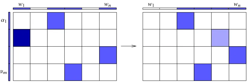
Figure 2: Simultaneous data and model parallelism. At any given time, each machine is busy updating one parameter block and its own dual variable. Whenever some machine is done, it is assigned to work on a random block that is not being updated.

whereEjandElare expectations with respect to the random indices jandlrespectively.

It can be shown that, Algorithm 1 converges to a saddle point ofL(w, α)with either choice (12) or (13) in Step 3, and with suitable step sizes σ_i andτk. It is expected that using the stochastic gradients in (13) leads to a slower convergence rate than applying (12). However, using (13) has the advantage of much less computation during each iteration. Specifically, it employs only one block matrix-vector multiplication for both updates, instead ofnandmblock multiplications done in (12).

More importantly, the choice in (13) is suitable for parallel and distributed computing. To see this, let(j(t),l(t))denote the pair of random indices drawn at iterationt(we omit the superscript(t) to simplify notation whenever there is no confusion from the context). Suppose for a sequence of consecutive iterationst, . . . ,t+s, there is no common index among j(t), . . . ,j(t+s), nor among l(t), . . . ,l(t+s), then theses+1 iterations can be done in parallel and they produce the same updates

as being done sequentially. Suppose there ares+1 processors or machines, then each can carry out

one iteration, which includes the updates in (13) as well as (10) and (11). These s+1 iterations

are independent of each other, and in fact can be done in any order, because each only involve one primal blockw_l(t) and one dual blockα_j(t), for both input and output (variables on the right and left

sides of the assignments respectively). In contrast, the input for the updates in (12) depend on all primal and dual blocks at the previous iteration, thus cannot be done in parallel.

In practice, suppose we havemmachines for solving problem (9), and each holds the data matrix Xi: in memory and maintains the dual blockαi, fori = 1, . . . ,m. We assume that the number of model partitionsnis larger thanm, and thenmodel blocks{w₁, . . . ,wn}are stored at one or more parameter servers. In the beginning, we can randomly pick m model blocks (sampling without

The idea of using doubly stochastic updates for distributed optimization in not new. It has been studied by Yun et al. (2014) for solving the matrix completion problem, and by Matsushima et al. (2014) for solving the saddle-point formulation of the ERM problem. Despite their nice features for parallelization, these algorithms inherit theO(1/√t)(orO(1/t) with strong convexity) sublinear convergence rate of the classical stochastic gradient method. They translate into high communication and computation cost for distributed optimization. In this paper, we propose new variants of doubly stochastic update algorithms by using variance-reduced stochastic gradients (Step 3 of Algorithm 1). More specifically, we borrow the variance-reduction techniques from SVRG (Johnson and Zhang, 2013) and SAGA (Defazio et al., 2014) to develop the DSCOVR algorithms, which enjoy fast linear rates of convergence. In the rest of this section, we summarize our theoretical results characterizing the three measures for DSCOVR: computation complexity, communication complexity, and synchronization cost. We compare them with distributed implementation of batch first-order algorithms.

2.1. Summary of Main Results

Throughout this paper, we usek · kto denote the standard Euclidean norm for vectors. For matrices, k · k denotes the operator (spectral) norm and k · kF denotes the Frobenius norm. We make the following assumption regarding the optimization problem (1).

Assumption 1 Each f_iis convex and differentiable, and its gradient is(1/γi)-Lipschitz continuous, i.e.,

k∇f_i(u)− ∇f_i(v)k ≤ 1 γi

ku−vk, ∀u,v ∈RNi, _i=1, . . . ,m. (14)

In addition, the regularization functiongisλ-strongly convex, i.e.,

g(w0) ≥g(w)+ξT(w0−w)+ λ

2kw0−wk2, ∀ξ ∈∂g(w), w0,w∈Rd.

Under Assumption 1, each f_i∗isγi-strongly convex (see, e.g., Hiriart-Urruty and Lemaréchal, 2001,

Theorem 4.2.2), andL(w, α)defined in (5) has a unique saddle point(w?, α?).

The condition (14) is often referred to as fibeing 1/γi-smooth. To simplify discussion, here we assumeγi = γ fori =1, . . . ,m. Under these assumptions, each composite function fi(Xiw)has a smoothness parameterkX_ik2/γ(upper bound on the largest eigenvalue of its Hessian). Their average

(1/m)Pm_i=1 fi(Xiw) has a smooth parameter kXk2/(mγ), which no larger than the average of the individual smooth parameters(1/m)Pm_i=1kXik2/γ. We define a condition number for problem (1) as the ratio between this smooth parameter and the convexity parameterλofg:

κ_bat= k_mλγXk2 ≤ 1 m

m X

i=1

kX_i:k2 λγ ≤

kXk_max2

λγ , (15)

where kXk_max = maxi{kX_i:k}. This condition number is a key factor to characterize the

iter-ation complexity of batch first-order methods for solving problem (1), i.e., minimizing P(w).

Specifically, to find a w such that P(w) − P(w?) ≤ , the proximal gradient method requires O (1+κ_bat)log(1/) iterations, and their accelerated variants require

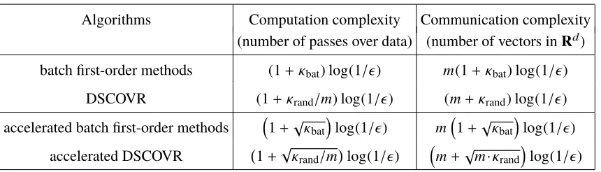
Algorithms Computation complexity Communication complexity (number of passes over data) (number of vectors inRd) batch first-order methods (1+κ_bat)log(1/) m(1+κ_bat)log(1/)

DSCOVR (1+κ_rand/m)log(1/) (m+κ_rand)log(1/)

accelerated batch first-order methods

1+√κ_bat

log(1/) m1+√κ_batlog(1/) accelerated DSCOVR 1+√κ_rand/mlog

(1/) m+√m·κ_randlog(1/) Table 1: Computation and communication complexities of batch first-order methods and DSCOVR

(for both SVRG and SAGA variants). We omit theO(·)notation in all entries and an extra log(1+κ_rand/m)factor for accelerated DSCOVR algorithms.

A fundamental baseline for evaluating any distributed optimization algorithms is the distributed implementation of batch first-order methods. Let’s consider solving problem (1) using the proximal gradient method. During every iteration t, each machine receives a copy of w(t) ∈ Rd from a master machine (through Broadcast), and computes the local gradientz_i(t)= X_iT∇fi(Xiw(t)) ∈Rd. Then a collective communication is invoked to compute the batch gradientz(t) =(1/m)Pm

i=1z (t)

i at

the master (Reduce). The master then takes a proximal gradient step, using z(t) and the proximal

mapping of g, to compute the next iterate w(t+1) and broadcast it to every machine for the next

iteration. We can also use the AllReduce operation in MPI to obtain z(t) at each machine without

a master. In either case, the total number of passes over the data is twice the number of iterations (due to matrix-vector multiplications using both Xi and X_iT), and the number of vectors in Rd sent/received across all machines is 2mtimes the number of iterations (see Table 1). Moreover, all

communications are collective and synchronous.

Since DSCOVR is a family of randomized algorithms for solving the saddle-point problem (8), we would like to find(w, α)such thatkw(t)−w?k2+(1/m)kα(t)−α?k2 ≤ holds in expectation

and with high probability. We list the communication and computation complexities of DSCOVR in Table 1, comparing them with batch first-order methods. Similar guarantees also hold for reducing the duality gapP(w(t))−D(α(t)), wherePandDare defined in (6) and (7) respectively.

The key quantity characterizing the complexities of DSCOVR is the condition number κ_rand, which can be defined in several different ways. If we pick the data blockiand model blockk with

uniform distribution, i.e.,p_i =1/mfori=1, . . . ,mandq_k =1/nfork =1, . . . ,n, then

κ_rand= nkXkm2×n

λγ , where kXkm×n=max

i,k kXikk. (16)

Comparing the definition ofκ_batin (15), we haveκ_bat ≤ κ_randbecause

1

mkXk 2 _≤ 1

m

m X

i=1

kXik2 ≤ 1

m

m X

i=1 n X

k=1

kXikk2 ≤nkXkm2×n.

WithXi: =[Xi1· · ·Xim]∈RNi×dandX:k =[X1k;. . .;Xmk]∈RN×dk, we can also define

κ0 rand =

kXk_max2 _,F

λγ , where kXkmax,F =max i,k

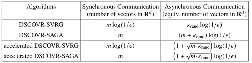
Algorithms Synchronous Communication Asynchronous Communication (number of vectors inRd) (equiv. number of vectors inRd)

DSCOVR-SVRG mlog(1/) κ_randlog(1/)

DSCOVR-SAGA m (m+κ_rand)log(1/)

accelerated DSCOVR-SVRG mlog(1/) 1+√m·κ_randlog(1/)

accelerated DSCOVR-SAGA m 1+√m·κ_randlog(1/)

Table 2: Breakdown of communication complexities into synchronous and asynchronous commu-nications for two different types of DSCOVR algorithms. We omit theO(·) notation and an extra log(1+κ_rand/m) factor for accelerated DSCOVR algorithms.

In this case, we also haveκ_bat≤ κ_rand0 becausekXk_max≤ kXk_max,F. Finally, if we pick the pair(i,k) with non-uniform distributionpi= kXi:k2_F/kXk_F2 andqk = kX:kk_F2/kXk2_F, then we can define

κ00 rand =

kXk2_F

mλγ . (18)

Again we haveκ_bat ≤ κ00_randbecausekXk ≤ kXk_F. We may replaceκ_randin Tables 1 and 2 by either κ0

randorκ00rand, depending on the probability distributionspandqand different proof techniques.

From Table 1, we observe similar type of speed-ups in computation complexity, as obtained by variance reduction techniques over the batch first-order algorithms for convex optimization (e.g., Le Roux et al., 2012; Johnson and Zhang, 2013; Defazio et al., 2014; Xiao and Zhang, 2014; Lan and Zhou, 2018; Allen-Zhu, 2017), as well as for convex-concave saddle-point problems (Zhang and Xiao, 2017; Balamurugan and Bach, 2016). Basically, DSCOVR algorithms have potential improvement over batch first-order methods by a factor ofm(for non-accelerated algorithms) or√m

(for accelerated algorithms), but with a worse condition number. In the worst case, the ratio between

κ_randandκ_batmay be of ordermor larger, thus canceling the potential improvements.

More interestingly, DSCOVR also has similar improvements in terms of communication com-plexity over batch first-order methods. In Table 2, we decompose the communication comcom-plexity of DSCOVR into synchronous and asynchronous communication. The decomposition turns out to be different depending on the variance reduction techniques employed: SVRG (Johnson and Zhang, 2013) versus SAGA (Defazio et al., 2014). We note that DSCOVR-SAGA essentially requires only asynchronous communication, because the synchronous communication ofmvectors are only

necessary for initialization with non-zero starting point.

The comparisons in Table 1 and 2 give us good understanding of the complexities of different algorithms. However, these complexities are not accurate measures of their performance in practice. For example, collective communication of m vectors in Rd can often be done in parallel over a spanning tree of the underlying communication network, thus only cost log(m)times (instead ofm

times) compared with sending only one vector. Also, for point-to-point communication, sending one vector inRdaltogether can be much faster than sendingnsmaller vectors of total lengthdseparately.

2.2. Related Work

There is an extensive literature on distributed optimization. Many algorithms developed for machine learning adopt the centralized communication setting, due to the wide availability of supporting standards and platforms such as MPI, MapReduce and Spark (as discussed in the introduction). They include parallel implementations of the batch first-order and second-order methods (e.g., Lin et al., 2014; Chen et al., 2014; Lee et al., 2017a), ADMM (Boyd et al., 2011), and distributed dual coordinate ascent (Yang, 2013; Jaggi et al., 2014; Ma et al., 2015).

For minimizing the average function(1/m)Pm

i=1 fi(w), in the centralized setting and with only first-order oracles (i.e., gradients of fi’s or their conjugates), it has been shown that distributed

implementation of accelerated gradient methods achieves the optimal convergence rate and commu-nication complexity (Arjevani and Shamir, 2015; Scaman et al., 2017). The problem (1) we consider has the extra structure of composition with a linear transformation by the local data, which allows us to exploit simultaneous data and model parallelism using randomized algorithms and obtain improved communication and computation complexity.

Most work on asynchronous distributed algorithms exploit model parallelism in order to reduce the synchronization cost, especially in the setting with parameter servers (e.g., Li et al., 2014; Xing et al., 2015; Aytekin et al., 2016). Besides, delay caused by the asynchrony can be incorporated to the step size to gain practical improvement on convergence (e.g., Agarwal and Duchi, 2011; McMahan and Streeter, 2014; Sra et al., 2016), though the theoretical sublinear rates remain. There are also many recent work on asynchronous parallel stochastic gradient and coordinate-descent algorithms for convex optimization (e.g., Recht et al., 2011; Liu et al., 2014; Shi et al., 2015; Reddi et al., 2015; Richtárik and Takáč, 2016; Peng et al., 2016). When the workloads or computing power of different machines or processors are nonuniform, they may significantly increaseiteration efficiency (number of iterations done in unit time), but often at the cost of requiring more iterations than their synchronous counterparts (due to delays and stale updates). So there is a subtle balance between iteration efficiency and iteration complexity (e.g., Hannah and Yin, 2017). Our discussions in Section 2.1 show that DSCOVR is capable of improving both aspects.

For solving bilinear saddle-point problems with a finite-sum structure, Zhang and Xiao (2017) proposed a randomized algorithm that works with dual coordinate update but full primal update. Yu et al. (2015) proposed a doubly stochastic algorithm that works with both primal and dual coordinate updates based on equation (12). Both of them achieved accelerated linear convergence rates, but neither can be readily applied to distributed computing. In addition, Balamurugan and Bach (2016) proposed stochastic variance-reduction methods (also based on SVRG and SAGA) for solving more general convex-concave saddle point problems. For the special case with bilinear coupling, they obtained similar computation complexity as DSCOVR. However, their methods require full model updates at each iteration (even though working with only one sub-block of data), thus are not suitable for distributed computing.

Algorithm 2DSCOVR-SVRG

input: initial points ¯w(0), ¯α(0), number of stagesSand number of iterations per stage M. 1: fors=0,1,2, . . . ,S−1do

2: u¯(s) = Xw¯(s) and ¯v(s) = _m1XTα¯(s) 3: w(0) =w¯(s) andα(0)= α¯(s)

4: fort=0,1,2, . . . ,M−1do

5: pick j∈ {1, . . . ,m}andl∈ {1, . . . ,n}randomly with distributionspandqrespectively.

6: compute variance-reduced stochastic gradients:

u(t_j+1) = u¯(s)_j + 1 ql

Xjl w_l(t)−w¯_l(s), (19)

v_l(t+1) = v¯_l(s)+ 1 pj

1

m(Xjl)

T _α(t) j −α¯

(s) j

. (20)

7: update primal and dual block coordinates:

α(t+1)

i =

    

prox_σjf∗

j α

(t)

j +σju

(t+1) j

if

i= j, α(t)

i , ifi, j,

w_k(t+1) =    

prox_τ

lgl w

(t) l −τlv

(t+1) l

if

k =l,

w_k(t), ifk ,l.

8: end for

9: w¯(s+1)=w(M)and ¯α(s+1) =α(M).

10: end for

output: w¯(S)and ¯α(S).

3. The DSCOVR-SVRG Algorithm

From this section to Section 6, we present several realizations of DSCOVR using different variance reduction techniques and acceleration schemes, and analyze their convergence properties. These algorithms are presented and analyzed as sequential randomized algorithms. We will discuss how to implement them for asynchronous distributed computing in Section 7.

Algorithm 2 is a DSCOVR algorithm that uses the technique of SVRG (Johnson and Zhang, 2013) for variance reduction. The iterations are divided into stages and each stage has a inner loop. Each stage is initialized by a pair of vectors ¯w(s) _{∈ R}d _{and ¯α}(s) _{∈ R}N_{, which come from either} initialization (ifs = 0) or the last iterate of the previous stage (ifs > 0). At the beginning of each

stage, we compute the batch gradients

¯

u(s) = ∂ ∂α¯(s)

(α¯(s))TXw¯(s) = Xw¯(s), v¯(s) = ∂ ∂w¯(s)

1

m(α¯

(s)₎T_Xw¯(s) !

= 1 mX

T_α¯(s)_.

The vectors ¯u(s)and ¯v(s)share the same partitions asα(t)andw(t), respectively. Inside each stages,

are unbiased. More specifically, taking expectation ofu(t_j+1)with respect to the random indexlgives

Elu(t_j+1) =u¯(s)_j + n X

k=1

qk 1

qk

Xjk w(t)_k −w¯_k(s)=u¯(s)_j +Xj:w(t)−Xj:w¯(s)= Xj:w(t),

and taking expectation ofv_l(t+1)with respect to the random index jgives

Ejv_l(t+1) =v¯_l(s)+ m X

i=1

pi 1

pi 1

m(Xil)

T _α(t) i −α¯

(s) i

= ¯

v_l(s)+ 1 m(X:l)

T

α(t)_−α¯(s)

= 1 m(X:l)

T_α(t)_.

In order to measure the distance of any pair of primal and dual variables to the saddle point, we define a weighted squared Euclidean norm onRd+N. Specifically, for any pair(w, α)wherew∈Rd andα=[α₁, . . . , αm]∈RN withαi ∈RNi, we define

Ω(w, α) = λkwk2+ 1 m

m X

i=1

γikαik2. (21)

Ifγi = γ for alli = 1, . . . ,m, thenΩ(w, α) = λkwk2+ _mγkαk2. We have the following theorem concerning the convergence rate of Algorithm 2.

Theorem 1 Suppose Assumption 1 holds, and let (w?, α?) be the unique saddle point ofL(w, α). LetΓbe a constant that satisfies

Γ ≥ max

i,k (1

pi 1+

9kXikk2 2qkλγi

!

, 1 qk 1+

9nkXikk2 2mpiλγi

! )

. (22)

In Algorithm 2, if we choose the step sizes as

σi = _2γ 1 i(piΓ−1)

, i=1, . . . ,m, (23)

τk = 1 2λ(qkΓ−1)

, k =1, . . . ,n, (24)

and the number of iterations during each stage satisfiesM ≥ log(3)Γ, then for anys >0,

EfΩ w¯(s)−w?,α¯(s)−α?g

≤ 2

3 !s

Ω w¯(0)−w?,α¯(0)−α?. (25) The proof of Theorem 1 is given in Appendix A. Here we discuss how to choose the parameterΓ to satisfy (22). For simplicity, we assumeγi=γ for alli=1, . . . ,m.

• If we letkXkm×n=maxi,k{kXikk}and sample with the uniform distribution across both rows and columns, i.e.,pi =1/mfori=1, . . . ,mandqk =1/nfork =1, . . . ,n, then we can set

Γ=max{m,n} 1+ 9nkXk 2

m×n 2λγ

!

=max{m,n} 1+ 9

2κrand !

,

whereκ_rand=nkXk_m2_×n

• An alternative condition forΓto satisfy is (shown in Section A.1 in the Appendix)

Γ ≥max

i,k

    

1

p_i* ,

1+ 9kX:kk2F 2q_kmλγ_i+

-, 1

q_k * ,

1+ 9kXi:k2F 2p_imλγ_i+

-    

. (26)

Again using uniform sampling, we can set

Γ=max{m,n}*

,

1+ 9kXkmax2 ,F

2λγ +

-=max{m,n} 1+ 9

2κ0rand

!

,

wherekXk_max,F =maxi,k{kXi:kF,kX:kkF}andκ_rand0 = kXk_max2 _,F(λγ)as defined in (17). • Using the condition (26), if we choose the probabilities to be proportional to the squared

Frobenius norms of the data partitions, i.e.,

pi=

kXi:k_F2

kXk2_F , qk =

kX_:kk2_F

kXk_F2 , (27)

then we can choose

Γ= 1

mini,k{pi,qk}

*

,

1+ 9kXk2F 2mλγ +

-= 1

mini,k{pi,qk} 1+ 9 2κ

00 rand

!

,

whereκ00

rand= kXkF2

(mλγ). Moreover, we can set the step sizes as (see Appendix A.1)

σi =

mλ

9kXk_F2, τk = mγi 9kXk2_F.

• For the ERM problem (3), we assume that each loss functionφj, for j = 1, . . . ,N, is 1/ν

-smooth. According to (4), the smooth parameter for each fi isγi = γ = (N/m)ν. LetRbe the largest Euclidean norm among all rows ofX (or we can normalize each row to have the

same normR), then we havekXk_F2 ≤ N R2and

κ00 rand=

kXk_F2 mλγ ≤

N R2 mλγ =

R2

λν. (28)

The upper bound R2/(λν) is a condition number used for characterizing the iteration com-plexity of many randomized algorithms for ERM (e.g., Shalev-Shwartz and Zhang, 2013; Le Roux et al., 2012; Johnson and Zhang, 2013; Defazio et al., 2014; Zhang and Xiao, 2017). In this case, using the non-uniform sampling in (27), we can set the step sizes to be

σi =

λ

9R2 m

N, τk = γ

9R2 m N =

ν

9R2. (29)

Next we estimate the overall computation complexity of DSCOVR-SVRG in order to achieve E_Ω

requires going through the whole data setX, whose computational cost is equivalent tom×ninner

iterations. Therefore, the overall complexity of Algorithm 2, measured by total number of inner iterations, is

O mn+Γlog Ω (0)

! !

.

To simplify discussion, we further assume m ≤ n, which is always the case for distributed

imple-mentation (see Figure 2 and Section 7). In this case, we can letΓ = n(1+ (9/2)κ_rand). Thus the above iteration complexity becomes

O n(1+m+κ_rand)log(1/). (30)

Since the iteration complexity in (30) counts the number of blocksX_ik being processed, the number

of passes over the whole datasetX can be obtained by dividing it bymn, i.e.,

O 1+ κrand m

log(1/)

. (31)

This is the computation complexity of DSCOVR listed in Table 1. We can replaceκ_randbyκ0 randor κ00

rand depending on different proof techniques and sampling probabilities as discussed above. We

will address the communication complexity for DSCOVR-SVRG, including its decomposition into synchronous and asynchronous ones, after describing its implementation details in Section 7.

In addition to convergence to the saddle point, our next result shows that the primal-dual optimality gap also enjoys the same convergence rate, under slightly different conditions.

Theorem 2 Suppose Assumption 1 holds, and letP(w)andD(α)be the primal and dual functions defined in(6)and(7), respectively. LetΛandΓbe two constants that satisfy

Λ ≥ kXikk2F, i=1, . . . ,m, k =1, . . . ,n, and

Γ ≥ max

i,k (1

pi 1+ 18Λ

qkλγi !

, 1 qk 1+

18nΛ

pimλγi ! )

.

In Algorithm 2, if we choose the step sizes as

σi = _γ 1 i(piΓ−1)

, i=1, . . . ,m, (32)

τk = _λ 1

(q_kΓ−1), k =1, . . . ,n, (33)

and the number of iterations during each stage satisfiesM ≥ log(3)Γ, then

EfP(w¯(s))−D(α¯(s))g ≤ 2

3 !s

2ΓP(w¯(0))−D(α¯(0)). (34)

The proof of Theorem 2 is given in Appendix B. In terms of iteration complexity or total number of passes to reachE

P(w¯(s))−D(α¯(s))

Algorithm 3DSCOVR-SAGA

input: initial pointsw(0), α(0), and number of iterationsM. 1: u¯(0) = Xw(0)and ¯v(0) = _m1XTα(0)

2: U_ik(0) = Xikw_k(0),V_ik(0) = _m1(α(_i0))TXik, for alli=1, . . . ,mandk =1, . . . ,K.

3: fort=0,1,2, . . . ,M−1do

4: pick j ∈ {1, . . . ,m}andl ∈ {1, . . . ,n}randomly with distributionspandqrespectively. 5: compute variance-reduced stochastic gradients:

u(t_j+1) = u¯(t)_j − 1 ql

U_jl(t)+ 1 ql

Xjlw_l(t), (35)

v_l(t+1) = v¯_l(t)− 1 pj

(V_jl(t))T + 1

pj 1

m(Xjl)

T_α(t)

j . (36)

6: update primal and dual block coordinates:

α(t+1)

i =

( _prox σjΦ∗_j α

(t)

j +σju

(t+1) j

if

i= j. α(t)

i , ifi, j,

w_k(t+1) =

( prox_τ

lgl w

(t) l −τlv

(t+1) l

if

k =l, w_k(t), ifi_, j.

7: update averaged stochastic gradients:

¯

u(t_i+1) =

_u¯(t)

j −U

(t)

jl +Xjlw (t)

l ifi= j,

¯

u(t)_i ifi, j,

¯

v_k(t+1) =

_v¯(t)

l −(V

(t) jl )

T ₊ 1

m(Xjl)Tα (t)

j ifk =l,

¯

v_k(t) ifk _,l,

8: update the table of historical stochastic gradients:

U_ik(t+1) =

_X

jlw_l(t) ifi= jandk =l,

U_ik(t) otherwise.

V_ik(t+1) =

1 m (Xjl)

T_α(t) j

T _if

i= jandk =l,

V_ik(t) otherwise.

9: end for

output: w(M)andα(M).

4. The DSCOVR-SAGA Algorithm

Algorithm 3 is a DSCOVR algorithm that uses the techniques of SAGA (Defazio et al., 2014) for variance reduction. This is a single stage algorithm with iterations indexed byt. In order to compute

the variance-reduced stochastic gradientsu(t_j+1)andv_l(t+1)at each iteration, we also need to maintain

The vector ¯u(t)shares the same partition asα(t) intomblocks, and ¯v(t)share the same partitions as w(t) intonblocks. The matrixU(t) is partitioned intom×nblocks, with each blockU_ik(t) ∈RNi×1.

The matrixV(t) is also partitioned intom×nblocks, with each blockV_ik(t) ∈R1×dk. According to

the updates in Steps 7 and 8 of Algorithm 3, we have

¯

u_i(t) =

n X

k=1

U_ik(t), i=1, . . . ,m, (37)

¯

v_k(t) =

m X

i=1

V_ik(t)T, k =1, . . . ,n. (38)

Based on the above constructions, we can show that u(t_j+1) is an unbiased stochastic gradient of

(α(t))TXw(t)with respect toαj, andv_l(t+1)is an unbiased stochastic gradient of(1/m) (α(t))TXw(t) with respect towl. More specifically, according to (35), we have

E_l

u(t_j+1) = ¯

u(t)_j −

n X

k=1

qk 1

qk

U_jk(t)

!

+

n X

k=1

qk 1

qk

Xjkw_k(t) !

= u¯(t)_j −

n X

k=1

U_jk(t)+

n X

k=1

X_jkw(t)_k

= u¯(t)_j −u¯(t)_j +Xj:w(t)

= Xj:w(t) =

∂ ∂αj

α(t)T

Xw(t), (39)

where the third equality is due to (37). Similarly, according to (36), we have

Ejv_l(t+1) = v¯_l(t)− m X

i=1

pi 1

pi (V_il(t))T

!

+

m X

i=1

pi 1

pim

(Xil)Tα(t)_i !

= v¯_l(t)−

m X

i=1

V_il(t)+ 1 m

m X

i=1

(Xil)Tα_i(t)

= v¯_l(t)−v¯_l(t)+ 1 m(X:l)

T_α(t)

= 1

m(X:l)

T_α(t) ₌ ∂

∂wl 1

m α

(t)T

Xw(t)

!

, (40)

where the third equality is due to (38). The following theorem is proved in Appendix C.

Theorem 3 Suppose Assumption 1 holds, and let (w?, α?) be the unique saddle point ofL(w, α). LetΓbe a constant that satisfies

Γ ≥ max

i,k (

1

pi 1+

9kXikk2 2qkλγi

!

, 1 qk 1+

9nkXikk2 2pimλγi !

, 1 piqk

)

. (41)

If we choose the step sizes as

σi = 1 2γi(piΓ−1)

, i=1, . . . ,m, (42)

τk = 1 2λ(qkΓ−1)

Algorithm 4Accelerated DSCOVR

input: initial points ˜w(0),α˜(0), and parameterδ >0.

1: forr =0,1,2, . . . ,do

2: find an approximate saddle point of (46) using one of the following two options:

• option 1: run Algorithm 2 withS= 2 log_log(2₍₃(1+_/2)δ)) andM =log(3)Γ_δ to obtain (w˜(r+1),α˜(r+1)) =DSCOVR-SVRG(w˜(r),α˜(r),S,M).

• option 2: run Algorithm 3 withM =6 log8(1+₃δ)Γ_δ to obtain (w˜(r+1),α˜(r+1)) =DSCOVR-SAGA(w˜(r),α˜(r),M).

3: end for

Then the iterations of Algorithm 3 satisfy, fort=1,2, . . .,

EfΩ w(t)−w?, α(t)−α?g

≤ 1− 1

3Γ !t ₄

3Ω w(0)−w?, α(0)−α?

. (44)

The condition on Γ in (41) is very similar to the one in (22), except that here we have an additional term 1/(p_iq_k) when taking the maximum overiandk. This results in an extramnterm

in estimatingΓunder uniform sampling. Assumingm≤ n(true for distributed implementation), we

can let

Γ= n 1+ 9

2κrand !

+mn.

According to (44), in order to achieveE_Ω

(w(t)− w?, α(t)− α?)

≤ , DSCOVR-SAGA needs

O Γlog(1/)iterations. Using the above expression for

Γ, the iteration complexity is

O n(1+m+κ_rand)log(1/), (45)

which is the same as (30) for DSCOVR-SVRG. This also leads to the same computational complexity measured by the number of passes over the whole dataset, which is given in (31). Again we can replace κ_rand by κ0

rand or κ00rand as discussed in Section 3. We will discuss the communication

complexity of DSCOVR-SAGA in Section 7, after describing its implementation details.

5. Accelerated DSCOVR Algorithms

In this section, we develop an accelerated DSCOVR algorithm by following the “catalyst” frame-work (Lin et al., 2015; Frostig et al., 2015). More specifically, we adopt the same procedure by Balamurugan and Bach (2016) for solving convex-concave saddle-point problems.

Let δ > 0 be a parameter which we will determine later. Consider the following perturbed saddle-point function for roundr:

L(r)_δ (w,a) =L(w, α)+ δλ

2 kw−w˜(r)k2−

δ

2m

m X

i=1

γikαi−α˜_i(r)k2. (46)

Under Assumption 1, the function L(r_δ)(w,a) is (1+ δ)λ-strongly convex in w and(1+δ)γi/m -strongly concave inαi. LetΓ_δ be a constant that satisfies

Γδ ≥ max

i,k (

1

pi 1+

9kX_ikk2

2qkλγi(1+δ)2 !

, 1 qk 1+

9nkX_ikk2

2pimλγi(1+δ)2 !

, 1 piqk

)

,

where the right-hand side is obtained from (41) by replacingλandγiwith(1+δ)λand(1+δ)γi respectively. The constant Γ_δ is used in Algorithm 4 to determine the number of inner iterations to run with each round, as well as for setting the step sizes. The following theorem is proved in Appendix D.

Theorem 4 Suppose Assumption 1 holds, and let (w?, α?) be the saddle-point of L(w, α). With either options in Algorithm 4, if we choose the step sizes (inside Algorithm 2 or Algorithm 3) as

σi = _2(1+δ 1

)γi(piΓδ−1)

, i=1, . . . ,m, (47)

τk = 1

2(1+δ)λ(q_kΓδ −1), k =1, . . . ,n. (48)

Then for allr ≥ 1,

EfΩ w˜(r)−w?,α˜(r)−α?g

≤ 1− 1

2(1+δ) !2r

Ω w˜(0)−w?,α˜(0)−α?. According to Theorem 4, in order to haveE_Ω ˜

w(r)−w?,α˜(r)−α? ≤ , we need the number

of roundsr to satisfy

r ≥ (1+δ)log

_Ω w˜(0)−w?,α˜(0)−α?

.

Following the discussions in Sections 3 and 4, when using uniform sampling and assumingm ≤ n,

we can have

Γ_δ =n 1+ 9κrand

2(1+δ)2 !

+mn. (49)

Then the total number of block coordinate updates in Algorithm 4 is

O (1+δ)Γ_δlog(1+δ)log(1/),

where the log(1+δ)factor comes from the number of stagesSin option 1 and number of stepsMin

option 2. We hide the log(1+δ)factor with theOHnotation and plug (49) into the expression above

to obtain

H

O n (1+δ)(1+m)+ κrand (1+δ)

! log 1

! !

.

• Ifκ_rand > 1+m, we can minimizing the above expression by choosingδ=

q κrand

1+m−1, so that the overall iteration complexity becomesOH

n√mκ_randlog(1/).

• Ifκ_rand ≤ m+1, then no acceleration is necessary and we can chooseδ=0 to proceed with a

single round. In this case, the iteration complexity isO(mn)as seen from (49).

Therefore, in either case, the total number of block iterations by Algorithm 4 can be written as

H

Omn+n√mκ_randlog(1/). (50)

As discussed before, the total number of passes over the whole dataset is obtained by dividing bymn:

H

O1+pκ_rand/mlog(1/).

This is the computational complexity of accelerated DSCOVR listed in Table 1.

5.1. Proximal Mapping for Accelerated DSCOVR

When applying Algorithm 2 or 3 to approximate the saddle-point of (46), we need to replace the proximal mappings ofgk(·)and f_i∗(·)by those ofgk(·)+(δλ/2)k · −w˜_k(r)k2and f_i∗(·)+(δγi/2)k ·

−α˜(r)_i k2, respectively. More precisely, we replacew_k(t+1)=prox_τ

kgk w

(t) k −τkv

(t+1) k

by

w_k(t+1) =arg min

wk∈Rdk

(

gk(wk)+

δλ

2 wk−w˜

(r)

k

2₊ 1

2τk

wk−

w_k(t)−τ_kv_k(t+1)

2)

=prox τk 1+τkδλgk

1 1+τkδλ

w(t)_k −τkv_k(t+1)

+ τkδλ 1+τkδλ ˜

w_k(r)

!

, (51)

and replaceα(t+1)

i =proxσif_i∗ α

(t)

i +σiu

(t+1) i

by

α(t+1)

i =arg min

αi∈RNi

(

f_i∗(αi)+

δγi

2

αi−α˜

(r)

i

2₊ 1

2σi

αi−

α(t)

i +σiu

(t+1) i

2)

=prox σi 1+σiδγif

∗

i

1 1+σiδγi

α(t)

i +σiu

(t+1) i

+ σiδγi 1+σiδγi˜

α(r) i

!

. (52)

We also examine the number of inner iterations determined byΓ_δ and how to set the step sizes. If we chooseδ=qκrand

1+m−1, thenΓδ in (49) becomes Γ_δ =n 1+ 9κrand

2(1+δ)2 !

+mn=n 1+ 9κrand

2κ_rand/(m+1) !

+mn=5.5(m+1)n.

Therefore a small constant number of passes is sufficient within each round. Using the uniform sampling, the step sizes can be estimated as follows:

σi= 1

2(1+δ)γi(piΓδ −1)

≈ 1

2√κ_rand/mγi(5.5n−1)

≈ 1

11γin

√

κ_rand/m, (53) τk = _2(1+δ 1

)λ(qkΓδ−1)

≈ 1

2√κ_rand/mλ(5.5m−1) ≈

1

11λ√m·κ_rand. (54)

6. Conjugate-Free DSCOVR Algorithms

A major disadvantage of primal-dual algorithms for solving problem (1) is the requirement of computing the proximal mapping of the conjugate function f_i∗, which may not admit closed-formed

solution or efficient computation. This is especially the case for logistic regression, one of the most popular loss functions used in classification.

Lan and Zhou (2018) developed “conjugate-free” variants of primal-dual algorithms that avoid computing the proximal mapping of the conjugate functions. The main idea is to replace the Euclidean distance in the dual proximal mapping with a Bregman divergence defined over the conjugate function itself. This technique has been used by Wang and Xiao (2017) to solve structured ERM problems with primal-dual first order methods. Here we use this approach to derive conjugate-free DSCOVR algorithms. In particular, we replace the proximal mapping for the dual update

α(t+1)

i =proxσif_i∗ α

(t)

i +σiu

(t+1) i

=arg min αi∈Rni

(

f_i∗(αi)−α

i, u_i(t+1)+ 1 2σi

αi−α

(t)

i

2)

,

by

α(t+1)

i =arg min

αi∈Rni

(

f_i∗(αi)−αi, u_i(t+1)+ _σ1 i

B_i α_i, α_i(t) )

, (55)

whereB_i(αi, α_i(t))= f_i∗(αi)−∇f_i∗(α_i(t)), αi−α(t)_i .The solution to (55) is given by

α(t+1)

i =∇fi β

(t+1) i

,

where β(t+1)

i can be computed recursively by

β(t+1)

i =

β(t)

i +σiu

(t+1) i 1+σi

, t ≥0,

with initial condition β(0)

i = ∇f

∗

i(α (0)

i ) (see Lan and Zhou, 2018, Lemma 1). Therefore, in order to update the dual variablesαi, we do not need to compute the proximal mapping for the conjugate function f_i∗; instead, taking the gradient of fi at some easy-to-compute points is sufficient. This conjugate-free update can be applied in Algorithms 1, 2 and 3.

For the accelerated DSCOVR algorithms, we replace (52) by

α(t+1)

i =arg min

αi∈Rni

(

f_i∗(αi)−αi,u(t_i+1)+ _σ1 i

B_i α_i, α(t)_i +δγ

B_i α_i,α˜(t_i+1) )

.

The solution to the above minimization problem can also be written as

α(t+1)

i =∇fi β

(t+1) i

,

where β(t+1)

i can be computed recursively as

β(t+1)

i =

β(t)

t +σiu_i(t+1)+σiδγβ˜i 1+σi+σiδγ

, t ≥0,

with the initialization β(0)

i =∇f

∗

i α

(0) i

and ˜β

i=∇f_i∗ α˜(r_i ).

00 00 11 11 00 00 11 11

00 00 11 11

0 0 1 1 0 0 1 1 00 00 11 11 00

11 00

1101 001100110011

scheduler

server 1 server j serverh

worker 1 workeri workerm

1

1

2

2

3 3

¯

w(s)

• resetsSfree={1, . . . ,n} • sends “sync” message to

all servers and workers at beginning of each stage

w(t)

k, k∈ S1 w

(t)

k, k∈ Sj w

(t)

k, k∈ Sh

X1:, ¯u(

s)

1

¯ α(s)

1 ,α

(t)

1

¯

w(s), ¯v(s)

Xi:, ¯u(

s)

i

¯ α(s)

i ,α

(t)

i

¯

w(s), ¯v(s)

Xm:, ¯u(ms) ¯ α_m(s),α_m(t)

¯

w(s), ¯v(s)

Figure 3: A distributed system for implementing DSCOVR consists of m workers, h parameter

servers, and one scheduler. The arrows labeled with the numbers 1, 2 and 3 represent three collective communications at the beginning of each stage in DSCOVR-SVRG.

7. Asynchronous Distributed Implementation

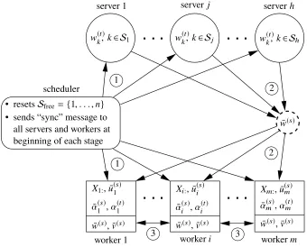
In this section, we show how to implement the DSCOVR algorithms presented in Sections 3–6 in a distributed computing system. We assume that the system provide both synchronous collective communication and asynchronous point-to-point communication, which are all supported by the MPI standard (MPI Forum, 2012). Throughout this section, we assumem< n(see Figure 2).

7.1. Implementation of DSCOVR-SVRG

In order to implement Algorithm 2, the distributed system need to have the following components (see Figure 3):

• mworkers. Each workeri, fori=1, . . . ,m, stores the following local data and variables :

– data matrixXi: ∈RNi×d. – vectors inRNi: ¯_u(s)

i ,α

(t) i , ¯α

(s)

i .

– vectors inRd: ¯w(s), ¯v(s).

• hparameter servers. Each serverjstores a subset of the blocks

w_k(t) ∈Rdk :_{k ∈ S}

j , where

S₁, . . . ,Shform a partition of the set{1, . . . ,n}.

• one scheduler. It maintains a set of block indicesS_free ⊆ {1, . . . ,n}. At any given time,S_free

contains indices of parameter blocks that are not currently updated by any worker.

The reason for having h > 1 servers is not about insufficient storage for parameters, but rather to

avoid the communication overload between only one server and allmworkers (mcan be in hundreds).

At the beginning of each stages, the following three collective communications take place across

the system (illustrated in Figure 3 by arrows with circled labels 1, 2 and 3):

(1) The scheduler sends a “sync” message to all servers and workers, and resetsS_free={1, . . . ,n}.

(2) Upon receiving the “sync” message, the servers aggregate their blocks of parameters together to form ¯w(s)and send it to all workers (e.g., through the AllReduce operation in MPI).

(3) Upon receiving ¯w(s), each worker compute ¯u_i(s) = Xi:w¯(s) and (Xi:)Tα¯(s)_i , then invoke a collective communication (AllReduce) to compute ¯v(s) =(1/m)Pm_i=1(Xi:)Tα¯(s)_i .

The number of vectors in Rd sent and received during the above process is 2m, counting the

communications to form ¯w(s) and ¯v(s) atmworkers (ignoring the short “sync” messages).

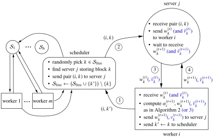
After the collective communications at the beginning of each stage, all workers start working on the inner iterations of Algorithm 2 in parallel in an asynchronous, event-driven manner. Each worker interacts with the scheduler and the servers in a four-step loop shown in Figure 4. There are alwaysmiterations taking place concurrently (see also Figure 2), each may at a different phase of

the four-step loop:

(1) Whenever workerifinishes updating a block k0, it sends the pair (i,k0) to the scheduler to request for another block to update. At the beginning of each stage,k0is not needed.

(2) When the scheduler receives the pair(i,k0), it randomly choose a blockkfrom the list of free

blocksS_free(which are not currently updated by any worker), looks up for the serverjwhich

stores the parameter block w_k(t) (i.e., Sj 3 k), and then send the pair (i,k) to server j. In addition, the scheduler updates the listS_freeby addingk0and deleting k.

(3) When server j receives the pair (i,k), it sends the vector w(t)_k to worker i, and waits for

receiving the updated versionw_k(t+1)from workeri.

(4) After worker i receives w_k(t), it computes the updates α(t)_i and w_k(t) following steps 6-7 in

Algorithm 2, and then sendw_k(t+1)back to server j. At last, it assigns the value ofktok0and

send the pair(i,k0) to the scheduler, requesting the next block to work on.

The amount of point-to-point communication required during the above process is 2d_kfloat numbers,

for sending and receivingw_k(t) andw_k(t+1) (we ignore the small messages for sending and receiving

(i,k0) and (i,k)). Since the blocks are picked randomly, the average amount of communication

per iteration is 2d/n, or equivalent to 2/n vectors inRd. According to Theorem 1, each stage of Algorithm 2 requires log(3)Γinner iterations; In addition, the discussions above (30) show that we can take Γ = n(1+(9/2)κ_rand). Therefore, the average amount of point-to-point communication

...

...

scheduler

server j

workeri

worker 1 workerm

S1 Sh

(i,k′) (i,k)

w(

t₎ k (,v¯

(t₎

k ) w

(t₊1) k (,v¯

(t₊₁₎

k )

1 2

3 4

• randomly pickk ∈ Sfree • find serverjstoring blockk

• send pair(i,k)to server j

• Sfree ← Sfree∪ {k′}\ {k}

• receivew(

t₎

k (and ¯v

(t₎ k )

• computeα_i(t+1),w(t+1)

k (,v¯ (t₊1)

k )

as in Algorithm 2(or 3)

• sendw(

t₊1) k (,v

(t₊₁₎

k )to server j

• sendk′←k to scheduler • receive pair(i,k)

• sendw(

t)

k (and ¯v

(t) k )

to workeri

• wait to receive

w(

t₊1)

k (and ¯v

(t₊₁₎

k )

Figure 4: Communication and computation processes for one inner iteration of DSCOVR-SVRG (Algorithm 2). The blue texts in the parentheses are the additional vectors required by DSCOVR-SAGA (Algorithm 3). There are always miterations taking place in parallel

asynchronously, each evolving around one worker. A server may support multiple (or zero) iterations if more than one (or none) of its stored parameter blocks are being updated.

Now we are ready to quantify the communication complexity of DSCOVR-SVRG to find an

-optimal solution. Our discussions above show that each stage requires collective communication of 2m vectors inRd and asynchronous point-to-point communication of equivalently κ_rand such vectors. Since there are totalO(log(1/))stages, the total communication complexity is

O (m+κ_rand)log(1/).

This gives the communication complexity shown in Table 1, as well as its decomposition in Table 2.

7.2. Implementation of DSCOVR-SAGA

We can implement Algorithm 3 using the same distributed system shown in Figure 3, but with some modifications described below. First, the storage at different components are different:

• mworkers. Each workeri, fori=1, . . . ,m, stores the following data and variables:

– data matrixX_i: ∈RNi×d

– vectors inRNi: α(t)

i ,u (t) i , ¯u

(t) i , andU

(t)

– vector inRd: V_i(t)_: =

V_i(t)₁ · · ·V_in(t)T (which is the

ith row ofV(t), withV_ik(t) ∈R1×dk).

– buffers for communication and update ofw_k(t) and ¯v_k(t)(both stored at some server).

• hservers. Each server jstores a subset of blocks

w(t)_k, v¯_k(t) ∈Rdk :_{k ∈ S}

j , for j=1, . . . ,n. • one scheduler. It maintains the set of indicesS_free ⊆ {1, . . . ,n}, same as in DSCOVR-SVRG.

Unlike DSCOVR-SVRG, there is no stage-wise “sync” messages. All workers and servers work in parallel asynchronously all the time, following the four-step loops illustrated in Figure 4 (including blue colored texts in the parentheses). Within each iteration, the main difference from DSCOVR-SVRG is that, the server and worker need to exchange two vectors of lengthdk: w_k(t) andv_k(t) and

their updates. This doubles the amount of point-to-point communication, and the average amount of communication per iteration is 4/nvectors of lengthd. Using the iteration complexity in (45),

the total amount of communication required (measured by number of vectors of lengthd) is

O (m+κ_rand)log(1/),

which is the same as for DSCOVR-SVRG. However, its decomposition into synchronous and asyn-chronous communication is different, as shown in Table 2. If the initial vectorsw(0) ,0 orα(0) ,0,

then one round of collective communication is required to propagate the initial conditions to all servers and workers, which reflect theO(m)synchronous communication in Table 2.

7.3. Implementation of Accelerated DSCOVR

Implementation of the accelerated DSCOVR algorithm is very similar to the non-accelerated ones. The main differences lie in the two proximal mappings presented in Section 5.1. In particular, the primal update in (51) needs the extra variable ˜w_k(r), which should be stored at a parameter server

together withw_k(t). We modify the four-step loops shown in Figures 4 as follows:

• Each parameter server j stores the extra block parameters ˜

w_k(r),k ∈ S_j . During step (3),

˜

w_k(r)is send together withw_k(t)(for SVRG) or(w_k(t),v_k(t))(for SAGA) to a worker.

• In step (4), no update of ˜w_k(r)is sent back to the server. Instead, whenever switching rounds,

the scheduler will inform each server to update their ˜w_k(r)to the most recentw_k(t).

For the dual proximal mapping in (52), each workerineeds to store an extra vector ˜α(r_i ), and reset it to

the most recentα(t)

i when moving to the next round. There is no need for additional synchronization or collective communication when switching rounds in Algorithm 4. The communication complexity (measured by the number of vectors of lengthd sent or received) can be obtained by dividing the

iteration complexity in (50) byn, i.e.,O (m+√mκ_rand)log(1/), as shown in Table 1.

Finally, in order to implement the conjugate-free DSCOVR algorithms described in Section 6, each workerisimply need to maintain and update an extra vector β_i(t)locally.

8. Experiments

CPU #cores RAM network operating system

dual Intel®_Xeon®_{processors 16 128 GB 10 Gbps Windows}®_Server

E5-2650 (v2), 2.6 GHz 1.8 GHz Ethernet adapter (version 2012)

Table 3: Configuration of each machine in the distributed computing system.

algorithms presented in this paper, including the SVRG and SAGA versions, their accelerated variants, as well as the conjugate-free algorithms. All implementations are written in C++, using MPI for both collective and point-to-point communications (see Figures 3 and 4 respectively). On each worker machine, we also use OpenMP (OpenMP Architecture Review Board, 2011) to exploit the multi-core architecture for parallel computing, including sparse matrix-vector multiplications and vectorized function evaluations.

Implementing the DSCOVR algorithms requiresm+h+1 machines, among themmare workers

with local datasets, h are parameter servers, and one is a scheduler (see Figure 3). We focus on

solving the ERM problem (3), where the total of N training examples are evenly partitioned and

stored atmworkers. We partition thed-dimensional parameters intonsubsets of roughly the same

size (differ at most by one), where each subset consists of randomly chosen coordinates (without replacement). Then we store thensubsets of parameters onhservers, each getting either bn/hcor dn/hesubsets. As described in Section 7, we make the configurations to satisfyn>m> h ≥1.

For DSCOVR-SVRG and DSCOVR-SAGA, the step sizes in (29) are very conservative. In the experiments, we replace the coefficient 1/9 by two tuning parameter η_d and η_p for the dual and primal step sizes respectively, i.e.,

σi =ηd

λ R2 ·

m

N, τk =ηp ν

R2. (56)

For the accelerated DSCOVR algorithms, we useκ_rand= R2/(λν) as shown in (28) for ERM. Then the step sizes in (53) and (54), withγi = (m/N)νand a generic constant coefficientη, become

σi=

η_d nR

r

mλ ν ·

m

N, τk = η_p

R

r

ν

mλ. (57)

For comparison, we also implemented the following first-order methods for solving problem 1: • PGD: parallel implementation of the Proximal Gradient Descent method (using synchronous

collective communication over m machines). We use the adaptive line search procedure

proposed in Nesterov (2013), and the exact form used is Algorithm 2 in Lin and Xiao (2015). • APG: parallel implementation of the Accelerated Proximal Gradient method (Nesterov, 2004, 2013). We use a similar adaptive line search scheme to the one for PGD, and the exact form used (with strong convexity) is Algorithm 4 in Lin and Xiao (2015).

• ADMM: the Alternating Direction Method of Multipliers. We use the regularized consensus version in Boyd et al. (2011, Section 7.1.1). For solving the local optimization problems at each node, we use the SDCA method (Shalev-Shwartz and Zhang, 2013).

Dataset #instances (N) #features (d) #nonzeros

rcv1-train 677,399 47,236 49,556,258

webspam 350,000 16,609,143 1,304,697,446

splice-site 50,000,000 11,725,480 166,167,381,622

Table 4: Statistics of three datasets. Each feature vector is normalized to have unit norm.

These four algorithms all require mworkers only. Specifically, we use the AllReduce call in MPI

for the collective communications so that a separate master machine is not necessary.

We conducted experiments on three binary classification datasets obtained from the collection maintained by Fan and Lin (2011). Table 4 lists their sizes and dimensions. In our experiments, we used two configurations: one withm=20 andh=10 for two relatively small datasets,rcv1-train andwebspam, and the other withm=100 andh=20 for the large datasetsplice-site.

Forrcv1-train, we solve the ERM problem (3) with a smoothed hinge loss defined as

φj(t) =

      

0 ifyjt≥ 1,

1

2−yjt ifyjt≤ 0,

1

2(1−yjt)2 otherwise,

and φ∗

j(β)= (

yjβ+ 1₂β2 if −1≤ yjβ ≤ 0,

+∞ otherwise.

for j = 1, . . . ,N. This loss function is 1-smooth, thereforeν = 1; see discussion above (28). We

use the`₂ regularization g(w) = (λ/2)kwk2. Figures 5 and 6 show the reduction of the primal

objective gapP(w(t))−P(w?)by different algorithms, with regularization parameterλ=10−4and

λ = 10−6_{respectively. All started from the zero initial point. Here the N examples are randomly}

shuffled and then divided intomsubsets. The labels SVRG and SAGA mean DSCOVR-SVRG and

DSCOVR-SAGA, respectively, and A-SVRG and A-SAGA are their accelerated versions.

Since PGD and APG both use adaptive line search, there is no parameter to tune. For ADMM, we manually tuned the penalty parameter ρ(see Boyd et al., 2011, Section 7.1.1) to obtain good performance: ρ = 10−5 _{in Figure 5 and ρ = 10}−6 _{in Figure 6. For CoCoA+, two passes over}

the local datasets using a randomized coordinate descent method are sufficient for solving the local optimization problem (more passes do not give meaningful improvement). For DSCOVR-SVRG and SAGA, we usedη_p=η_d=20 to set the step sizes in (56). For DSCOVR-SVRG, each stage goes through the whole dataset 10 times, i.e., the number of inner iterations in Algorithm 2 isM=10mn.

For the accelerated DSCOVR algorithms, better performance are obtained with small periods to update the proximal points and we set it to be every 0.2 passes over the dataset, i.e., 0.2mninner

iterations. For accelerated DSCOVR-SVRG, we set the stage period (for variance reduction) to be

M= mn, which is actually longer than the period for updating the proximal points.

From Figures 5 and 6, we observe that the two distributed algorithms based on model averaging, ADMM and CoCoA+, converges relatively fast in the beginning but becomes very slow in the later stage. Other algorithms demonstrate more consistent linear convergence rates. Forλ = 10−4_{, the}

DSCOVR algorithms are very competitive compared with other algorithms. For λ = 10−6_{, the}

non-accelerated DSCOVR algorithms become very slow, even after tuning the step sizes. But the accelerated DSCOVR algorithms are superior in terms of both number of passes over data and wall-clock time (with adjusted step size coefficientη_p=10 andη_d=40).