Efficiently Reasoning with Interval Constraints in Forward Search Planning

(1)

The Thirty-Third AAAI Conference on Artificial Intelligence (AAAI-19)

Efficiently Reasoning with Interval Constraints in Forward Search Planning

Amanda Coles,

∗

Andrew Coles,

∗

Moises Martinez,

∗

Emre Savas,

∗

Juan Manuel Delfa,

∗∗

Tom´as de la Rosa,

†

Yolanda E-Mart´ın,

†

Angel Garc´ıa-Olaya

† ∗_{Department of Informatics, King’s College London [email protected]}

∗∗_{European Space Agency, Oxford, UK [email protected]}

†_{Department of Computer Science, Universidad Carlos III de Madrid}_{_{trosa,yescuder,agolaya}_}_@inf.uc3m.es

Abstract

In this paper we present techniques for reasoning natively with quantitative/qualitative interval constraints in state-based PDDLplanners. While these are considered important in modeling and solving problems in timeline based plan-ners; reasoning with these in PDDL planners has seen rel-atively little attention, yet is a crucial step towards making PDDL planners applicable in real-world scenarios, such as space missions. Our main contribution is to extend the plan-ner OPTICto reason natively with Allen interval constraints. We show that our approach outperforms bothMTP, the only PDDL planner capable of handling similar constraints and a compilation to PDDL2.1, by an order of magnitude. We go on to present initial results indicating that our approach is com-petitive with a timeline based planner on a Mars rover do-main, showing the potential of PDDLplanners in this setting.

1 Introduction

Interval constraints are fundamental to modeling real-world planning problems, allowing specification of constraints on the temporal relationships between the execution of actions and the achievement of facts. For example, a Mars Rover must take a pictureduringa period in which the rover is sta-tionary at the location, and remains so for some specified time before and after the image is taken. Such constraints appear frequently in applications, not only in space-based domains, but also in terrestrial scenarios from scheduling ac-tivities of nursing home assistance robots (Tran et al. 2017) to planning ocean liner repositioning (Tierney et al. 2012).

Due to their ubiquity in applications, reasoning with in-terval constraints has been a major focus of research in timeline-based planning systems (Cesta et al. 2012; Frank and Jonsson 2003; Chien et al. 2000). The need for expres-sive languages has been noted (Cushing et al. 2007), but handling such constraints in PDDL planners has seen rela-tively little attention. This paper is the first to bridge the gap between the two major paradigms in temporal planning, combining their strengths: the expressive temporal reason-ing of timeline planners and the powerful heuristics of PDDL state-based planners, that are not readily accessible to time-line planners, which typically use less-scalable partial-order planning approaches. This provides a new, more efficient

approach for reasoning with these problems; and paves the way for the use of decades of research on PDDLplanning in space applications typically dominated by timeline planners. The lack of attention to explicitly reasoning with interval constraints in PDDLhas been, in part, due to the fact that previous work noted they can be represented in PDDL2.1 by adding additional actions to the domain (Fox, Long, and Halsey 2004; Smith, Frank, and Cushing 2008). Early crit-ics argued that this type of approach is cumbersome, forcing a planner to do additional work (Smith 2003); and indeed, as the first to fully define, and empirically evaluate the per-formance of, such a compilation in this paper, we find its scalability is very poor.

Our main contribution is a novel approach for reasoning directly with interval constraints in state-based PDDL plan-ning. We extend PDDLto provide new mechanisms for rep-resenting interval constraints explicitly, and then go on to show how an expressive PDDLplanner, OPTIC, can be ex-tended to reason directly with these constraints. We evalu-ate the performance of our new approach against that of a compilation on a range of benchmark domains with inter-val constraints, showing empirically that it outperforms this compilation by an order of magnitude (sometimes several). Finally, to illustrate the potential of our work to in space applications, typically dominated by timeline planners, we provide an initial comparison to an APSItimeline planning system (Cesta et al. 2012), on an existing ESA Mars rover domain, originally written in DDL: the representation lan-guage for APSI. We observe that our planner performs better than APSIon many of the problem instances.

2 Background

2.1 PDDL Temporal Planning Problems

(2)

Constraint Satisfiediff

synchronize g{after [lb,ub] f} ∀j·change(j, g),∃i: 0≤i≤j·change(i,¬f)∧lb≤tj−ti≤ub

synchronize f{before [lb,ub] g} ∀i·change(i,¬f),∃j:j≥i·change(j, g)∧lb≤tj−ti≤ub

synchronize f{overlaps [lb,ub] g} ∀j·change(j,¬f),∃i: 0≤i≤j·cholds(i, j, g)

∧(lb≤tj−ti≤ub)

synchronize f{during [sl,su] [el,eu] g} ∀j, k·choldsc(j, k, f),∃i: 0≤i≤j· ∃l:l≥k·choldsc(i, l, g)

(whereeu <∞) ∧(sl≤tj−ti≤su)∧(el≤tl−tk≤eu)

synchronize f{during [sl,su] [el,∞] g} ∀j, k·choldsc(j, k, f),∃i: 0≤i≤j·

(cholds(i, n, g)∧(sl≤tj−ti≤su))

synchronize g{contains [sl,su] [el,eu] f} (∀i, l·choldsc(i, l, g),∃j:i≤j≤l· ∃k:j≤k≤l·

(whereeu <∞) choldsc(j, k, f)∧(sl≤tj−ti≤su)∧(el≤tl−tk≤eu))

synchronize g{contains [sl,su] [el,∞] f} (∀i·cholds(i, n, g),∃j:i≤j≤n· ∃k:j≤k≤n·

choldsc(j, k, f)∧(sl≤tj−ti≤su)

Table 1: Interval Constraint Semantics, w.r.t. a state trajectoryh(S0,0),(S1, t1), ...,(Sn, tn)iinduced by snap-actions[ai..an].

The conversion of each interval cosntraint to orderings on interval start (`) and end (a) points is shown below it in brackets.

must hold at its start, throughout its execution (invariants), and at its end, respectively. Instantaneous effects can oc-cur at the start or end ofA: eff+_`A(eff−_`A) denote proposi-tions added (resp. deleted) at the start; effnum_` Adenotes any numeric effects. Similarly, eff+_aA, eff−_a and effnum_a record effects at the end. All numerical effects are of the form

v{+=,-=,=}w.v+c(v∈v). The values of effects become available small amount of time,, after they occur.

Finally, each actionA has a duration constraint: a con-junction of numeric constraints applied to a special variable durAdenoting its duration. As a special case,instantaneous

actions have duration , and only one set of preconditions preAand effects eff+A, eff−A, and effnumA. A durative actionA can be split into two instantaneoussnap-actions,

A` and Aa, representing the start and end of A respec-tively.A`has precondition pre`Aand effects eff

+

`A, eff − `A, effnum_` A.Aais the analogous action for the end ofA.

A solution is a sequence of timestamped actions, with as-sociated durations, that transforms the initial stateI into a state that satisfiesG; such that the start and end precondi-tions of all acprecondi-tions are satisfied at the time they start/end; all invariant conditions hold throughout the duration of each action, and all temporal/duration constraints are respected.

2.2 Temporal Timeline-Based Planning

While timeline planners diverge in a number of ways they share common concepts, and their divergence is not crucial to the content of this paper. As we are working on a project related to the European Space Agency we use, without loss of generality, their APSI nomenclature and an APSI planner. A timeline planning task comprises a domain and prob-lem. The domain contains a set of componentsCand syn-chronizationsS among them. There are two main types of component: state variables, that model discrete subsystems (e.g. a camera) described by a set of statesV and transi-tions among them; and (typically bounded) numeric vari-ables, used to represent resources (e.g. memory). A timeline is a set of non-overlapping temporal intervals with associ-ated values of one single component. The timeline must be complete, i.e. it must define the valuevi ∈V of the

com-Figure 1: (a)bove: Example Synchronize Block in DDL; (b)elow: Example of temporal relation between goals

ponentci ∈ Cat any given timet ∈ [o, h], where[o, h]is

the interval of the problem defined by its origin and horizon. Components and timelines have no equivalent representa-tion in PDDL, but it is possible to post-process a PDDLplan to generate a timeline plan (Ocon et al. 2017).

Fundamental to timeline planning is the notion of a time intervalT, represented as two timepointshTs,Teidenoting

its start and end. A constraint between two intervalsXand

Y relates the start or end of X with the start or end ofY. A synchronizationsover a valueviis used to define the set

of interval constraints that must be satisfied in order to add

vi to the plan. For example, in Figure 1(a) three temporal

constraints are defined: during the time the picture is taken, the rover must stay in position; during the time the picture is taken, the platine (camera mast) must be pointing at the tar-get; and the time at which the rover is in position, must con-tain the time during which the platine is pointing at the tar-get. Note the synchronization over the valuevionly applies

when that value holds: in our example, for the camera to take the value TakingPicture(...) the conditions on the rover and platine must be satisfied; but, we are otherwise free to move the rover or platine without taking a picture. Synchroniza-tions are the analog of (pre)condiSynchroniza-tions and effects of PDDL actions, but with a richer temporal vocabulary.

(3)

com-munication window). The goals define a list of values for different timelines to be satisfied at some point within[o, h]. It is possible to define an interval in the plan at which each goal must be true and to define temporal relations over the goals, providing a partial order between them, as shown in Figure 1(b): as the plan must satisfy the goals these relations must be satisfied at least once in any valid plan.

Two intervals X and Y can be related in 13 possi-ble ways: 7 cases plus their inverses (equals has no inverse). Timeline planners such as APSI (Cesta et al. 2012), Europa (Frank and Jonsson 2003) and AS-PEN (Chien et al. 2000) provide a variety of qualitative (A EQUALS/MEETS/STARTS/ENDS B) and quantitative tempo-ral relations (e.g A BEFORE [lb,ub] B) between actions and/or states, thus effectively combining Allen’s interval algebra (Allen 1983) and quantitative temporal expres-sions (Dechter, Meiri, and Pearl 1991). A quantitative re-lation betweenXandY generalizes qualitative relations by limiting the lower bound (lb)/upper bound (ub) distance be-tween their endpoints. In this work we support all 13 Allen constraints, for brevity we focus on the quantitative straints listed in Table 1; the reasoning for qualitative con-straints can trivially be derived by settingub/lb/sl/su= 0

or∞as appropriate in the equivalent quantitative constraint. As the first step of translating a DDLmodel to PDDLwe introduce the notion of a ‘state holding’ durative action. This represents the transition of a DDLcomponentcjto, and then

from, a valuevi ∈V. For each componentcj that can take

value vi we create an action A, with associated fact cjvi,

that regulates the transition ofcjvi from false, to true, and

back again: preA`={¬cjvi}, eff+A`={cjvi}, pre_↔A= {cjvi}, eff−Aa={cjvi}. The challenge remains to enforce

temporal constraints between state-holding durative actions for differentDDLcomponents with respect to each other to respect the DDLsynchronization constraints (S). This redu-ces to enforcing interval constraints between starts and ends of PDDLdurative actions, the topic of the rest of the paper.

2.3 Interval Constraints vs PDDL3 Constraints

The ability to express constraints and preferences over the trajectory of the plan was introduced in PDDL3 (Gerevini et al. 2009) and a number of planners were developed to sup-port these (Benton, Coles, and Coles 2012; Edelkamp, Jab-bar, and Nazih 2006; Baier, Bachus, and McIlraith 2007). Two major semantic differences make PDDL 3 constraints insufficient to capture Allen constraints. The first is change semantics: DDLconstraints are defined w.r.t. steps at which the truth value of a fact (or formula) changes; whereas PDDL3 constraints are defined w.r.t. whether the truth value of a fact (or formula) holds at a step. Consider the DDL constraintsynchronize A {BEFORE [0,10] B}. To capture this, one might propose state-holding durative-actions A

and B, with associated facts a and b, and a PDDL con-straint (always-within 10 (a) (b)) (∀i·Si |= a,∃j :

i ≤ j ≤ n · Sj |= b ∧ tj − ti ≤ 10). The plan 0:(A) [5], 1:(B) [10](i.e. startB as soon as Astarts) satisfies this PDDL3 constraint, but does not satisfy the DDL constraint. (always-within 10 (not (a)) (b))does not

help either: it does require B to start afterA ends, but as soon asBends, a state is reached where¬a∧ ¬bis true, so

bmust be achieved again within 10 time units.

Second, we are not able to refer to a specific instance of a fact becoming true in PDDL so we cannot define transi-tive relationships: for example, in DDL if a synchroniza-tion definesA BEFORE [0,INF] BandB BEFORE [0,INF] C the same A,B and C must be used for both, thus enforc-ing A, B, C. But,(and (sometime-after (not (a)) (b)) (sometime-after (not (b)) (c)))can be satisfied by¬b,

c,¬a,b(Ba,C`,Aa,B`). Finally, we note that PDDL3 con-straints lack the ability to express lower bounds.

2.4 Other Related Work

There have been a number of other approaches to rea-soning with interval constraints in planning. Perhaps the most closely related is the planner MTP (To et al. 2017; 2016), it searches in a space of world models that use a timeline-inspired representation, and makes use of a SAT solver and Model Checker, which relies on a discretisation of time, to ensure constraints are satisfied. SinceMTPuses a PDDL-style representation we are able to compare to it in our evaluation. TheANMLlanguage was developed to act as a bridge between PDDLand the more traditional timeline-based NASA languages, in particularNDDL (Bedrax-Weiss et al. 2005), used by Europa2, and AML (Sherwood et al. 2005) used by Aspen (Chien et al. 2000). It was written to provide a language that could be used for both HTN-based and generative planning and allows the expression of inter-val constraints similar to those we have here. The planner FAPE (Dvorak et al. 2014) was developed to reason with the ANML language, and is capable of reasoning with in-terval constraints such as those considered in our paper. It performs plan-space planning, which is traditionally less ef-ficient than forward-search, but does support HTN decomo-postition to improve efficiency. A fair empirical compari-son to FAPE is not possible here, due to the difference in representation language, and the HTN planning approach. Finally, we note that other researchers (Gigante et al. 2016) have shown that timeline based languages are able to express PDDL problems, which is the complement of our work.

3 Reasoning with Interval Constraints

In this section we discuss how interval constraints can be handled natively in a forward-search temporal planner.

3.1 State Consistency Checking in Optic

We build on the forward-search planner OPTIC (Benton, Coles, and Coles 2012). Search begins from the initial stateS0, and successive application of snap-actions[a1..an]

yields a state-trajectory[S1..Sn]. Plan steps are partially

or-dered according to the facts they refer to. To facilitate this, each factp, in each state, is annotated with:

• F+₍_p₎₍_F−₍_p₎_{): the index of the plan step that most} re-cently added (deleted)p;

(4)

stepi: this corresponds to the end of an invariant condi-tion. Ifd=, thenpcan be deletedafterior later. Applying actions to states produces ordering constraints based on the annotations and updates their values. These ordering constraints form a simple temporal problem (STP):

• Steps adding (deleting) p are ordered after F−(p)

(F+₍_p₎_{), ensuring effects on a fact are totally ordered.}

Preconditions are fixed within this ordering: a step with precondition p is ordered after F+₍_p₎_{; recording it in}

FP+(p)ensures future deletors ofpare ordered after it.

• If stepjends an actionAthat began at stepi, the interval

[i, j]must respect the duration constraints ofA.

A similar set of annotations and update rules is used for nu-meric variables: the index of the last effect on each variable is recorded; the indices of steps with preconditions on the variable (or effects referring to its value) are recorded; and ordering constraints are generated from these.

In this work, we build on the Mixed Integer Program (MIP) approach OPTICuses to supportPDDL3 (Gerevini et al. 2009) trajectory constraints, we inherit the OPTIC’S stan-dard search and memoization techniques (Coles and Coles 2016). OPTIC’S MIP, solved at each state during search, has a continuous variable ti representing the time of each

plan step with indexi. These steps are constrained accord-ing to the STP, to ensure the plan is temporally consistent: for each ordering constraint imposed during search we have

tj−ti≥(or 0); and for each durative action starting at step

i and finishing at step j we write the duration constraints over

tiandtje.g.tj−ti ≥mindurAandtj−ti≤maxdurA.

To capture trajectory constraints, binary decision vari-ables and associated constraints were introduced – there may be disjunctive choice over how exactly to satisfy these con-straints. The MIP finds an assignment of values to eachti

(i.e. timestamps for the start and end points of the actions in the plan) that satisfies the constraints; or if no solution can be found, the constraints cannot be satisfied, so the state is pruned. In contrast to the optimisation of soft constraints in OPTIC, in this work we are interested in finding satisfying solutions that respect hard constraints on time intervals; we are not optimising a particular objective.

3.2 Modeling Interval Constraints

Table 1 defines interval constraints in terms similar to those used to define PDDL3 constraints (Gerevini et al. 2009). We use the following concepts defined over the state trajectory

h(S0,0),(S1, t1), ...,(Sn, tn)iproduced by executing a plan

of snap-actions[a1..an]:

change(i, f)⇔ (Si|=f ∧Si−1|=¬f) ifi≥1

(S0|=f) otherwise holds(i, j, f)⇔ ∀k:i≤k≤j, Sk|=f

cholds(i, j, f)⇔ (change(i, f)∧holds(i, j, f))

holdsc(i, j, f)⇔ (holds(i, j-1, f)∧change(j,¬f))

choldsc(i, j, f)⇔ (change(i, f)∧holdsc(i, j, f))

We now define PDDL analogs for DDL interval con-straints. As discussed earlier a synchronization such as Fig-ure 1 maps to a PDDLdurative action. Thus, we allow dura-tive actions to have their own:constraintssection, where:

• (interval A (pred <?params>)): A denotes a pair of plan steps hAs,Aei where choldsc (As,Ae,(pred <?params>)). For instance, (interval cd3 (Platine.platine.PointingAt ?pan2 ?tilt2)) corresponds to the definition ofcd3from Figure 1.

• (= ?p ?q)denotes that parameters p and q (parameters of the action or of an interval defined therein) are equal.

• for each DDL constraint X, we create a new PDDL keyword constrain-X. As in DDL, these then im-pose constraints on the defined intervals, or a spe-cial interval this referring to the action itself. For instance, (constrain-DURING this 5 inf 0 inf cd3) and(constrain-CONTAINS cd2 0 inf 0 inf cd3) cor-respond to the constraints oncd3from Figure 1.

We also allow each of these to appear in the :constraints sec-tion of a problem, to specify temporal constraints over goals.

3.3 Enforcing Temporal Constraints in the MIP

We now detail how we extend the MIP in OPTICto generate plans that satisfy interval constraints. Recall that the MIP in OPTICcontains a variabletirepresenting the time at which

the snap-action at indexiin the plan is applied, which is con-strained according to the duration constraints of actions and the ordering constraints it generates during search. A MIP solution assigns values totito satisfy the temporal (and any

other) constraints. Our approach extends this MIP with con-straints to also enforce interval concon-straints by encoding the quantified formulæ defined in Table 1 over the state trajec-tory produced by the plan.

Our MIP must address three challenges to enforce in-terval constraints. First, it must determine which pairs of steps represent valid start and end points for intervals. If action B, starting at step Bs and ending at step Be, has (interval X (f))in its:constraintssection, there may be many points in the plan wheref changed from false to true (or true to false), hence several candidate pairs of steps Xs andXe, that could represent the start and end of the in-terval X. Second, once we have identified the candidate pairs (Xs,Xe) the MIP must select which of these will be chosen to be the intervalX (we cannot enforce the interval constraints over an arbitrarily chosen pair(Xs,Xe) as there may not exist a solution plan with that pair satisfying the constraints; but there may exist another pair that does admit a solution). Finally, given this choice of (Xs,Xe) we must enforce all temporal constraints defined forBs, over these. For example, if we also have at Bs (interval Y (g)) (constrain-DURING X sl su el eu Y)we must add con-straints to ensure the chosenXs,XeandYs,Yesatisfy this.

Marking Candidate Intervals in the Plan DDL con-straints are based on points in the plan at which a formula changes from false to true, or vice versa. These change points mark the valid start and end point pairs that we need to mark as possible candidates for representing intervals re-ferring to that formula in the plan. In order to mark these we introduce dummy steps to record their position in the plan.

During search, after the application of a snap-actionaito

(5)

f seen in any interval constraint whose truth value might conceivably have changed compared toSi−1; that is, where

the effects ofai modify propositions and variables referred

to inf. IfSi |= f, (andSi−1 |=¬f) we immediately add

to the plan a dummy step oi(f)with condition f, and no

effects; likewise, ifSi |= ¬f (andSi−1 |= f) , we add a

dummy stepoi(¬f)with precondition¬f, and no effects.

These dummy steps serve to generate ordering constraints, and update annotations, to assert the truth value of a formula. Unlike applying snap-actions, which have successive step indices, the dummy step shares the step index of the snap actioni: this ensuresiis ordered at least0time units after the last step to affect any proposition p ∈ f, or variable

v∈f; and the annotations inSiare updated to ensure future

effects onp(resp. v) are ordered at least0afteri. Binding

oi(f)(oroi(¬f)) to stepiensures thatti marks the exact

point some snap-actionaiwas applied, and changed the state

into one in whichf (resp.¬f) holds. This differs from the approach taken in OPTIC, where dummy steps were not tied to a specific plan step: as interval constraints can have lower and upper time bounds, we cannot allow them to ‘slip’ from the step which caused the truth value off to change.

In the simple case,f is a single fact that is only ever ma-nipulated by an action that includes¬f in its start precon-ditions;f in its start effects; and¬f in its end effects. This is analogous tof being a fact that is trueiffa DDLvariable takes the valuef: oi(f),oi(¬(f))mark when the variable

transitioned into and out of this value, defining the interval relative to which interval relations are defined.

Returning to our first challenge, recall our canonical ac-tion B, starting at step Bs and ending at step Be, with (interval X (f))in its :constraints section, candidate steps for Xs, are now simply all steps at which o(f) oc-curred in a plan: O(f, π) ={i·0 ≤i ≤n∧oi(f)∈π}.

The second challenge requires us to encode the choice over these in the MIP. We do this as a set of decision variables: for eachi∈O(f, π)the variableBsXs=i ∈ {0,1}indicates

that stepiwas chosen as the start of intervalXfor the action that started at stepBs. Likewise, for eachj∈O(¬f, π), the variableBsXe=j ∈ {0,1}indicates that stepj was chosen

as the end of intervalXfor this step.

It may be that, depending on the interval constraint used, one ofXsorXeis relevant. For instance, ifBis constrained to come beforeX, onlyXs is relevant, and Xe need not necessarily be defined (in which case, it does not matter if

O(¬f, π)is empty). Hence, we do not insist that the choice is made, unless a constraint requires it. Regardless, if steps

i, jare chosen asXs,Xe, then we need to ensure thatjwas the first step at whicho(¬f)occurred afteri:

BsXs=i+BsXe=j0 ≤1 ∀i∈O(f, π),

∀j0>min[j∈O(¬f, π)·j > i]

Enforcing Interval Constraints on Plans We now come to the final challenge, writing the interval constraints at Bs as MIP constraints over the chosen decision variables. We must take care to only enforce each constraint between the plan steps chosen as the interval start/end points. For (constrain-BEFORE X lb ub Y)this is the step chosen to be the end of X, and that chosen to be the start of Y; i.e.

Constraint Replace Replace bounds

BsXe=i BsYs=j lb ub (AFTER X lb ub Y) BsYe=i BsXs=j lb ub (OVERLAPS X lb ub Y) BsYs=i BsXe=j lb ub (DURING X sl su el eu Y) BsYs=i BsXs=j sl su and repeat equations 1–4 with BsXe=i BsYe=j el eu (CONTAINS X sl su el eu Y) BsXs=i BsYs=j sl su and repeat equations 1–4 with BsYe=i XsYe=j el eu

Table 2: Endpoints to constrain to enforce interval con-straints showing substitutions to make in Equations 1–4.

the pair of stepsi, jwhereBsXe=iandBsYs=jare set to 1.

We use “big-M” constraints for this,M is a large constant comfortably exceeding the duration of the solution plan. For lb≤tYs−tXe≤ubconstraining the end ofXand the start ofY–defined for the actionB starting at stepBs–we write:

tj−ti+M(2−BsXe=i−BsYs=j)≥lb ∀i, j (1) tj−ti−M(2−BsXe=i−BsYs=j)≤ub ∀i, j (2)

Intuitively, if stepiis chosen to be the end ofX, and stepjis chosen to be the start ofY, thenBsXe=i+BsYs=j = 2and

the big-M term disappears – enforcing the temporal con-straints. For any other setting of the decision variables, the big-M makes the constraints trivial: they will be satisfied regardless of the values oftiandtj. To ensure a choice ofi

andjis definitely made, we further write:

P

iBsXe=i= 1∧PjBsYs=j = 1 (3)

Now we must ensure thati ≤j: as OPTICsearches for-wards, steps added later in the plan never have ordering con-straints placing them before earlier steps. So, BsXe=i can

only be set to 1, if a later (higher index)BsYs=jis set to 1:

BsXe=i≤Pj·j≥iBsYs=j ∀i (4)

We can enforce all interval constraints defined for the action starting at Bs by creating copies of equations 1–4 for each one. The given equations show how we constrain BsXe=i andBsYs=j to enforce a before constraint but all

other constraints we consider can be represented by writing equations 1–4 over different pairs of end points and setting

[lb,ub]to the appropriate bounds. Table 2 shows the pairs of variables to respectively replaceBsXe=i andBsYs=i with

equations in 1–4 to enforce all of of our quantitative con-straints (the corresponding qualititative concon-straints can be modelled by settingub=lb= 0).

Finally we consider constraints relativethis, i.e. the ac-tion starting atBsitself. We know thatBs andBe are the appropriate start–end steps forthis, so do not need to make a decision over this. Thus, after creating decision variables for the intervalthisrelative toBs, we fix its position:

BsTHISs=Bs= 1 BsTHISe=Be= 1

We note that this approach maintains a great deal of ex-ecution flexibility. While steps and their orderings are de-fined during search, timestamps for their execution are only set when the MIP is solved for the solution plan. Moreover, at execution time, if stepiis delayed we can solve the MIP again withtiset to the actual execution time, to obtain a new

valid schedule for the plan (if one exists).

(6)

* * *

Figure 2: Compilation of Quantitative Constraints. For†CABrestrictsAand requiresB; for∗CABrequiresAand restrictsB.

during search: we cannot insist that a partial plan to some state meets all interval constraints, as it may be the case that adding more actions to the plan would satisfy them.

Consider again an actionB, starting at stepBsand end-ing at stepBe, that defines an intervalX; and interval con-straints between thisandX. If these imply an ordering constraintl1≤tBs−tXs ≤u1(orl2≤tBs−tXe≤u2), an intervalX must already have started (or ended) in the plan, prior toBs. Thus, constraints of this form cannot be relaxed for partial plans: actions in any extension of the plan cannot precedeBs, so we add the requisite decision variables and big-M constraints, as per equations 1-4. Conversely if these imply an ordering constraintl1 ≤tXs −tBe ≤u1we can

relax these constraints (omit them from the MIP) as actions could be added later to the plan to satisfy them.

If this relaxed MIP cannot be solved, no extension of the partial plan is valid: if it was extended to be a candidate solu-tion plan, then when encoding the interval constraints for the start/end ofB at stepsBs/Be, the only options forXs/Xe that are available to precede the start/end ofBmust already be in the plan before these steps. Thus, it is completeness-preserving to insist the partial plan meets these constraints.

4 Compiling Interval Constraints into PDDL

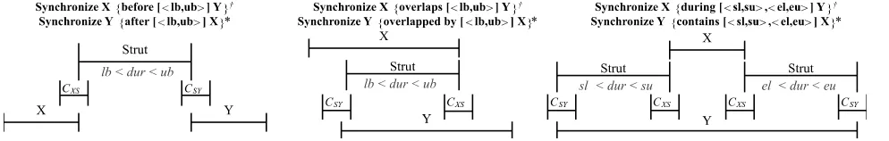
As noted earlier, we can enforce all DDLtemporal relations by constraining the time between the starts and ends of snap-actions. To compile this we can useclips(Fox, Long, and Halsey 2004). With reference to Figure 3 (left), each clip has one or more pair(s) of start and end preconditions that requireone or more snap actions to be applied during the clip (here,x∈eff+_`(X)andeff−_a(X)); and a pair of effects (hereCXY and¬CXY) thatrestrictsome snap action(s) (to

whichCXY is added as a precondition) so that it can only be applied during the clip. When a synchronization places a constraint betweenX andY, but not with itself – or ifX

andY are goals subject to a constraint – then both X and Y must happen at least once, and there must be one pair X,Y that satisfies the constraint. In this case we use a clip that requiresboth X and Y butrestrictsneither, and additionally adds a fact at the end (e.g. metXY) to represent that the

constraint is satisfied: this fact becomes a goal of the PDDL problem, or an end-condition of the action corresponding to the synchronization, as applicable.

Figure 3 (left), demonstrates how we can enforce synchronize X {MET BY Y}(for Y to start, X must end) us-ing a clip that requires X and restricts Y. Soundness fol-lows from the fact that Y cannot be executed outside the clip (due to precondition CXY) and the clip cannot

exe-Figure 3: Compilation Components (note ClipXY,cXY and

Strut are parameterised to make a unique clip/strut for each pair of ground actions, parameters omitted here for clarity).

cute unless X ends within it (due to preconditionsx(start) and¬x(end)). If we want to enforce the inverse relation-ship,synchronize X {MEETS Y}, we instead make the clip restrictXaandrequireY`. This mechanism for synchroniz-ing two snap actions allows us capture to all of the qualita-tive Allen Relations:X MEETS YclipsXatoY`;X STARTS Y clipsX`toY`; andX ENDS YclipsXatoYa. Inverse rela-tions are obtained by swappingXa/`withY`/a.If the condi-tion with respect to Y appears insidesynchronize X{...}, then we use a clip thatrequiresY andrestrictsX.

To model quantitative constraints we use the structure in Figure 3 (right) comprising two clips and astrut. Our strut is inspired by Halseyet al. (2004) but we add a flexible du-ration (lb ≤dur≤ ub), allowing us to enforce both lower and upper bounds on the interval between two snap actions using one action. The start/end of the strut are respectively clipped to snap actionsA1andA2. C1requiresA1and re-strictsstrut`;C2requiresstrutaandrestrictsA2. Hence,A2

can only occur[lb, ub]afterA1: A2can only be applied if clipped to struta; and strut`had to be clipped toA1.

Figure 2 shows the compilation of quantitative con-straints. The constraint enforced is determined by the clips as for qualitative constraints. Clips that requireXandY but restrict neither are used if a synchronization places a con-straint between X andY, but not with itself; or ifX and

Y are goals. If a constraint appears in a synchronize block for X or Y itself (e.g. sync X {BEFORE [lb,ub] Y}) the clips require/restrictX andY as described in the caption. The compilation can streamlined whenlb=0or ub=∞, e.g. sync X {BEFORE [0,INF] Y}, it suffices to add a dummy goal that is true initially, deleted byXaand added byY`.

5 Evaluation

(7)

Table 3: Time (in seconds) taken to solve problems in Domains with Interval constraints, with native handling (nat) versus the compilation (comp). ‘-’ indicates that the problem was unsolved, ’x’ that the problem does not exist.

written in DDLfor an ESA project and translated to PDDL using the methods described in this paper. This allows us to show not only that we now have an efficient native mech-anism for handling Allen Constraints in PDDL, but also to make the case that PDDLplanners can be competitive when it comes to solving space related problems, traditionally handled using timeline based approaches.

We compared the performance of our native approach, the compilation andMTPon the following PDDLdomains. For MTP, these were translated to MPDDL. Concrete (new): Trucks transport concrete, maintaining the liquid state by mixing. The mixing action must occur [2,10] minutes after initially combining the ingredients, and must meet the action to offload concrete. All instances have 2 trucks and scale from delivering concrete to 2–6 sites. Crewplanning (IPC 2008): A domain involving planning the daily routine of as-tronauts. We added constraints that astronauts must have a meal 15–300 minutes after waking up, and exercise at least 30 minutes before going to bed. Zeno Travel (IPC 2000): Passengers must be transported via plane to specific goal air-ports. We added interval constraints to require that aircraft must leave an airport 20–30 minutes after arriving. Cafe (Halsey 2004): Orders placed in a cafe must be prepared and delivered. We added a constraint that food is delivered 1–3 minutes after cooking.

The challenges posed by interval constrainst vary in our domains: in Concrete, solution plans can be padded to satisfy interval constraints; whereas in other domains straints change the structure of solution plans, e.g. the con-straint that crew must eat within an interval after waking: searching without considering interval constraints would yield plans that could not be scheduled to satisfy them.

Our results in Table 3, show that while the compilation has the expressivity to model temporal relations, it is not feasible for solving larger problems as it introduces a large number of additional actions. These increase the branching factor, and lengthen the solution plans the planner must find. Further, they make it much more likely there is a currently executing action in a state, hence memoisation pruning has to be much more conservative (Coles and Coles 2016). This

overhead is incurred by the compilation even in the Concrete domain, where the interval constraints should not, in theory, pose a significant challenge to solving the problem

The native approach significantly outperforms the com-pilation by an order of magnitude (sometimes several). In-deed, any problem solvedat allby the compilation is solved by the native approach in under 2 seconds; and the na-tive approach scales significantly beyond the compilation’s limits. Whilst MIP in general is NP-Hard, the MIPs gen-erated during planning are relatively small and simple so this is not an issue for the native approach in practice: MIP building/solving remains <15% of planner runtime and is dwarfed by heuristic computation time as in prior work (Coles et al. 2012). We note that, while the na-tive approach cannot handle the largest Crewplanning and Zeno problems, this is not because interval constraints hin-der search; but rather that these competition problems are challenging for OPTICeven without additional constraints.

Although MTP can reason with interval constraints en-coded inMPDDL, it was initially unable to solve any of the benchmark problems. This is because it relies on a prede-fined discretization of time that is not fine enough to ad-mit solutions to the problems; i.e. it cannot satisfy tightly bounded interval constraints (e.g. the [1,3] interval in Cafe). We cannot change the discretization as the source code is un-available. To giveMTPa chance to solve these problems we divided all durations and temporal constraints by 10. This does not affect the performance of the native approach, or compilation but allowedMTPto solve some problems; these are the results shown forMTPin Table 3. Even with this scal-ing to suit its discretization, our native approach solves many more problems and solves mutually solved problems at least an order of magnitude faster thanMTP. In fact,MTPis gen-erally outperformed even by the compilation. The makespan of plans produced by MTP were often much longer, and never better, than our approach.

(8)

domain as there are no available standard benchmarks for timeline based planning. The rover must take pictures at certain waypoints, and periodically transmit them. The con-straints on taking a picture are as Figure 1. Data transmis-sion involves three interval relations. The rover must stay at a designated positionduring(and some time before and after) transmission by the antenna; the image must be taken a specified intervalbeforeit is transmitted; and the antenna can only be turned on to transmitduringa communication window, and the rover’s position must be syncronized dur-ingthe antenna being switched on. We defined three groups of problems: the first problems (1-6) involve totally ordered goals limited to taking pictures at waypoints. The second (7-12) additionally require a communication activity for each picture; the third (13-18) are equivalent to 7-12, but with no temporal ordering between the goals. We created 6 problems in each group by increasing the number of images taken and the number of locations (both ranging from 2 to 7).

APSIis faster than OPTIConly on the simplest problems (1-6), where no communication is required, scaling better as problem size increases. In more complex problems (7-12), OPTICclearly outperforms APSI, solving within min-utes problems unsolved by APSI after 30 minutes. Inter-estingly, OPTIC performs better in problems 13-18 where goals are not ordered because when the total ordering is contrary to the search guidance provided by the heuristic, this leads to more of the state space being explored. Con-versely, APSIperforms much worse here: if a goal ordering is given, it is used to guide search. While the compilation did not solve any Rover evaluation problems, in smaller tests it could achieve a single goal of taking a picture at the initial location, or to be at another location, but not to both travel and take a picture. Again, neither planner is attempting to optimise a specific metric, but for interest, we note that both planners produce identical plans for all solved problems.

Acknowledgments

This work has received funding from the European Union’s Horizon 2020 Research and Innovation programme (Grant Agreement 730086, ERGO); EPSRC grant EP/P008410/1 (AI Planning with Continuous Non-Linear Change); the European Space Agency (ESA/ESTEC) GOTCHA project, Contract No. 4000117648/16/NL/GLC/fk; and Ministerio de Econom´ıa, Industria y Competitividad TIN2017-88476-C2-2-R and TIN2015-65686-C5.

References

Allen, J. F. 1983. Maintaining knowledge about temporal intervals. Communications of the ACM26:11.

Baier, J.; Bachus; and McIlraith, S. 2007. A heuristic search ap-proach to planning with temporally extended preferences. InIJCAI. Bedrax-Weiss, T.; McGann, C.; Bachmann, A.; Edgington, W.; and Iatauro, M. 2005. Europa2: User and contributor guide.Technical report, NASA Ames Research Center.

Benton, J.; Coles, A. J.; and Coles, A. I. 2012. Temporal planning with preferences and time-dependent continuous costs. InICAPS. Cesta, A., and Oddi, A. 1996. DDL.1: A formal description of a constraint representation language for physical domains. New Directions in AI Planning.

Cesta, A., and Oddi, A. 2004. Planning with concurrency, time and resources: A CSP-based approach.Intel. Techniques for Planning. Cesta, A., and Oddi, A. 2008. Unifying planning and scheduling as timelines in a component-based perspective.Arc. Control Sciences. Cesta, A.; Fratini, S.; Orlandini, A.; and Rasconi, R. 2012. Con-tinuous planning and execution with timelines. InInternational Symposium on Artificial Intelligence.

Chien, S.; Rabideau, G. R.; Knight, R. L.; Sherwood, R.; Engel-hardt, B.; Mutz, D.; Estlin, T. A.; Smith, B.; Fisher, F. W.; Barrett, A. C.; Stebbins, G.; and Tran, D. 2000. Aspen - automated plan-ning and scheduling for space mission operations. InSpace Ops. Coles, A. J., and Coles, A. I. 2016. Have I Been Here Before? State Memoisation in Temporal Planning. InProc. ICAPS. Coles, A. J.; Coles, A. I.; Fox, M.; and Long, D. 2012. COLIN: Planning with Continuous Linear Numeric Change.JAIR44. Cushing, W.; Kambhampati, S.; Mausam; and Weld, D. 2007. When is temporal planning really temporal planning? InIJCAI. Dechter, R.; Meiri, I.; and Pearl, J. 1991. Temporal constraint networks.Artificial Intelligence49:61–95.

Dvorak, F.; Bart´ak, R.; Bit-Monnot, A.; Ingrand, F.; and Ghallab, M. 2014. Planning and Acting with Temporal and Hierarchical Decomposition Models. InICTAI, 115–121.

Edelkamp, S.; Jabbar, S.; and Nazih, M. 2006. Large-Scale Opti-mal PDDL3 Planning with MIPS-XXL. InIPC5 booklet, ICAPS. Fox, M., and Long, D. 2003. PDDL2.1: An extension ofPDDLfor expressing temporal planning domains.JAIR20.

Fox, M.; Long, D.; and Halsey, K. 2004. An investigation into the expressive power ofPDDL2.1. InProceedings ECAI.

Frank, J. D., and Jonsson, A. K. 2003. Constraint-based attribute and interval planning.Journal of Constraints8:4.

Gerevini, A. E.; Long, D.; Haslum, P.; Saetti, A.; and Dimopoulos, Y. 2009. Deterministic Planning in the Fifth IPC: PDDL3 and Experimental Evaluation of the Planners.AIJ.

Gigante, N.; Montanari, A.; Mayer, M. C.; and Orlandini, A. 2016. Timelines are expressive enough to capture action-based temporal planning. InProc. TIME 2016.

Ocon, J.; Delfa, J. M.; de la Rosa, T.; Garc´ıa, A.; and Escudero, Y. 2017. Gotcha: An autonomous controller for the space domain. In Proc. ASTRA.

Sherwood, R.and Engelhardt, B.; Rabideau, G.; Chien, S.; and Knight, R. 2005. Aspen user’s guide.Tech. Report D15482, JPL. Smith, D. E.; Frank, J.; and Cushing, W. 2008. The ANML lan-guage. InKEPS Workshop, ICAPS.

Smith, D. E. 2003. The Case for Durative Actions: A Commentary on PDDL2.1.JAIR.

Tierney, K.; Coles, A. J.; Coles, A. I.; Kroer, C.; Britt, A.; and Jensen., R. M. 2012. Automated planning for liner shipping fleet repositioning. InProc. ICAPS.

To, S.; Roberts, M.; Apker, T.; Johnson, B.; and Aha, D. 2016. Mixed propositional metric temporal logic: A new formalism for temporal planning. InAAAI Hybrid Systems Workshop.

To, S.; Johnson, B.; Roberts, M.; and Aha., D. 2017. A new ap-proach to temporal planning with rich metric temporal properties. InProc. ICAPS.