SVM-Based Deep Stacking Networks

(1)

The Thirty-Third AAAI Conference on Artificial Intelligence (AAAI-19)

SVM-Based Deep Stacking Networks

Jingyuan Wang,

†,§

_{Kai Feng,}

†

_{Junjie Wu}

‡,§∗

†MOE Engineering Research Center of Advanced Computer Application Technology, School of Computer Science Engineering, Beihang University, Beijing 100191, China

‡Beijing Key Laboratory of Emergency Support Simulation Technologies for City Operations, School of Economics and Management, Beihang University, Beijing 100191, China

§Beijing Advanced Innovation Center for Big Data and Brain Computing, Beihang University, Beijing 100191, China

Email:{jywang, fengkai, wujj}@buaa.edu.cn

Abstract

The deep network model, with the majority built on neural networks, has been proved to be a powerful framework to represent complex data for high performance machine learn-ing. In recent years, more and more studies turn to non-neural network approaches to build diverse deep structures, and the Deep Stacking Network (DSN) model is one of such approaches that uses stacked easy-to-learn blocks to build a parameter-training-parallelizable deep network. In this pa-per, we propose a novel SVM-based Deep Stacking Network (SVM-DSN), which uses the DSN architecture to organize linear SVM classifiers for deep learning. A BP-like layer tun-ing scheme is also proposed to ensure holistic and local opti-mizations of stacked SVMs simultaneously. Some good math properties of SVM, such as the convex optimization, is intro-duced into the DSN framework by our model. From a global view, SVM-DSN can iteratively extract data representations layer by layer as a deep neural network but with paralleliz-ability, and from a local view, each stacked SVM can con-verge to its optimal solution and obtain the support vectors, which compared with neural networks could lead to interest-ing improvements in anti-saturation and interpretability. Ex-perimental results on both image and text data sets demon-strate the excellent performances of SVM-DSN compared with some competitive benchmark models.

Introduction

Recent years have witnessed the tremendous interests from both the academy and industries in building deep neu-ral networks (Hinton and Salakhutdinov 2006; Bengio, Courville, and Vincent 2013). Many types of deep neu-ral networks have been proposed for classification, regres-sion and feature extracting tasks, such as Stacked Denois-ing Autoencoders (SAE) (Vincent et al. 2010), Deep Be-lief Networks (DBN) (Hinton 2011), deep Convolutional Neural Networks (CNN) (Krizhevsky, Sutskever, and Hin-ton 2012), Recurrent Neural Networks (RNN) (Medsker and Jain 2001), and so on.

Meanwhile, the shortcomings of neural network based deep models, such as the non-convex optimization, hard-to-parallelizing, and lacking model interpretation, are get-ting more and more attentions from the pertinent research

∗

Corresponding author

societies. Some potential solutions have been proposed to build deep structure models using non neural network ap-proaches. For instance, in the literature, the PCANet build a deep model using an unsupervised convolutional prin-cipal component analysis (Chan et al. 2015). The gcFor-est builds a tree based deep model using stacked random forests, which is regarded as a good alternative to deep neu-ral networks (Zhi-Hua Zhou 2017). Deep Fisher Networks build deep networks by stacking Fisher vector encoding into multiple layers (Simonyan, Vedaldi, and Zisserman 2013).

Along this line, in this paper, we propose a novel SVM-based Deep Stacking Network (SVM-DSN) for deep ma-chine learning. On one hand, SVM-DSN belongs to the com-munity of Deep Stacking Networks (DSN), which consist of many stacked multilayer base blocks that could be trained in a parallel way and have comparable performance with deep neural networks (Deng and Yu 2011; Deng, He, and Gao 2013). In this way, SVM-DSN can gain the deep learning ability with extra scalability. On the other hand, we replace the traditional base blocks in a DSN,i.e., the perceptrons, by the well known Support Vector Machine (SVM), which has long been regarded as a succinct model with appealing math properties such as the convexity in optimization, and was considered as a different method to model complicated data distributions compared with deep neural networks (Bengio and others 2009). In this way, SVM-DSN can gain the abil-ity in anti-saturation and enjoys improved interpretabilabil-ity, which are deemed to be the tough challenges to deep neu-ral networks. A BP-like Layered Tuning (BLT) algorithm is then proposed for SVM-DSN to conduct holistic and local optimizations for all base SVMs simultaneously.

Compared with the traditional deep stacking networks and deep neural networks, the SVM-DSN model has the follow-ing advantages:

• The optimization of each base-SVM is convex. Using the proposed BLT algorithm, all base-SVMs are optimized as a whole, and meanwhile each base-SVM can also con-verge to its own optimum. The final solution of SVM-DSN is a group of optimized linear SVMs that are in-tegrated as a deep model. This advantage allows SVM-DSN to avoid the neuron saturation problem in deep neu-ral networks, and thus could improve the performance.

(2)

…

… … … …

… … …

… …

… … …

… …

…

… …

…

… … … …

𝑊𝑊1

𝑈𝑈1

𝑊𝑊2

𝑈𝑈2

𝑈𝑈3

𝑈𝑈4

𝑊𝑊3

𝑊𝑊4

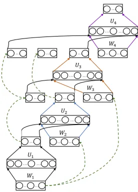
Figure 1: An illustration of the DSN architecture (Deng, He, and Gao 2013). The color is used to distinguish different blocks in a DSN. The components in the same color belong to the same block.

training parallelization in SVM-DSN can reach the base-SVM level due to the support vectors oriented property of SVM, but the traditional DSN can only reach the block level.

• The SVM-DSN model has improved interpretability. The support vectors in base-SVMs can provide some insight-ful information about what a block learned from train-ing data. This property empowers users to partially un-derstand the feature extracting process of the SVM-DSN model.

Experimental results on image and sentiment classifica-tion tasks show that SVM-DSN model obtains respectable improvements over neural networks. Moreover, compared with the stacking models with strong base-learners, the SVM-DSN model also demonstrates significant advantages in performance.

The SVM-DSN Model

Framework of Deep Stacking Network

The Deep Stacking Network is a scalable deep machine learning architecture (Deng, He, and Gao 2013; Deng and Yu 2011) that consists of stacked easy-to-learn blocks in a layer by layer manner. In the standard DSN, a block is a simplified multilayer perceptron with a single hidden layer. Let the inputs of a block be a vector x, the block uses a connection weight matrixW to calculate the hidden layer vectorhas

h=ϕ W>x

, (1)

whereϕ(x) = 1/(1 + exp(−x))is a sigmoid nonlinear ac-tivation function. Using a weight matrix U, the objective function of the DSN block optimization is defined as

miny−U>h

2

F. (2)

As shown in Fig. 1, the blocks of a DSN are stacked layer by layer. For the block in the input layer, the input vectorx contains only the raw input features. For blocks in the mid-dle layers,xis a concatenated vector of the raw input fea-tures and output representations of all previous layer blocks. The training of deep stacking networks contains two steps: block training and fine-tuning. In the block training step, the DSN blocks are independently training as super-vised multilayer perceptrons. In the fine-tuning step, all the stacked blocks are considered as a multi-layer deep neural network. The parameters of DSN are end-to-end trained us-ing the error Back Propagation (BP) algorithm.

SVM-based DSN Blocks

In the SVM-DSN model, we adopt support vector machines to implement a DSN block. A SVM classifier is a hyperplane ω>x+b= 0that divides the feature space of a data sample xinto two parts — one for the positive and the other for the negative. The parametersωandbare optimized to maximize the minimum distances from the hyperplane to a set of train-ing samplesT ={(xk, yk)|yk ∈ {−1,1}, k = 1, . . . , K}, i.e.,

max

ω,b

2

kωk

s.t. yk(ω>xk+b)≥1, k= 1,2, . . . , N. (3)

A training sample is called asupport vectorif the constraint in Eq. (3) turns into equality.

For a multi-class problem withN classes, we connect the input vectorxof a DSN block withN binary SVM classi-fiers — each for recognizing whether a sample belongs to a corresponding class — to predict the label of a sample. A binary SVM classifier in a DSN block is called abase-SVM. TheNbinary SVM classifiers for aNclassification problem is called as abase-SVM group. A SVM-DSN block could contains multiple base-SVM groups. In the same block, all base-SVM groups share the same input vectorx.

Stacking Blocks

Given a classification hyperplane of a SVM, the decision function for the samplexkis expressed as

f(xk) = sign ω>xk+b

, (4)

wheref(xk) = 1for the positive class andf(xk) = −1 for the negative. The distance from a sample to the hyper-plane could be considered as the confidence of a classifi-cation decision. For the samples behind the support vec-tors, i.e.,ω>xk+b

> 1, the confidence is 1, otherwise

isω>xk+b

. We therefore can express the classification

confidence of a SVM classifier for the samplexkas

g(xk) = min 1,|ω>xk+b|

. (5)

We denote thei-th base-SVM in the layerl assvm(l, i) and its decision function and confidence as f(l,i)₍_·₎ _and

g(l,i)₍_·₎_{, respectively. For the base-SVM} _svm₍_{l, i}₎_{, we}

de-fine aconfidence weighted outputy(l,i)_as

(3)

In the layer l+1, SVM-DSN concatenates the confidence weighted outputs of all base-SVMs in the previous layers and raw inputs as

x(l+1)=y(l,1), . . . , y(l,i), . . . , y(l−1,1), . . . , y(l−1,i),

. . . , y(1,1), . . . , y(1,i), . . . , x(1,1), . . . , x(1,i)

>

.

(7) The base-SVMs in the layerl+1 usex(l+1)as the input to generate their confidence weighted outputsy(l+1,i). In this way, base-SVMs are stacked and connected layer by layer.

Model Training

Block Training

Similar to the standard deep stacking network, the training of the SVM-DSN model also contains a block training step and a fine-tuning step.

In the block training step, the base-SVMs in a DSN block are trained as regular SVM classifiers. Given a set of training samples T = {(xk, yk)|k = 1, . . . , K}, whereyk is the ground-truth label of xk, the objective function of a base-SVM group withNclassification is defined as

J =1 2kΩk

2

F

+C

K

X

k=1

N

X

i=1

`hinge

y_k(i)(ω(i)>xk+b(i))

,

(8)

whereΩ= ω(1)>_{, . . . ,}_ω(N)>

, andy(_ki)= 1ifyk=iand -1 otherwise. The function`hinge(·)is a hinge loss function defined as`hinge(z) = max (0,1−z). The parameterθ =

(ω(i)_{, b}(i)₎_|∀_i _{is inferred as}_θ_{= arg min}

θ J(θ).

In order to increase the diversity of base-SVM groups in a block, we adopt a bootstrap aggregating method in the block training. For a block withM base-SVM groups, we re-sample the training data as M sets using the bootstrap method (Efron and Tibshirani 1994). Each base-SVM group is trained using one re-sampled data set.

Fine Tuning

The traditional DSN model is based on neural networks and uses the BP algorithm in the fine-tuning step. For the SVM-DSN model, we introduce SVM training into the BP algo-rithm framework, and propose a BP-like Layered Tuning (BLT) algorithm to fine-tune the model parameters.

Algorithm 1 gives the pseudocodes of BLT. In general, BLT iteratively optimizes the base-SVMs from the output layer to the input layer. In each iteration, BLT optimizes

svm(l, i)by firstly generating a set ofvirtualtraining sam-plesT(l,i) ={(x(_kl),y˜(_kl,i))|k = 1, . . . , K}, and then trains a newsvm(l, i)onT(l,i)_.

According to Eq. (6) and Eq. (7), it is easy to havex(_kl)= (y_k(l−1,1), y_k(l−1,2),· · · , y_k(l−1,i),· · ·)>. However, the calcu-lation of thevirtual labely˜(_kl,i) is not that straightforward.

Algorithm 1BP-like Layered Tuning Algorithm

1: Initialization: Initializingω(l,i)_{, b}(l,i) _{for all} _svm₍_{l, i}₎

as random values. 2: repeat

3: Select a batch of training samplesT ={(xk, yk)|k=

1, . . . , K}.

4: forl=L, L−1, . . . ,2,1do

5: fori= 1,2, . . .do

6: Use Eq. (6), Eq. (7), and Eq. (9) to calculate

T(l,i)={(x(_kl),y˜(_kl,i))|k= 1, . . . , K}. 7: UseT(l,i)_{to train}_svm₍_{l, i}₎_{as Eq. (11).}

8: end for

9: end for

10: untilThe algorithm converges.

Specifically, BLT adopts a gradient descent method to cal-culatey˜_k(l,i)as

˜

y_k(l,i)=σ y(_kl,i)−η ∂J

(o)

∂y(l,i)

_y(l,i)₌_y(l,i)

k

!

, (9)

whereJ(o)_{is the objective function of the output layer,}_y(l,i)

k is the output ofx(_kl)in the previous iteration,ηis the learning rate, andσ(·)is a shaping function defined as

σ(z) = 





1, z >1

z, |z| ≤1

−1, <−1

. (10)

Note that since the term−η∂J(o)_/∂y(l,i)_{in Eq. (9) is a}

neg-ative gradient direction of J(o)_{, tuning the output}_y(l,i)_to

the virtual labely˜(l,i)_{can reduce the value of the objective}

functionJ(o)_{in the output layer. Therefore, it could be}

ex-pected that BLT can lower the overall model prediction error iteratively by training base-SVMs on virtual training sets in each iteration.

Given the training set T(l,i) ₌ _{₍_x(l)

k ,y˜

(l,i)

k )|k =

1, . . . K}, the objective function of trainingsvm(l, i)is de-fined as

minJ(l,i)₌1

2

ω

(l,i) 2

+C1 X

k∈Θ

`hinge

˜

y(_kl,i)(ω(l,i)>x(_kl)+b(l,i))

| {z }

The SVM Loss

+C2 X

k /∈Θ

`

ω(l,i)>x(_kl)+b(l,i)−y˜(_kl,i)

| {z }

The SVR Loss

,

(11)

whereΘis the index set of the virtual labels

y˜

(l,i)

k

= 1,

and the function`(·)is an-insensitive loss function in the form of`(z) = max(|z| −,0).

(4)

are binary, BLT trainssvm(l, i)as the standard SVM classi-fier and thus uses the hinge loss function to measure errors. Wheny˜_k(l,i)∈(−1,1), the objective function adopts a Sup-port Vector Regression loss term`for this condition. In the Appendix, we prove that the problem defined in Eq. (11) is a quadratic convex optimization problem. The training of

svm(l, i)can thus reach an optimal solution by using vari-ous quadratic programming methods such as sequential min-imal optimization and gradient descents.

We finally turn to the small problem unsolved — how to calculate the partial derivative ∂J(o)/∂y(l,i)in Eq. (9). Based on the chain rule, the partial derivative can be recur-sively calculated as

∂J

∂y(l,i) =

L

X

m=l+1

X

j

∂J

∂y(m,j)

dy(m,j)

dz(m,j)

∂z(m,j) ∂y(l,i)

=

L

X

m=l+1

X

j

∂J

∂y(m,j)y

0_z(m,j)_ω(m,j)

i , (12)

where ω_i(m,j) is the connection weight of y(m,j) in

svm(m, j), and z(m,j) = ω(m,j)>x(m−1) +b(m,j). The termy0(z)is the derivative of the function in Eq. (6), which is in the form of

y0(z) =

₀_, _|_z_|_>₁

1, |z| ≤1. (13)

The principle of this chain derivation is similar to the error back-propagation of the neural network training. The differ-ence lies in that the BP algorithm calculates the derivative for each neuron connecting weight but BLT for each base-SVM output. That is why we name our algorithm asBP-like Layered Tuning.

Model Properties

Connection to Neural Networks

The SVM-DSN model has close relations with neural networks. If we view the base-SVM output function defined in Eq. (6) as a neuron, the SVM-DSN model can be regarded as a type of neural networks. Specifically, we can rewrite the function in Eq. (6) as a neuron form as follows:

y(l,i)=σω(l,i)>x(l)+b(l,i), (14)

where the shaping functionσ(·)works as an activate func-tion, with the output σ(z) ∈ {1,−1} if |z| ≥ 1, and

σ(z) = z if|z| <1. As proved in (Hornik 1991), a multi-layer feedforward neural network with arbitrary bounded and non-constant activation function has an universal ap-proximation capability. As a consequence, we could expect that the proposed SVM-DSN model also has the universal approximation capability in theory.

Nevertheless, the difference between the SVM-DSN model and neural networks is still significant. Indeed, we have proven in the Appendix that the base-SVMs in our SVM-DSN model have the following property: Given a set of virtual training samples{(x(_kl),y˜_k(l,i))|k= 1, . . . , K}for

svm(l, i), to minimize the loss function defined in Eq. (11) is a convex optimization problem. Moreover, because the base-SVMs in the same block are mutually independent, the optimization of the whole block is a convex problem too. This implies that, in each iteration of the BLT algorithm, all blocks can converge to an optimal solution. In other words, SVM-DSN ensures that all blocks and their base-SVMs “do their own best” to minimize their own objective functions in each iteration, which however is not the case for neural networks and MLP based deep stacking networks. It is also worth noting that this “do their own best” property is compatible with the decrease of the overall prediction error measured by the global objective functionJ(o)_.

An important advantage empowered by the “do their own best” property is theanti-saturationfeature of SVM-DSN. In neural network models, the BP algorithm updates the pa-rameterωof a neuron asω ←η∂J/∂ω. Hence, the partial derivative for thei-thωin thej-th neuron at the layerl is calculated as

∂J ∂ω_i(l,j)

= ∂J

∂y(l,j)

dy(l,j)

dz(l,j)

∂z(l,j)

∂ω_i(l,j)

= ∂J

∂y(l,j)·y

0_z(l,j)_·_y(l−1,i)_,

(15)

wherey0 z(l,j) is a derivative of the activation function. For the sigmoid activation function, if|z|is very large then

y0 becomes very small, and∂J /∂ω →0. In this condition, the BP algorithm cannot updateωany more even if there is still much room for the optimization ofω. This phenomenon is called the “neuron saturation” in neural network training. For the ReLU activation function, similar condition appears when z < 0, wherey0 = 0and∂J /∂ω = 0. The neuron will die when a ReLU neuron fall into this condition.

In the BLT algorithm of SVM-DSN model, the update of a base-SVM is guided by∂J/∂y, with the details given in Eq. (12). From Eq. (12), we can see that unless all base-SVMs in an upper layer are saturated,i.e.,y0(z(m,j)_{) = 0}_for

allz(m,j)_{, the base-SVMs in the layer}_l_{would not fall into}

the saturation state. Therefore, we could expect that the sat-uration risk of a base-SVM in SVM-DSN tends to be much lower than a neuron in neural networks.

Interpretation

(5)

(a) Layer-1 (b) Layer-2 (c) Layer-3

Figure 2: The classifying plane maps of each layer in the SVM-DSN.

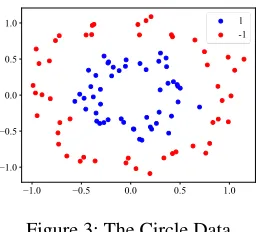
Figure 3: The Circle Data

“classifying plane” maps layer by layer, we could partly un-derstand the feature extracting process of the stacked block in a SVM-DSN model.

We here give a show case to explain the interpretation property of SVM-DSN in a direct way. In this case, we gen-erate a circle data set containing samples of two classes, as shown in Fig. 3. The positive samples are generated from a circle with radius of 0.5 plus a Gaussian noise with vari-ance of 0.1. The negative samples are generated from a circle with radius of 1 plus the same Gaussian noise. We use the circle data set to train a 3-layer SVM-DSN model, where the middle layers contain 40 and 60 base-SVM groups, respec-tively. Because this experiment is a binary classification, a base-SVM group only contains one base-SVM.

In the experiment, we traverse the feature space from the coordinate point (−2,−2) to (2,2). For each coordinate point, we calculate the average confidence of all base-SVMs in each layer. Figs. 2a - 2c plot the confidence distribution maps in different layers. The samples with low confidence are thus near to the SVM classification hyperplane, so the low confidence areas in red form the “classifying plane” of a layer.

It is obvious that there is a clear “classifying plane” gen-eration process from Figs. 2a to 2c. In the layer 1, the low confidence values concentrate in the center of the map. In the layer 2, the low confidence values have a vague shape as a circle. In the layer 3, the low confidence values distribute as a circle shape that clearly divides the feature space into two parts. This process demonstrates how an SVM-DSN model extracts the data representations of the feature space layer by layer.

Parallelization

The deep stacking network is proposed for parallel param-eter learning. For a DSN withL blocks, given a group of

training samples, the DSN can resample the data set as L

batches. A DSN block only uses one batch to update its pa-rameter. In this way, the training of DSN parameters could be deployed overLprocessing units. The parallelization of DSN training is in the block level.

This parallel parameter learning property could be further extended by using Parallel Support Vector Machines (Graf et al. 2005). Because in a SVM classifier, only the support vector samples are crucial, we could divide a training set as severalMsub-sets, and useMvirtual SVM classifiers to se-lect support vector candidates from each sub-set. Finally, we use the support vector candidates of all sub-sets to train the final model. In this way, the training of a SVM-DSN block can be deployed overM processing units, and the all SVM-DSN model can be deployed overL×Mprocessors. That is to say the training of base-SVMs in a block is also paralleliz-able in SVM-DSN. The parallelization of SVM-DSN train-ing is in the base-SVM level. The parallel degree of whole model is greatly improved. As reported in Ref (Graf et al. 2005), the speed-up for a 5-layer Cascade SVM (16 parallel SVMs) to a single SVM is about 10 times for each pass and 5 times for fully converged.

Experiments

Image Classification Performance

(6)

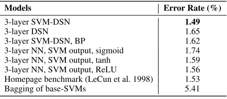
Table 1: MNIST Classification Performance

Models Error Rate (%)

3-layer SVM-DSN 1.49

3-layer DSN 1.65

3-layer SVM-DSN, BP 1.62

3-layer NN, SVM output, sigmoid 1.74 3-layer NN, SVM output, tanh 1.59 3-layer NN, SVM output, ReLU 1.56 Homepage benchmark (LeCun et al. 1998) 1.53

Bagging of base-SVMs 5.41

the different activate functions in neurons;iv) The best layer NN benchmark listed in the homepage of MNIST – 3-layer NN, 500+300 hidden units, cross entropy loss, weight decay (LeCun et al. 1998);v) A bagging of 41 base-SVM groups, each group contains 10 base-SVMs.

In the SVM-DSN model fine-tuning, we have two hyper-parameters to set,i.e.,C1andC2of the base-SVM’s objec-tive function. The two hyper-parameters are used to balance structural risks and empirical risks in a base-SVM. Either too big or too small for the two hyper-parameters may lead model performance degenerate. Therefore, we use the trial and error method to set the hyper-parameters. The learn-ing rateη is the other hyper-parameter, which could be dy-namic setting using elegant algorithms such as Adam. In our experiment, we directly set the learning rate as a fix value

η= 0.0005to ensure the experiment fairness.

Table 1 gives the MNIST image classification results. The SVM-DSN model achieved the best performance com-pared with the other benchmarks, which verified the ef-fectiveness of SVM-DSN. In the benchmarks, the 3-layer SVM-DSN+BP model has the same model structure with SVM-DSN but was trained by the BP algorithm. The results show that SVM-DSN has a better performance than the SVM-DSN+BP benchmark, which indicates that the base-SVMs “do their own best” feature of SVM-DSN is a posi-tive feature for model performance. In fact, the idea of BLT fine-tuning could be extend to optimize the deep stacking networks with any derivable model as blocks, such as soft decision-making tree and linear discriminant analysis.

Feature Extractor Compatibility

Currently, the mainstream image classifiers usually adopt convolutional neural networks (CNN) as feature extractors. Table 2 demonstrates the MNIST classification performance of SVM-DSN with a CNN feature extractor. In the exper-iment, we connect a CNN feature extractor with a 3-layer SVM-DSN model. The structure of SVM-DSN is same as in Table 1. The CNN feature extractor contains 3 convo-lutional layers, and each layer consists of 24 flitters with the 5×5 receptive field. In the CNN and SVM-DSN mix-ture model, we first pre-trained the CNN part using BP, and then uses the feature extracted by CNN as input of the SVM-DSN part to train the blocks. In the fine-tuning step, the CNN part is fine tuned by BP and the SVM-DSN part is tuned by BLT. The benchmark models include:i) The same CNN feature extractor connected with a 3-layer DSN, where

Table 2: MNIST Classification with CNN Feature Extractor

CNN + SVM-DSN 0.51

CNN + DSN 0.60

CNN + SVM-DSN, BP 0.72

CNN + sigmoid activation 0.80

CNN + tanh activation 0.67

CNN + ReLU activation 0.58

Homepage benchmark (LeCun et al. 1998) 0.54 gcForest (Zhi-Hua Zhou 2017) 0.74

Table 3: IMDB Classification Performance

SVM-DSN 10.51

DSN 11.15

SVM-DSN, BP 11.42

Random Forest 14.68

XGBoost 14.77

AdaBoost 16.63

SVM (linear kernel) 12.43

Stacking 11.55

Bagging of base-SVMs 11.66

gcForest (Zhi-Hua Zhou 2017) 10.84

the 3-layer DSN has the same structure with the 3-layer SVM-DSN model;ii) The CNN+SVM-DSN model trained by the BP algorithm;iii) The neural networks consist of 3 CNN layers and 3-layer neural network with different acti-vate functions, where the structures of the CNN and the neu-ral network are same as the CNN + SVM-DSN model;iv) The trainable CNN feature extractor + SVMs with affine dis-tortions, which is the best benchmark with the similar mod-els scale listed in the MNIST homepage; v) The gcForest with convolutional kernels (Zhi-Hua Zhou 2017). As shown in Table 2, the CNN + SVM-DSN model achieved the best performance, which verified the effectiveness of our model again. What’s more, this experiment demonstrates that the SVM-DSN model is completely compatible to the neural network framework. The other types of networks, such as RNN and LSTM, could also be used as feature extractors of SVM-DSN to adapt diversified application scenarios.

Comparison with Ensemble Models

(7)

base-SVMs in the middle layer are 1024-1024-512-256. The benchmark models include Random Forest, XGBoost, Ad-aBoost and SVM (linear kernel). The four benchmarks are also stacked as a stacking benchmark (Perlich and ´Swirszcz 2011). A bagging of base-SVMs and the grForest (Zhi-Hua Zhou 2017) are also included as competitor. A 4-layer DSN is used as a benchmark, where the number of hidden neurons in the middle layer blocks are same as the number of base-SVMs in the SVM-DSN model. The SVM-DSN model trained by the BP algorithm is also used as the benchmark.

As shown in Table 3, the SVM-DSN model achieved the best performance again. Especially, the performance of SVM-DSN is better than the stacking benchmark, which in-dicates that holistic optimized multi-layer stacking of linear base-learners can defeat the traditional two-layer stacking of strong base-learners. In the experiment, the performance of the BLT algorithm is yet better than the BP algorithm. The “do their best” feature of base-SVM in BLT is still effective in text sentiment classification.

Related Works

This work has close relations with SVM, deep learning, and stacking. The support vector machine was first pro-posed by Vapnik in (Vapnik 1998). Multi-layer structures in SVM were usually used as speedup solutions. In cas-cade SVM (Graf et al. 2005), a multi-layer cascas-cade SVM model structure was used to select support vectors in a par-allel way. In the literature (Collobert, Bengio, and Bengio 2002), a parallel mixture stacking structure was proposed to speed up SVM training in the very large scale problems. Be-fore our work, some studies proposed to use SVM to replace the output layer of a neural network (Wiering et al. 2013; Tang 2013).

In recent years, neural network based deep models has achieved great success in various applications (Hinton and Salakhutdinov 2006). The gcFroest model (Zhi-Hua Zhou 2017) was proposed to use the forest based deep model as an alternative to deep neural networks. The PCANet builds a deep model using unsupervised convolutional principal component analysis (Chan et al. 2015). LDANet is a super-vised extension of PCANet, which uses linear discriminant analysis (LDA) to replace the PCA parts of PCANet (Chan et al. 2015). Deep Fisher Networks build deep network through stacking Fisher vector encoding as multi-layers (Si-monyan, Vedaldi, and Zisserman 2013).

The DSN framework adopted in this work is a scal-able deep architecture amenscal-able to parallel parameter train-ing, which has been adopted in various applications, such as information retrieval (Deng, He, and Gao 2013), image classification (Li, Chang, and Yang 2015), and speech pat-tern classification (Deng and Yu 2011). T-DSN uses tensor blocks to incorporate higher order statistics of the hidden bi-nary features (Hutchinson, Deng, and Yu 2013). The CCNN model extends the DSN framework using convolutional neu-ral networks (Zhang, Liang, and Wainwright 2016). To the best of our knowledge, there are very few works introduce the advantages of SVM into the DSN framework.

Stacking was introduced by Wolpert in (Wolpert 1992) as a scheme of combining multiple generalizers. In many

real-world applications, the stacking methods were used to integrate strong base-learners as an ensemble model to improve performance (Jahrer, T¨oscher, and Legenstein 2010). In the literature, most of stacking works focused on designing elegant meta-learners and create better base-learners, such as using class probabilities in stacking (Ting and Witten 1999), using a weighted average to combine stacked regression (Rooney and Patterson 2007), training base-learners using cross-validations (Perlich and ´Swirszcz 2011), and applying ant colony optimization to configure base-learners (Chen, Wong, and Li 2014). To the best of our knowledge, there are very few works to study how to opti-mize multi-layer stacked base-learners as a whole.

Conclusion

In this paper, we proposed an SVM-DSN model where linear base-SVMs are stacked and trained in a deep stacking net-work way. In the SVM-DSN model, the good mathematical property of SVMs and the flexible model structure of deep stacking networks are nicely combined in a same frame-work. The SVM-DSN model has many advantage proper-ties including holistic and local optimization, parallelization and interpretation. The experimental results demonstrated the superiority of the SVM-DSN model to some benchmark methods.

Acknowledgments

Prof. J. Wang’ s work was partially supported by the Na-tional Key Research and Development Program of China (No.2016YFC1000307), the National Natural Science Foun-dation of China (NSFC) (61572059, 61202426), the Science and Technology Project of Beijing (Z181100003518001), and the CETC Union Fund (6141B08080401). Prof. J. Wu was partially supported by the National Natural Sci-ence Foundation of China (NSFC) (71531001, 71725002, U1636210, 71471009, 71490723).

Appendix

Property: Given a set of virtual samples T(l,i) ₌ {(x(_kl),y˜_k(l,i))|k = 1, . . . , K}forsvm(l, i), to minimize the

loss function defined in Eq. (11) is a convex optimization

problem.

Proof.For the sake of simplicity, we omit the superscripts

(l)of x_k(l) andy˜_k(l) in our proof. We define a constrained optimization problem in the form of

min

ω,b,ξk,ξˆk,ζk

1 2kωk

2

+C1

X

k /∈Θ

ζk+C2

X

k∈Θ

ξk+ ˆξk

s.t. 1−y˜k ω>xk+b≤ζk, (1)

ζk ≥0, k∈Θ;

ω>xk+b−y˜k≤+ξk, (2)

˜

yk− ω>xk+b

≤+ ˆξk, (3)

ξk ≥0, ξˆk ≥0, k /∈Θ.

(8)

We can see the constrained optimization problem Eq. (16) is in a quadratic programming form as

min

a

1 2a

>_Ua₊_c>_a

s.t. Qa≤p,

(17)

wherea= (ω, b,ξ,ξˆ,ζ), andUis a positive semi-definite diagonal matrix. Therefore, the constrained optimization problem is a quadratic convex optimization problem (Boyd and Vandenberghe 2004). It is easy to prove that the con-strained optimization problem defined in Eq. (16) is equiva-lent to the unconstrained optimization problem defined in Eq. (11) (Zhang 2003). Therefore, the optimization prob-lem of base-SVM is equivalent to the probprob-lem defined in Eq. (16). The optimization problem of base-SVM is a con-vex optimization problem.

References

Bengio, Y., et al. 2009. Learning deep architectures for AI.

Foundations and trends in Machine Learning2(1):1–127.

Bengio, Y.; Courville, A.; and Vincent, P. 2013. Repre-sentation learning: A review and new perspectives. IEEE Transactions on Pattern Analysis and Machine Intelligence

(TPAMI)35(8):1798–1828.

Boyd, S., and Vandenberghe, L. 2004.Convex optimization. Cambridge University.

Chan, T.-H.; Jia, K.; Gao, S.; Lu, J.; Zeng, Z.; and Ma, Y. 2015. PCANet: A simple deep learning baseline for im-age classification? IEEE Transactions on Image Processing 24(12):5017–5032.

Chen, Y.; Wong, M.-L.; and Li, H. 2014. Applying ant colony optimization to configuring stacking ensembles for data mining.Expert Systems with Applications41(6):2688– 2702.

Collobert, R.; Bengio, S.; and Bengio, Y. 2002. A parallel mixture of SVMs for very large scale problems. InNIPS, 633–640.

Deng, L., and Yu, D. 2011. Deep convex net: A scalable architecture for speech pattern classification. In INTER-SPEECH, 2285–2288.

Deng, L.; He, X.; and Gao, J. 2013. Deep stacking networks for information retrieval. InICASSP, 3153–3157. IEEE. Efron, B., and Tibshirani, R. J. 1994.An introduction to the bootstrap. CRC press.

Graf, H. P.; Cosatto, E.; Bottou, L.; Dourdanovic, I.; and Vapnik, V. 2005. Parallel support vector machines: The cascade SVM. InNIPS, 521–528.

Hinton, G. E., and Salakhutdinov, R. R. 2006. Reducing the dimensionality of data with neural networks. Science 313(5786):504–507.

Hinton, G. 2011. Deep belief nets. In Encyclopedia of Machine Learning. Springer. 267–269.

Hornik, K. 1991. Approximation capabilities of multilayer feedforward networks.Neural networks4(2):251–257.

Hutchinson, B.; Deng, L.; and Yu, D. 2013. Tensor deep stacking networks. IEEE Transactions on Pattern Analysis

and Machine Intelligence (TPAMI)35(8):1944–1957.

Jahrer, M.; T¨oscher, A.; and Legenstein, R. 2010. Com-bining predictions for accurate recommender systems. In SIGKDD, 693–702. ACM.

Krizhevsky, A.; Sutskever, I.; and Hinton, G. E. 2012. Imagenet classification with deep convolutional neural networks. InNIPS, 1097–1105.

LeCun, Y.; Bottou, L.; Bengio, Y.; and Haffner, P. 1998. Gradient-based learning applied to document recognition.

Proceedings of the IEEE86(11):2278–2324.

Li, J.; Chang, H.; and Yang, J. 2015. Sparse deep stacking network for image classification. InAAAI, 3804–3810. Maas, A. L.; Daly, R. E.; Pham, P. T.; Huang, D.; Ng, A. Y.; and Potts, C. 2011. Learning word vectors for sentiment analysis. InACL, 142–150.

Medsker, L., and Jain, L. 2001. Recurrent neural networks. Design and Applications.

Perlich, C., and ´Swirszcz, G. 2011. On cross-validation and stacking: Building seemingly predictive models on random data.ACM SIGKDD Explorations Newsletter12(2):11–15. Rooney, N., and Patterson, D. 2007. A weighted combina-tion of stacking and dynamic integracombina-tion. Pattern Recogni-tion40(4):1385–1388.

Simonyan, K.; Vedaldi, A.; and Zisserman, A. 2013. Deep fisher networks for large-scale image classification. InNIPS, 163–171.

Tang, Y. 2013. Deep learning using linear support vector machines. arXiv preprint arXiv:1306.0239.

Ting, K. M., and Witten, I. H. 1999. Issues in stacked generalization. Journal of Artificial Intelligence Research 10:271–289.

Vapnik, V. 1998. Statistical learning theory. 1998. Wiley, New York.

Vincent, P.; Larochelle, H.; Lajoie, I.; Bengio, Y.; and Man-zagol, P.-A. 2010. Stacked denoising autoencoders: Learn-ing useful representations in a deep network with a local de-noising criterion. Journal of Machine Learning Research 11:3371–3408.

Wiering, M.; Van der Ree, M.; Embrechts, M.; Stollenga, M.; Meijster, A.; Nolte, A.; and Schomaker, L. 2013. The neural support vector machine. InBNAIC.

Wolpert, D. H. 1992. Stacked generalization. Neural

networks5(2):241–259.

Zhang, Y.; Liang, P.; and Wainwright, M. J. 2016. Con-vexified convolutional neural networks. arXiv preprint arXiv:1609.01000.

Zhang, T. 2003. Statistical behavior and consistency of clas-sification methods based on convex risk minimization.

An-nals of Statistics32(1):56–134.