The Reduced PC-Algorithm: Improved Causal Structure
Learning in Large Random Networks
Arjun Sondhi∗ [email protected]
Ali Shojaie [email protected]
Department of Biostatistics University of Washington Seattle, WA 98195-4322, USA
Editor:Edo Airoldi
Abstract
We consider the task of estimating a high-dimensional directed acyclic graph, given ob-servations from a linear structural equation model with arbitrary noise distribution. By exploiting properties of common random graphs, we develop a new algorithm that requires conditioning only on small sets of variables. The proposed algorithm, which is essentially a modified version of the PC-Algorithm, offers significant gains in both computational complexity and estimation accuracy. In particular, it results in more efficient and accu-rate estimation in large networks containing hub nodes, which are common in biological systems. We prove the consistency of the proposed algorithm, and show that it also re-quires a less stringent faithfulness assumption than the PC-Algorithm. Simulations in low and high-dimensional settings are used to illustrate these findings. An application to gene expression data suggests that the proposed algorithm can identify a greater number of clinically relevant genes than current methods.
Keywords: causal discovery, directed acyclic graphs, faithfulness, high dimensions, ran-dom graphs
1. Introduction
Directed acyclic graphs, or DAGs, are commonly used to represent causal relationships in complex biological systems. For example, in gene regulatory networks, directed edges represent regulatory interactions among genes, which are represented as nodes of the graph. While causal effects in biological networks can be accurately inferred from perturbation experiments (Shojaie et al., 2014)—including single or double gene knockouts (Schadt et al., 2005; Yoo et al., 2002)—these are costly to run. Estimating DAGs from observational data is thus an important exploratory task for generating causal hypotheses (Friedman et al., 2000; Jansen et al., 2003), and designing more efficient experiments.
Since the number of possible directed graphs grows super-exponentially in the number of nodes, estimation of DAGs is an NP-hard problem (Chickering, 1996). Methods of estimating DAGs from observational data can be broadly categorized into three classes. The first class, score-based methods, search over the space of all possible graphs, and
∗. Arjun Sondhi is currently a Quantitative Scientist at Flatiron Health.
c
attempt to maximize a goodness-of-fit score, generally using a greedy algorithm. Examples include the hill climbing and tabu search algorithms (Scutari, 2010), as well as Bayesian approaches (Eaton and Murphy, 2012). The second class, constraint-based methods, first estimate the graph skeleton by performing conditional independence tests; the skeleton of a directed acyclic graph is the undirected graph obtained by removing the direction of edges. Information from conditional independence relations is then used to partially orient the edges of the graph. The resulting completed partially directed acyclic graph (CPDAG) represents the class of all directed acyclic graphs that are Markov equivalent, and therefore not distinguishable from observational data. The most well-known constraint-based method is the PC-Algorithm (Spirtes et al., 2000), which was popularized by Kalisch and B¨uhlmann (2007) for high-dimensional estimation. Finally, hybrid methods combine score and constraint-based approaches. For example, the Max-Min Hill Climbing algorithm (Tsamardinos et al., 2006) estimates the skeleton using a constraint-based method, and then orients the edges by using a greedy search algorithm. Sparsity-inducing regularization approaches have also been used to develop efficient hybrid methods (Schmidt et al., 2007). Estimating DAGs in high dimensions introduces new computational and statistical chal-lenges. Until recently, graph recovery in high dimensions was only established for the PC-Algorithm (Kalisch and B¨uhlmann, 2007) and hybrid constraint-based methods (Ha et al., 2016). While the recent work of Nandy et al. (2015) extends these results to score-based algorithms and their hybrid extensions, the PC-Algorithm is still considered a gold stan-dard in high-dimensional sparse settings, due to its polynomial time complexity (Kalisch and B¨uhlmann, 2007). Moreover, constraint-based methods are indeed the building blocks of various hybrid approaches. Therefore, we primarily focus on constraint-based methods in this paper.
law graphs are of particular interest in many biological applications, as they allow for the presence of hub nodes.
In this paper, we propose a low-complexity constraint-based method for estimating high-dimensional sparse DAGs. The new method, termed reduced PC (rPC), exploits the local separation property of large random networks, which was used by Anandkumar et al. (2012) in estimation of undirected graphical models. We show that rPC can consistently estimate the skeleton of high-dimensional DAGs by conditioning only on sets of small cardinality. This is in contrast to previous heuristic DAG learning approaches that set an upper bound on the number of parents for each node (Acid and de Campos, 1994; Huete and Campos, 1993), which is an assumption that cannot be justified in many real-world networks. We also show that computational and sample complexities of rPC only depend on average sparsity of the graph—a notion that is made more precise in Sections 3 and 4. This leads to consid-erable advantages over the PC-Algorithm, whose computational and sample complexities scale with the maximal node degree. Moreover, these properties hold for linear structural equation models (Shojaie and Michailidis, 2010) with arbitrary noise distributions, and re-quire a weaker faithfulness conditions on the underlying probability distributions than the PC-Algorithm. We present two version of the rPC algorithm: a “full” version for which we provide theoretical guarantees, and an approximate version which is much faster and performs almost identically in practice.
The rest of the paper is organized as follows. In Section 2 we review basic properties of graphical models over DAGs, and give a short overview of the PC-Algorithm. Our new algorithm is presented in Section 3 and its properties, including consistency in high dimensions are discussed in Section 4. Results of simulation studies and a real data example concerning the estimation of gene regulatory networks are presented in Sections 5 and 6, respectively. We end with a brief discussion in Section 7. Technical proofs and additional simulations are presented in the appendices.
2. Preliminaries
In this section, we review relevant properties of graphical models defined over DAGs, and briefly describe the theory and implementation of the PC-Algorithm.
2.1. Background
For p random variables X1, . . . , Xp, we define a graph G= (V, E) with vertices, or nodes,
V = {1, . . . , p} such that variable Xj corresponds to node j. The edge set E ⊂ V ×V
contains directed edges; that is, (j, k) ∈ E implies (k, j) 6∈E. Furthermore, there are no directed cycles in G. We denote an edge from j to k as j → k and call j a parent of k, and k a child of j. The set of parents of node k is denoted pa(k), while the set of nodes adjacent to it, or all ofk’s parents and children, is denotedadj(k). These notations are also used for the corresponding random variable Xk. We assume there are no hidden common
parents of node pairs (that is, no unmeasured confounders). The degree of nodekis defined as the number of nodes which are adjacent to it, |adj(k)|; we denote the maximal degree in the graph as dmax. A triplet of nodes (i, j, k) is called anunshielded triple ifiand j are
adjacent to k but iand j are not adjacent. An unshielded triple is called a v-structure if
We assume random variables follow a linear structural equation model (SEM),
Xk=
X
j∈pa(k)
ρjkXj+k, (1)
where fork= 1, . . . , p,kare independent random variables with finite variance, andρjk are
fixed unknown constants. The directed Markov property, stated below, is usually assumed in order to connect the joint probability distribution of X1, . . . , Xp to the structure of the
graphG.
Definition 1 A probability distribution is Markov on a DAG G = (V, E) if, conditional
on its parents, every random variable Xk is independent of its non-descendants; that is,
Xk⊥⊥Xj |pa(Xk) for all j∈V which are non-descendants ofk.
Although this assumption allows us to connect conditional independence relationships to the DAG structure, there are generally multiple graphs that generate the same distribution under the Markov property. More concretely, DAGs are Markov equivalent if they have the same skeleton and the same set of v-structures. Therefore, constraint-based methods focus primarily on estimating the skeleton of the DAGs from observational data. Conditional independence relations identified when learning the skeleton are then used to orient some of the edges to obtain the CPDAG, which represents the Markov equivalence class of directed graphs (Kalisch and B¨uhlmann, 2007).
We next define d-separation, a graphical property which is used to read conditional independence relationships from the DAG structure.
Definition 2 In a DAG G, two nodes k1 and k2 are d-separated by a set S if and only if,
for all paths π betweenk1 and k2:
(i) π contains a chain i→m→j or a fork i←m→j such that the middle node m is in
S, or
(ii) π contains an inverted fork (or collider)i→m←j such that the middle nodem is not
in S and no descendant of m is inS.
A pathπwhich does not satisfy the requirements of this definition is known as ad-connecting path. Using observed data, d-separations in a graphGcan be identified based on conditional independence relationships. To this end, we require the following assumption, known as
faithfulness, on the probability distribution of random variable on G.
Definition 3 A probability distribution is faithful to a DAG G if Xi ⊥⊥Xj |XS whenever
iand j are d-separated by S.
2.2. The PC-Algorithm
Together, d-separation and faithfulness suggest a simple algorithm for recovering the DAG skeleton. If we discover that Xi ⊥⊥ Xj | S for some set S, then there cannot be an edge
(i, j) ∈ E. Conversely, if we discover Xi 6⊥⊥ Xj | S for all possible sets S, then there
computationally infeasible for large p, and statistically problematic when p > n, it forms the basis of the PC-Algorithm. The PC-Algorithm starts with a complete undirected graph and deletes edges (i, j) if a setS can be found such that Xi ⊥⊥Xj |S. The algorithm also
uses the fact that if such an S exists, then there exists a set S0 such that all nodes in S0
are adjacent to i or j and Xi ⊥⊥ Xj | S0. Thus, at each step of the algorithm, only local
neighbourhoods need to be examined in order to find the separating sets.
Although consistent for sufficiently sparse high-dimensional DAGs, the PC-Algorithm’s computational and sample complexity scale with the maximal degree of the graph, dmax.
Specifically, the algorithm’s computational complexity isO pdmaxand its sample complex-ity is Ω
max(logp, d1max/b ) for some b∈(0,1]. This is problematic for graphs with highly
connected hub nodes, which are common in real-world networks (Chen and Sharp, 2004; Jeong et al., 2000). In such graphs, dmax typically grows with the number of nodes p,
leading to poor accuracy and runtime for the PC-Algorithm.
Another limitation of the PC-Algorithm is that it requires partial correlations between adjacent nodes to be bounded away from 0; this requirement, which needs to hold for all conditioning setsS such that |S| ≤dmax, is known asrestricted strong faithfulness (Uhler
et al., 2013), and is defined next.
Definition 4 Given λ∈(0,1), a distribution P is said to be restricted λ-strong-faithful to
a DAGG= (V, E) if the following conditions are satisfied:
(i) min{|ρ(Xi, Xj |XS)|: (i, j)∈E, S ⊂V \ {i, j},|S| ≤dmax}> λ, and
(ii) min{|ρ(Xi, Xj |XS)|: (i, j, S)∈NG}> λ, where NG is the set of triples (i, j, S) such
that i, j are not adjacent, but there exists k ∈ V making (i, j, k) an unshielded triple, and
i, j are not d-separated given S.
Kalisch and B¨uhlmann (2007) assume that λ = Ω(n−w) for w ∈ (0, b/2) where b ∈ (0,1] relates to the scaling ofdmax. In the low-dimensional setting, it has been shown that the
PC-Algorithm achieves uniform consistency withλconverging to zero at raten1/2, which then gives the same condition as ordinary faithfulness (Zhang and Spirtes, 2002). However, in the high-dimensional setting, the set of distributions which are not restricted strong faithful has nonzero measure. In fact, Uhler et al. (2013) showed that this assumption is overly restrictive and that the measure of unfaithful distributions converges to 1 exponentially in
p. We will revisit the faithfulness assumption in Section 4.2.
To address the limitations of the PC-Algorithm, we next propose a new algorithm that takes advantage of the structure of large networks from common random graph families. By doing so, we obtain improved computational and sample complexity; as we will show, these complexities are unaffected by the increase in the maximal degree as the graph becomes larger. We also prove consistency under a weaker faithfulness assumption than that needed for the PC-Algorithm.
3. The Reduced PC-Algorithm
and declaring Xi and Xj d-separated by S ifρ(Xi, Xj |S) is smaller than some threshold
α. Aside from thresholding, the key difference between our proposal and the PC-Algorithm is that we only consider partial correlations conditional on setsS with small cardinality.
We justify our method using two key observations. Our first key observation is based on the decomposition of covariances overtreks, which are special types of paths in directed graphs.
Definition 5 A trek between two nodes iand j in a DAGG is either a path fromitoj, a
path from j to i, or a pair of paths from a third node k to i and j such that the two paths
only have k in common.
In a linear SEM (1), the covariance between two random variables is characterized by the treks between them. Denoting a trek between nodesiand j asπ :i↔j with common node or source k, the covariance is given by
cov(Xi, Xj) =
X
π:i↔j
σk
Y
e∈π
ρe, (2)
whereσkis the variance ofk from Equation (1) andρedenotes the weight of an edge along
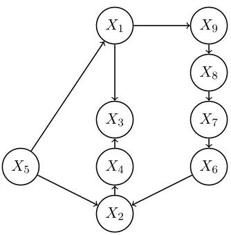
the trek, which is the corresponding coefficient in the SEM. This is shown in full detail by Sullivant et al. (2010), who also show that the covariance conditional on a d-separating set S leaves out treks which include any nodes in S. This conditioning effect is illustrated in Figure 1, where conditioning on an appropriate set S blocks the treks between non-adjacent nodes, without resulting in any additional d-connecting paths. If all edge weights are bounded by 1 in absolute value, then the contribution of each trek to the covariance decays exponentially in trek length. In practice, we scale the data matrix X so that each column has unit standard deviation. Under some conditions, most of the edge weights in the linear SEM (1) then satisfy |ρij|<1 (this is discussed and shown empirically in Appendix
B). Hence, the contribution of long treks to the conditional covariance among non-adjacent nodes is negligible. This decay motivates the thresholding of partial correlations in rPC, and is further discussed in Section 4.
The above observation suggests a new strategy for learning DAG structures by only considering short treks. SupposeS is the set that blocks all short treks between two nodes
j and k. If the correlation over all remaining d-connecting paths (after conditioning on S) between j and k is negligible, then the partial correlation given S, ρ(Xj, Xk | S) can be
used to determine whether j andk are adjacent.
To determine the size of the conditioning set, S, we need to determine the number of short treks between any two nodes j and k. Our second key observation addresses this question, by utilizing properties of large random graphs. More specifically, motivated by Anandkumar et al.’s proposal for estimating undirected graphs, we consider a key feature of large random networks, known as the thelocal separation property.
Definition 6 Given a graph G, aγ-local separator Sγ(i, j)⊂V between non-neighbours i
and j minimally separates iand j with respect to paths of length at mostγ.
Definition 7 A family of graphs G satisfies the (η, γ)-local separation property if, as p →
X1
X2
X3
X4
X5 X6
X7
X8
X9
Figure 1: Illustration of treks between nodes X1 and X2 within a DAG. The middle path involves a collider, X3, so does not contribute to cov(X1, X2), which is ρ51ρ52+
ρ19ρ98ρ87ρ76ρ62 The conditional covariance cov(X1, X2 |X5) excludes treks that involve X5, and is thus ρ19ρ98ρ87ρ76ρ62. Here, S = {X5, X7} is a d-separating set, as it blocks both treks, giving cov(X1, X2|S) = 0.
Intuitively, under (η, γ)-local separation, with high probability, the number of short treks—of length at mostγ—between any two non-neighbouring nodes is bounded above by
η. In fact, as the local separation property refers to any type of path, there are likely even fewer thanη short treks between any two neighbouring nodes. Therefore, we only need to consider conditioning on setsS of size at mostη in order to remove the correlation induced by short treks. Combining this with our first insight, we ignore treks (and other possible d-connecting paths) of length longer thanγ, which, for appropriate probability distributions, have a negligible impact on partial correlations. The resulting procedure, called the full reduced PC-Algorithm (rPC-full), is presented in Algorithm 1.
We note a key implementation difference between rPC-full and the ordinary PC-Algorithm: when searching for a separating set, rPC-full considers allS⊂V\{i, j}, while PC-Algorithm only searches over the local neighbourhoods of iand j. Recall that if a set S d-separates nodesiandj, then there exists a d-separating setS0 such that all nodes inS0 are adjacent to i or j. However, |S0| may be larger than |S|; because rPC only considers sets of size up to η, a full search is needed to ensure discovery of a d-separating set. Motivated by the PC-Algorithm, we also propose an approximate reduced PC-Algorithm (rPC-approx), which uses the same local neighbourhood search, i.e. S ⊂adj(i)∪adj(j)\ {i, j}. In practice, we show that rPC-approx performs almost identically to rPC-full.
graphs, and graphs with power law degree distributions all satisfy this property withη≤2. Moreover, the sparsity requirement for these graph families is in terms of average node degree, and not the maximum node degree. For these graph families, our algorithm only needs to consider separating sets of size 0, 1, and 2, irrespective of the maximum node degree. Small-world graphs, as generated by the Watts-Strogatz algorithm (Kleinberg, 2000), also satisfy this property, but with η > 2. In addition, the γ parameter increases withpfor these families; thus, as graphs get larger, the local separation property applies to a larger set of paths.
By only considering a bounded number of short paths, our algorithm has computational complexityO(pη+2), and thus avoids the exponential scaling indmaxthat the PC-Algorithm
suffers from. This is particularly significant in the case of power-law graphs, wheredmax=
O(pa) fora >0 (Molloy and Reed, 1995); in this case, PC-Algorithm has a computational complexity of O(ppa), which is significantly worse than rPC’s complexity of O(p4). While rPC-full might not be faster in practice due to the larger search space, rPC-approx would result in significant speedup.
Unlike the first property (P1), the second property needed for our algorithm, namely the negligibility of correlation over d-connecting paths, concerns both the structure of the DAGG, and the probability distribution P of variables on the graph. In the next section, we discuss two alternative sufficient conditions that guarantee this property, and allow us to consistently estimate the DAG skeleton.
INPUT: Observations from random variablesX1, X2, . . . , Xp; threshold levelα;
maximum separating set sizeη. OUTPUT: Estimated skeleton C.
SetV ={1, . . . , p}.
Form the complete undirected graph ˜C on the vertex setV. Setl=−1;C= ˜C.
repeat
l=l+ 1
repeat
Select a (new) ordered pair of nodes i, j that are adjacent inC
repeat
Choose (new)S⊂V \ {i, j} with|S|=l
if ρ(Xi, Xj |S)≤α
Delete edge (i, j)
Denote this new graph by C
end if
untiledge (i, j) deleted or allS⊂V \ {i, j}with |S|=lhave been chosen
until all ordered pairs of adjacent nodesiand j have been examined for ρ(Xi, Xj |S)≤α
untill > η
4. Algorithm Analysis and Asymptotics
In this section, we describe in detail the assumptions required for the rPC-full algorithm to consistently recover the DAG skeleton. We also discuss its computational and statistical properties, particularly in comparison with the PC-Algorithm.
4.1. Consistency
As discussed in the previous section, to consistently recover the DAG skeleton, rPC re-quires that properties (P1) and (P2) hold; namely, that the graph under consideration has a bounded number of short paths and the correlation over d-connecting paths of length greater thanγ decays sufficiently quickly. In fact, the trek decomposition (2) indicates that the correlation for each long trek is small when most of the edge weights are bounded by 1 in absolute value. However, condition (P2) requires the total correlation over all long treks (and other d-connecting paths) to decay sufficiently quickly. To this end, we con-sider two alternative sufficient conditions. The first condition is a direct assumption on the boundedness of the conditional correlation. The second is inspired by Anandkumar et al. (2012), and assumes the underlying probability model satisfies what we termdirected
walk-summability. This condition mirrors the walk-summability condition for undirected
graphical models, which has been well-studied and shown to hold in a large class of models (Malioutov et al., 2006).
Definition 8 A probability model is directed β-walk-summable on a DAG with weighted
adjacency matrixA, ifkAk ≤β <1 where k · k denotes the spectral norm.
As an alternative to this condition, we also present a direct assumption, Assumption 4. This condition is less restrictive than directed walk-summability, but has not been char-acterized in the literature. However, given that γ increases with p in the graph families we are considering, it is intuitive that the sum of edge weight products over treks longer than length γ will be decreasing and asymptotically small. This also holds for non-trek d-connecting paths. These two assumptions lead to two parallel proofs of the consistency of our algorithm, presented in Theorem 1. Before stating the theorem, we discuss our assumptions.
Similar to the PC-Algorithm, our method requires a faithfulness condition. As stated previously, our condition, which we termpath faithfulness and is defined next, is weaker than PC-Algorithm’s λ-strong faithfulness stated in Definition 4 (see Section 4.2 for additional details).
Definition 9 Given λ ∈ (0,1), a distribution P is said to be λ-path-faithful to a DAG
G= (V, E) if both of the following conditions hold:
(i) min{|ρ(Xi, Xj |XS)|: (i, j)∈E, S ⊂V \ {i, j},|S| ≤η}> λ, for some η, and
(ii) min{|ρ(Xi, Xj |XS)|: (i, j, S)∈NG}> λ, where NG is the set of triples (i, j, S) such
that i, j are not adjacent, but there exists k ∈ V making (i, j, k) an unshielded triple, and
i, j are not d-separated given S.
for conditioning sets of size up to dmax. In Section 4.2, we discuss how this affects bounds
on the true partial correlations, and also empirically show that the above path faithfulness assumption is less restrictive than corresponding assumption for the PC-Algorithm.
Assumption 1 (Path faithfulness and Markov property) The probability distribution
P of random variables corresponds to a linear SEM (1) with sub-Gaussian errors, and is
λ-path-faithful to the DAGG, withλ= Ω(n−c) for c∈(0,1/2).
Our second assumption ensures that the covariance matrix of the structural equation model and its inverse remain bounded asp grows.
Assumption 2 (Covariance and precision matrix boundedness) The covariance ma-trix of the modelΣGand its inverseΣ−G1are bounded in spectral norm, that is,max(kΣGk,kΣ−G1k)≤
M <∞ for allp.
The last three assumptions characterize applicable graph families and probability dis-tributions.
Assumption 3 ((η, γ)-local separation) The DAG G belongs to a family of random graphs G that satisfies the (η, γ)-local separation property with η=O(1) and γ =O(logp).
Assumption 4 (Bounded long path weight) Letπdenote a d-connecting path of length
l(π) between two non-adjacent vertices i and j in G. Then, there exists a conditioning set
S such that the total edge weight over d-connecting paths longer than γ satisfies:
p−1 X
l=γ+1 X
l(π)=l
|ρπ,1. . . ρπ,l|=O(βγ),
for some β ∈(0,1).
Assumption 4 guarantees that the sum of weights over long treks between any two nodesi
andjis bounded. For a single trek, a sufficient condition is that all edge weights are bounded by 1 in magnitude. In Appendix B, we provide further discussion on Assumption 4, and empirically investigate its plausibility. In particular, we show that if the data matrixX is scaled so that each column has unit standard deviation, then with high probability all edge weights are bounded by 1 in absolute value. To account for residual correlation induced through conditioning on common descendants ofiand j, Assumption 4 also includes non-trek d-connecting paths.
Assumption 40 (Directed β-walk-summability) The probability distribution P is
di-rected β-walk-summable.
We are now ready to state our main result. The result is proved in Appendix A, where the error probabilities are also analyzed.
Theorem 1 Under Assumptions 1-3 and either Assumption 4 or 40, there exists a parame-terαfor thresholding partial correlations such that, asn, p−→ ∞withn= Ω{(logp)1/(1−2c)}, the full reduced PC (rPC-full) procedure, as described in Algorithm 1, consistently learns
Several theoretical features of our algorithm are attractive. As stated previously, our faithfulness condition is weaker than the corresponding assumption for the PC-Algorithm and related methods. Similar to its computational complexity, the sample complexity of our algorithm also does not scale with the maximal node degree, and is only dependent on the parameterη as pincreases. For example, in a power law graph, the sample complexity of the PC-Algorithm is Ω{max(logp, pab)} for 0 < a, b < 1, compared to Ω{(logp)1/1−2c}
with c∈(0,1/2) for our method. This gain in efficiency is due to fact that the maximum separating set size, η, remains constant in rPC. Finally, our algorithm does not require the data to be jointly Gaussian. The proof of the algorithm’s consistency only requires that the population covariance matrix can be well-approximated from the data; for simplicity, we assume a sub-Gaussian distribution.
4.2. On Faithfulness Assumption
As stated in Section 2.2, for large biological networks of interest, the maximum node degree,
dmax, often grows withp. Therefore, theλ-restricted strong faithfulness condition of the
PC-Algorithm—Definition 4—becomes exponentially harder to satisfy with increasing network size. A full discussion of this phenomenon can be found in Uhler et al. (2013), where it is shown that the measure of strong unfaithful distributions converges to 1 for various graph structures. Although this would also occur with path faithfulness (Definition 9), our condition allows a rate for λthat is independent ofdmax and p.
The rate for λ in the PC-Algorithm is λ = Ω(n−w) for w ∈ (0, b/2), where dmax =
O(n1−b) forb∈(0,1]. Forb= 1, or constantd
max, the PC-Algorithm’s required scaling for
λis identical to that for our method in Assumption 1. This makes sense intuitively, since our method is not affected by the increase indmax. For other values of b, the scaling of λ
becomes more restricted for the PC-Algorithm; for example, if b = 1/2, then λ= Ω(n−w) forw∈(0,1/4). However, under path faithfulness (Definition 9), we can still achieve a rate ofλ= Ω(n−1/2); that is, the partial correlations are allowed to be smaller and the condition is weaker.
We report the findings of a simulation study, similar to that in Uhler et al. (2013), which examines how often randomly generated DAGs satisfy part (i) of the path faithfulness assumption compared to restricted strong faithfulness. We are primarily interested in part (i), as this part is needed for consistent skeleton estimation; part (ii), on the other hand, is needed to obtain correct separating sets in order to obtain partial orientation of edges. In this simulation, 1000 random DAGs were generated from Erd˝os-R´enyi and power law families, with edge weights drawn independently from a Uniform(−1,1) distribution. Each DAG had p = 20 nodes, with varying expected degrees per node. For each simulation setting, we computed the proportion of DAGs that satisfied part (i) of the λ -restricted-strong-faithfulness and λ-path-faithfulness conditions with λ = 0.001 and η = 2. The results are shown in Table 1. We see that path faithfulness is much more likely to be satisfied than restricted strong faithfulness, especially for power law graphs. This is to be expected, as the number of constraints required for restricted strong faithfulness grows with
dmax, but remains constant for path faithfulness. It is, however, difficult for dense graphs
Graph family Expected degree P r(RSF) P r(PF) Erd˝os-R´enyi 2 0.77 0.92
Erd˝os-R´enyi 5 0 0.08
Power law 2 0.54 0.85
Power law 6 0.003 0.08
Table 1: Empirical probabilities of random DAGs of size p = 20 satisfying faithfulness conditions; RSF refers to restricted strong faithfulness of the PC-Algorithm, and PF refers to path faithfulness of reduced PC (rPC).
both of these give similar conclusions and indicate that path faithfulness remains easier to satisfy with increasing network size.
4.3. Tuning Parameter Selection
Our algorithm requires two tuning parameters: the maximum separating set sizeη, and the threshold level for partial correlations α. The parameterη varies based on the underlying graph family. Thus, given knowledge of a plausible graph structure,η can be pre-specified. Alternatively,ηcan be selected by maximizing a goodness-of-fit score over a parameter grid, along withα. This may be preferable as the local separation results consider all short paths, not just treks, so better performance may be obtained by specifying a smaller η. Likewise, when using the rPC-approx algorithm, a larger η could be needed to discover appropriate separating sets.
For jointly Gaussian data, we can obtain a modified version of the Bayesian information criterion by fitting the likelihood to the CPDAG obtained based on the estimated DAG skeleton (Foygel and Drton, 2010). Following Anandkumar et al. (2012), and denoting by
Xobs the observed data, we use:
bic(Xobs; ˆG) = logf(Xobs; ˆθ)−0.5|E|log(n)−2|E|log(p), (3)
where ˆG denotes one of the DAGs obtained from the estimated CPDAG containing |E|
edges. The CPDAG represents the Markov equivalence class of DAGs, so all possible graphs will result in the same fitted Gaussian model with parameters ˆθ. We use thisbicfor tuning
parameter selection; higher scores imply a better fit. For linear SEMs with non-Gaussian noise distributions, the Gaussian likelihood serves as a surrogate goodness-of-fit measure, and biccan still be used to select the tuning parameters.
5. Simulation Studies
0.00 0.02 0.04
0.0
0.2
0.4
0.6
0.8
1.0
False positive rate
T
rue positiv
e r
ate
0.00 0.02 0.04
0.0
0.2
0.4
0.6
0.8
1.0
False positive rate
T
rue positiv
e r
ate
0.00 0.02 0.04
0.0
0.2
0.4
0.6
0.8
1.0
False positive rate
T
rue positiv
e r
ate
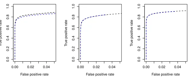
Figure 2: Average true vs. false positive rates for PC-Algorithm (grey solid line), rPC-approx (black dashed line), and rPC-full (blue dashed line) estimating Erd˝ os-R´enyi DAGs. Left: p = 100, n = 200; centre: p = 200, n = 100; right: p = 500, n= 200.
5.1. Pre-specified η Parameter
To facilitate the comparison with the PC-Algorithm, we generate data from Gaussian linear SEMs as in Equation 1, with the dependency structure specified by a DAG from Erd˝ os-R´enyi and power law families. We implement our algorithm with maximum separating set size η = 2 since these families are known to satisfy (η, γ)-local-separation with η ≤ 2 (Anandkumar et al., 2012).
We generate a random graph with p nodes using the igraph library in R, assigning every edge a weight from a Uniform(0.1,1) distribution. We then use the rmvDAGfunction from thepcalglibrary to simulatenobservations from the DAG. This is repeated 20 times for each thresholding levelα; average true and false positive rates for both algorithms are reported over the grid ofα values. Our grid ofαvalues produces partial receiver operating characteristic (pROC) curves for varying sample sizes and graph structures, which are used to assess the estimation accuracy of the methods.
For both Erd˝os-R´enyi and power law DAGs, we consider a low-dimensional setting with p = 100 nodes and n = 200 observations, and two high-dimensional settings with (p, n) = (200,100) and (p, n) = (500,200). In all settings, the DAGs are set to have an average degree of 2. The maximum degrees of the Erd˝os-R´enyi graphs range from 5 to 7. The maximum degrees for power law graphs increase withp and are 42, 69, and 71 for the three simulation settings.
Results for Erd˝os-R´enyi DAGs are shown in Figure 2. In this setting, all algorithms perform almost identically in both low and high-dimensional cases. This is because for the relatively small maximum degree in Erd˝os-R´enyi graphs, the sizes of conditioning sets for PC and rPC are not very different.
0.00 0.02 0.04 0.0 0.2 0.4 0.6 0.8 1.0
False positive rate
T
rue positiv
e r
ate
0.00 0.02 0.04
0.0 0.2 0.4 0.6 0.8 1.0
False positive rate
T
rue positiv
e r
ate
0.00 0.02 0.04
0.0 0.2 0.4 0.6 0.8 1.0
False positive rate
T
rue positiv
e r
ate
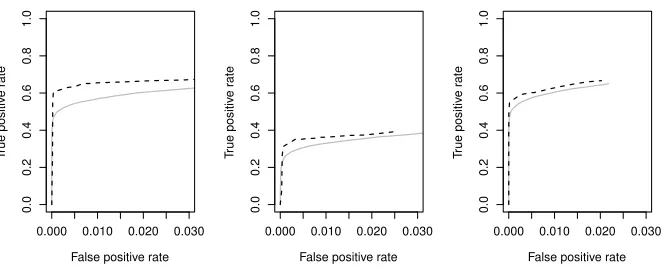
Figure 3: Average true vs. false positive rates for PC-Algorithm (grey solid line), rPC-approx (black dashed line), and rPC-full (blue dashed line) estimating power law DAGs. Left: p= 100, n= 200; centre: p= 200, n= 100; right: p= 500, n= 200.
0.000 0.010 0.020 0.030
0.0 0.2 0.4 0.6 0.8 1.0
False positive rate
T
rue positiv
e r
ate
0.000 0.010 0.020 0.030
0.0 0.2 0.4 0.6 0.8 1.0
False positive rate
T
rue positiv
e r
ate
0.000 0.010 0.020 0.030
0.0 0.2 0.4 0.6 0.8 1.0
False positive rate
T
rue positiv
e r
ate
Figure 4: Average true vs. false positive rates for PC-Algorithm (grey solid line) and rPC-approx withbic-tuned η (black dashed line) estimating power law DAGs. Left:
settings. These results confirm our theoretical findings, and show that our algorithm per-forms better at estimating DAGs with hub nodes than the PC-Algorithm.
Additional simulations in Appendix B show similar results in more dense DAGs. As the underlying DAG becomes more dense, all methods perform worse; however, our algorithms maintain an advantage over the PC-Algorithm in the power law setting. All of these sim-ulations also confirm that rPC-full and rPC-approx perform very similarly. This suggests that the situation where conditioning on non-local sets is required occurs with very low probability, indicating that rPC-approx provides suitably good estimates.
We also compare the runtimes of the algorithms for these settings. Over 100 iterations, we generate a random data set, and apply all the algorithms with a range of tuning param-eters. Specifically, we setη = 2 for rPC, andα =
10−6,10−5,10−4,10−3,10−2 . We then take the total runtime over all parameters, and compare by considering the mean value of 100timerP C
timeP C
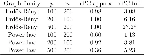
for both rPC-approx and rPC-full. The results are shown in Table 2. We observe that rPC-approx is significantly faster than the PC-Algorithm for power law graphs. As expected, our implementation of rPC-full is slower than the PC-Algorithm in all settings, given its exhaustive search over all possible separating sets. Given the results indicating that rPC-approx performs almost identically to rPC-full, we suggest that practitioners use rPC-approx, possibly combined with bic tuning if a suitable η bound is not known. We
present relevant simulation results in the next section.
Graph family p n rPC-approx rPC-full Erd˝os-R´enyi 100 200 0.98 3.08 Erd˝os-R´enyi 200 100 1.00 6.16 Erd˝os-R´enyi 500 200 1.00 23.25
Power law 100 200 0.60 1.13 Power law 200 100 0.92 3.81 Power law 500 200 0.36 5.23
Table 2: Empirical ratio of rPC-approx and rPC-full runtimes to PC-Algorithm runtime.
5.2. BIC-tuned η Parameter
In this section, we consider simulations where the maximum size of the conditioning set for rPC-approx,η, is selected to maximize thebicscore defined in (3). To this end, we consider
power law DAGs with the same low and high-dimensional settings as before. We select the value ofη∈ {1,2,3,4} which maximizes thebicat eachα value. While rPC-full could also
be tuned in this way, it would be computationally expensive to consider η beyond 3 for
p >200. The results in Figure 4 show that our algorithm maintains an advantage over the
6. Application: Estimation of Gene Regulatory Networks
We apply our algorithms and the PC-Algorithm to a gene expression data set of n = 487 patients with prostate cancer from The Cancer Genome Atlas (Cancer Genome Atlas Research Network, 2012). We select p = 272 genes with known network structure from BioGRID (Stark et al., 2006), and attempt to recover this network from the data. We choose the tuning parameters for both rPC algorithms and the p-value threshold for the PC-Algorithm by searching over a grid of values and selecting those which yielded the largest bic (3). We found that the best rPC algorithm in terms of bic was rPC-approx
withη = 3 andα= 0.09, while the best p-value threshold for the PC-Algorithm was 0.07. The BioGRID database provides valuable information about known gene regulatory interactions. However, this databse mainly capture genetic interactions in normal cells. Thus, the information from BioGRID may not correctly capture interactions in cancerous cells, which are of interest in our application (Ideker and Krogan, 2012). Despite this limitation, highly connected hub genes in the BioGRID network, which usually correspond to transcription factors, are expected to stay highly connected in cancer cells. Therefore, to evaluate the performance of the two methods, we focus here on the identification of hub genes, which are often most clinically relevant (Horvath et al., 2006; Jeong et al., 2001; Carlson et al., 2006).
The two estimated networks and their hub genes are visualized in Figure 5. Here, we define hub genes as nodes with degree at least 8, which corresponds to the 75th percentile in the degree distribution of both estimates. rPC-approx identifies 19 of 57 true hubs, while the PC-Algorithm only identifies 6. Interestingly, several of the hub genes uniquely identified by rPC are known to be associated with prostate cancer, including ACP1, ARHGEF12, CDH1, EGFR, and PLXNB1 (Ruela-de Sousa et al., 2016; Robbins et al., 2011; Ratz et al., 2017; Sun et al., 2017; Liu et al., 2017). These results suggest that rPC may be a promising alternative for estimating biological networks, where highly-connected nodes are of clinical importance.
Examining the two networks also indicates that for nodes with small degrees, the es-timated neighborhoods from rPC are very similar to those from the PC-Algorithm. To assess this observation, we consider the induced subgraph of nodes with degree at most 5 in the PC-Algorithm estimate. TheF1 score—which is a weighted average of precision and recall—between the two estimates of this sparse subnetwork is 0·86. This value indicates that the two algorithms perform very similarly over sparse nodes.
7. Discussion
Figure 5: Estimated skeletons of gene regulatory networks in prostate cancer subjects. Black nodes are classified as hubs, having estimated degree of at least 8. Grey nodes are identified hubs that are also considered hubs in the BioGRID data. Left: PC-Algorithm; right: rPC-approx.
on small sets of variables can also be used to develop more efficient hybrid methods for learning DAGs in high dimensions.
Acknowledgments
Appendix A. Proof of Theorem 1
In this section, we prove the consistency of rPC-full for estimating the skeleton of a directed acyclic graph under the assumptions stated in the main paper.
We begin by establishing that correlations decay over long paths in the graph, and use this to show that the partial correlation between two non-adjacent nodes, conditional on a suitable set S with small cardinality, is bounded above. We establish this through two possible sufficient conditions: Lemma 1 is based on Assumption 4, which directly assumes that the the total weight over long paths is sufficiently small; on the other hand, Lemma 2 uses Assumption 40, which assumes the underlying model is directed walk-summable. Combining this result with Assumption 1, which says that the relevant partial correlations between two adjacent nodes is bounded below, we have oracle consistency of rPC-full. In Lemma 3, we invoke a concentration inequality for sample partial correlations to bound their deviations from population quantities. Using these results, we then prove that there ex-ists a threshold level that consistently recovers the true skeleton in the finite sample setting.
In our first two lemmas, we make use of the local separation property in Assumption 3. While Assumption 3 does not directly concern local separating sets, since a d-separating set is a subset of a general separating set, Assumption 3 asymptotically guarantees the existence of a γ-local d-separator of size at mostη for any two non-neighbouring nodes.
Definition 10 Given a graph G, a γ-local d-separator Sγ(i, j) ⊂ V \ {i, j} between
non-neighbours iand j minimally d-separatesi and j over paths of length at most γ.
Lemma 11 Under Assumptions 1-4, the partial correlation between non-neighbours i and j satisfies
min
S∈Sη,γ
|ρ(i, j|S)|=O(βγ).
where Sη,γ is the set of γ-local d-separators of size at most η.
Proof
Recall the form of the linear structural equation model:
Xk=
X
j∈pa(k)
ρjkXj+k,
wherek are independent and V ar(k) =σ2k<∞ for all k.
LetAGdenote the lower-triangular weighted adjacency matrix for the graphG, obtained
by ordering the nodes according to a causal order (Shojaie and Michailidis, 2010), so that
j∈pa(k) impliesj < k. Then, as shown by Shojaie and Michailidis (2010) for the Gaussian case and by Loh and B¨uhlmann (2014) in general linear structural equation models,
ΣG= (I−AG)−1D(I−AG)−T,
whereD= diag(σ21, ..., σp2).
First, suppose that σi2= 1 for all i. We consider the conditional covariance ΣG(i, j |S)
π denote a d-connecting path between i and j of length l(π), and ρ1, . . . , ρl denote the
edge weights along the path. By conditioning onS, we have that covariance is only induced through d-connecting paths of length greater thanγ, as referenced in the main paper. Then,
ΣG(i, j|S) =
X
π:i↔j π∩S=∅
X
π:l(π)=l l
Y
k=1
ρk=
p−1 X
π:i↔j l(π)=γ+1
X
π:l(π)=l l
Y
k=1
ρk.
Therefore:
|ΣG(i, j|S)|=
p−1 X
π:i↔j l(π)=γ+1
X
π:l(π)=l l Y k=1 ρk ≤
p−1 X
π:i↔j l(π)=γ+1
X
π:l(π)=l l
Y
k=1
|ρk| (by triangle inequality)
=O(βγ). (by Assumption 4)
Now, suppose that not all σi2 = 1. Then, letσmax2 = maxiσi2. We have:
|ΣG(i, j|S)| ≤ p−1 X
π:i↔j l(π)=γ+1
X
π:l(π)=l
σmax2
l
Y
k=1
|ρk|
=σmax2
p−1 X
π:i↔j l(π)=γ+1
X
π:l(π)=l l
Y
k=1
|ρk|
=σmax2 O(βγ)
=O(βγ). (by Assumption 2)
Finally, we have |ρ(i, j | S)| = p |ΣG(i, j|S)|
ΣG(i, i|S)ΣG(j, j|S)
= O(βγ) by Assumption 2,
since the conditional variances are functions of the marginal variances, which are bounded.
Next, we show the same result by assuming directed walk-summability of the model.
Lemma 12 Under Assumptions 1-3 and Assumption 40, the partial correlation between
non-neighbours iand j satisfies
min
S∈Sη,γ
|ρ(i, j|S)|=O(βγ).
Proof
Recall from the proof of Lemma 1,
ΣG= (I−AG)−1D(I−AG)−T,
whereD= diag(σ21, ..., σp2). First, suppose thatσ2i = 1 for all i. Then, we can write:
ΣG=
∞ X
r=0
ArG
! ∞ X
r=0
ArG
!T = γ X r=0
ArG+
∞ X
r=γ+1
ArG
γ X r=0
ArG+
∞ X
r=γ+1
ArG
T
.
Now, let ΣH denote the covariance matrix induced by only considering d-connecting
paths of length at most γ. For convenience, let ΛH := Pγr=0ArG and Rγ := P∞r=γ+1ArG.
Considering their spectral norms, denoted by k · k, we have by walk-summability that
kΛHk ≤
1−βγ+1
1−β and kRγk ≤
βγ+1
1−β. Then,
ΣG= (ΛH +Rγ)(ΛH+Rγ)T
= ΛHΛTH + ΛHRTγ +RγΛTH +RγRTγ
= ΣH + ΛHRTγ +RγΛTH +RγRTγ
Now, defining Eγ := ΣG−ΣH and taking spectral norms, we get:
kEγk=kΣG−ΣHk=kΛHRTγ +RγΛTH+RγRTγk
≤ kΛHRTγk+kRγΛTHk+kRγRTγk
≤2kΛHkkRγk+kRγk2
≤2
1−βγ+1 1−β
βγ+1
1−β
+
βγ+1
1−β
2
= 2β
γ+1−2β2γ+2 (1−β)2 +
β2γ+2
(1−β)2 = 2β
γ+1−β2γ+2 (1−β)2 = β
γ+1(2−βγ+1) (1−β)2
=O(βγ). (S1)
Now, suppose that not all σi2= 1. Then, following the same expansion of ΣG as above,
we have:
kEγk=kDk
βγ+1(2−βγ+1)
(1−β)2 =σ 2
max
βγ+1(2−βγ+1)
(1−β)2 =O(β
by Assumption 2, where σmax2 = maxiσ2i.
We now show that |ρ(i, j | S)| = O(kEγk) = O(βγ) where S is a γ-local d-separator
betweeniandj. LetA={i, j} ∪S andB=V\A. Consider the marginal precision matrix,
P :={ΣG(A, A)}−1. Then, using the Schur complement, we can write this as
P = Σ−G1(A, A)−Σ−G1(A, B){Σ−G1(B, B)}−1Σ−G1(B, A).
Specifically, the partial correlation ofXiandXjconditional onSis given by(P P1,2
1,1P2,2)1/2 =
O(P1,2), by Assumption 2.
Recall from (S1) that ΣG = ΣH+Eγ. LetFγ be the matrix such that ΣG−1 = Σ−H1+Fγ.
Because ΣH only considers covariance induced by paths of length at most γ, we have that
Σ−H1(A, A)1,2 = 0. Thus,
|{ΣG(A, A)}−1,12|=|Σ −1
G (A, A)1,2−Σ−G1(A, B){Σ
−1
G (B, B)}
−1Σ−1
G (B, A)1,2|
=|Σ−H1(A, A)1,2+Fγ(A, A)1,2−ΣG−1(A, B){Σ−G1(B, B)}−1Σ−G1(B, A)1,2| =|Fγ(A, A)1,2−Σ−G1(A, B){ΣG−1(B, B)}−1ΣG−1(B, A)1,2|
≤ kFγ(A, A)−Σ−G1(A, B){ΣG−1(B, B)}−1Σ−G1(B, A)k∞
≤ kFγ(A, A)−Σ−G1(A, B){ΣG−1(B, B)}−1Σ−G1(B, A)k.
However, since ΣG−1(A, B){ΣG−1(B, B)}−1Σ−1
G (B, A) is positive semi-definite,|{ΣG(A, A)}
−1 1,2| ≤
kFγ(A, A)k. We next show that kFγk=O(kEγk) =O(βγ). First, note that:
Fγ = Σ−G1−Σ−H1
= (ΣH +Eγ)−1−Σ−H1
= ΣH−1−Σ−H1(Eγ−1+ ΣH−1)−1Σ−H1−Σ−H1 (by Woodbury) =−Σ−H1(Eγ−1+ Σ−H1)−1Σ−H1
Then, taking spectral norms, and noting that ΣG = ΣH+Eγ:
kFγk ≤ kΣ−H1kk(E−γ1+ Σ−H1)
−1kkΣ−1
H k (by sub-multiplicity)
=kΣ−H1k2kE
γ−Eγ(ΣH +Eγ)−1Eγk (by Woodbury)
=kΣ−H1k2kEγ(I−Σ−G1Eγ)k
≤ kΣ−H1k2kEγkkI−Σ−G1Eγk (by sub-multiplicity)
≤ kΣ−H1k2kE
γk(1 +kΣ−G1Eγk) (by triangle inequality)
≤ kΣ−H1k2kEγk(1 +kΣ−G1kkEγk) (by sub-multiplicity)
≤JkEγk2, (by boundedness of kΣ−G1k ≥ |Σ−H1k)
for some constant J. Then, by walk-summability, kFγk = O(|Eγk). Hence, |ρ(i, j |
By combining the result from either Lemma 1 or 2 with theλ-path-faithfulness assump-tion, we achieve oracle consistency for our algorithm given a threshold level α such that
α=O(λ), α= Ω(βγ).
Next, we consider the finite sample setting, and establish a concentration inequality for sample partial correlations, under sub-Gaussian distributions, using a result from Raviku-mar et al. (2011).
Lemma 13 AssumeX = (X1, ..., Xp)is a zero-mean random vector with covariance matrix
Σ such that each Xi/Σii1/2 is sub-Gaussian with parameter σ. Assume kΣk∞ and σ are
bounded. Then, the empirical partial correlation obtained from n samples satisfies, for some bounded M >0:
P
max
i6=j,|S|≤η
|ρˆ(i, j|S)−ρ(i, j|S)|>
≤4
3 +3 2η+
1 2η
2
pη+2exp
−n
2
M
for all ≤maxi(Σii)8(1 + 4σ2).
Proof
Using the recursive formula for partial correlation, for any k∈S
ρ(i, j |S) = ρ(i, j|S\k)−ρ(i, k|S\k)ρ(k, j|S\k)
(1−ρ2(i, k |S\k))1/2(1−ρ2(k, j |S\k))1/2. For example, with S={k}, we can simplify this to:
ρ(i, j|S) = ρ(i, j)−ρ(i, k)ρ(k, j)
(1−ρ2(i, k))1/2(1−ρ2(k, j))1/2, whereρ(i, j) = Σij/(ΣiiΣjj)1/2.
Rewriting in terms of elements of Σ, we then decompose the empirical partial correlation deviance from the true partial correlation into the deviances of covariance terms. Here, the event of the empirical partial correlation being within distance of the true partial correlation is contained in the union of the empirical covariance terms being within C
distance of the true covariance terms for a sufficiently largeC >0:
|ρˆ(i, j|S)−ρ(i, j |S)|>
⊂
|Σˆij −Σij|> C
[
|Σˆii−Σii|> C
[
|Σˆjj−Σjj|> C
[
k∈S
|Σˆik−Σik|> C
[
k∈S
|Σˆjk−Σjk|> C
[
k≤k0∈S
|Σˆkk0−Σkk0|> C
The number of events on the right-hand side is 3 +|S|+|S|+|S|2− |S| 2
. For|S| ≤η, the number of events is then bounded by 3 + 32η+ 12η2. Then, by applying Lemma 1 in Ravikumar et al. (2011), we have that, for anyi, j:
P r
|ρˆ(i, j|S)−ρ(i, j|S)|>
≤4
3 +3 2η+
1 2η 2 exp −n 2 K ,
for someK >0, bounded whenkΣk∞andσ are bounded. From here, the result follows.
Combining the results established in Lemmas 1-3, we now prove the consistency of our algorithm in the finite sample setting.
Let α denote the threshold where if ˆρG(i, j |S) < α, the edge (i, j) is deleted. LetGS
denote the true undirected skeleton ofG, and letSη,γ denote the set ofγ-local d-separators
or size at mostη.
For any (i, j)6∈GS, define the false positive event as
F1(i, j) =
min
S∈Sη,γ
|ρˆG(i, j|S)|> α
.
Define
θmax= max
(i,j)6∈GS min
S∈Sη,γ
|ρG(i, j|S)|
and
ˆ
θmax = max
(i,j)6∈GS min
S∈Sη,γ
|ρˆG(i, j|S)|.
Consider
P r
[
(i,j)6∈GS
F1(i, j)
=P r(ˆθmax> α)
=P r(|θˆmax−θmax|>|α−θmax|)
=O
pη+2exp
−n(α−θmax)
2
M
(by Lemma 3)
whereθmax=O(βγ) by Lemma 1 and 2.
For any true edge (i, j)∈GS, define the false negative event as
F2(i, j) =
min
S⊂V\{i,j},|S|≤η|ρˆG(i, j|S)|< α
.
Define
θmin= min
(i,j)∈GS
min
S⊂V\{i,j},|S|≤η
|ρG(i, j|S)|
and
ˆ
θmin = min
(i,j)∈GS
min
S⊂V\{i,j},|S|≤η
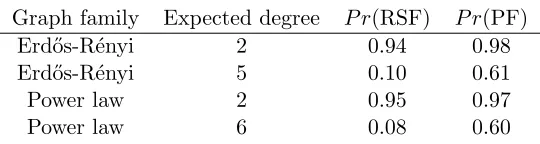
Graph family Expected degree P r(RSF) P r(PF) Erd˝os-R´enyi 2 0.94 0.98 Erd˝os-R´enyi 5 0.10 0.61
Power law 2 0.95 0.97
Power law 6 0.08 0.60
Table 3: Empirical probabilities of random DAGs of size p = 10 satisfying faithfulness conditions; RSF refers to restricted strong faithfulness of the PC-Algorithm, and PF refers to path faithfulness of reduced PC (rPC).
Consider
P r
[
(i,j)∈GS
F2(i, j)
=P r(ˆθmin< α)
=P r(|θmin−θˆmin|>|θmin−α|)
=O
pη+2exp
−n(α−θmin)
2
K
(by Lemma 3)
whereθmin = Ω(λ) by restricted path-faithfulness assumption.
Under our assumptions, we have that n = Ω{(logp)1/1−2c}, and λ = Ω(n−c) with
c∈(0,1/2). Rewriting in terms of λ, we have n= Ω(logλ2p). Then, by selecting α such that
α =O(λ), α = Ω(βγ), we have P r{S
(i,j)6∈GSF1(i, j)} =o(1) and P r{ S
(i,j)∈GSF2(i, j)}=
o(1). This completes the proof of Theorem 1.
Appendix B. Additional Simulation Results
In this section, we present some simulation results comparing our algorithms to the PC-Algorithm in estimating dense graphs. The simulation setup is otherwise identical to that described in the main paper. We consider a low-dimensional setting, with p = 100 and
n= 200, as well as a high-dimensional setting, withp= 200 andn= 100. For Erd˝os-R´enyi graphs, we use a constant edge probability of 0.05, corresponding to an expected degree of 5 for the low-dimensional graph and 10 for the high-dimensional graph. For power law graphs, we use an expected degree of 6 in both graphs.
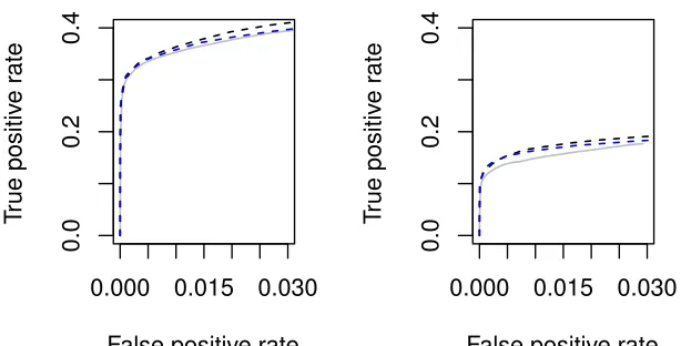
While estimation quality is worse in the dense setting for all methods, we observe in Figure 6 and Figure 7 similar trends as in the main paper. Our methods perform as well as the PC-Algorithm in estimating Erd˝os-R´enyi graphs, and shows some improvement for power law graphs. Both versions of rPC give similar results.
0.000 0.015 0.030
0.0
0.4
0.8
False positive rate
T
rue positiv
e r
ate
0.000 0.006
0.0
0.4
0.8
False positive rate
T
rue positiv
e r
ate
Figure 6: Average true vs. false positive rates for PC-Algorithm (grey solid line), rPC-approx (black dashed line), and rPC-full (blue dashed line) estimating Erd˝ os-R´enyi graphs. Left: p= 100, n= 200, average degree 5; right: p= 200, n= 100, average degree 10.
0.000 0.015 0.030
0.0
0.2
0.4
False positive rate
T
rue positiv
e r
ate
0.000 0.015 0.030
0.0
0.2
0.4
False positive rate
T
rue positiv
e r
ate
Figure 7: Average true vs. false positive rates for PC-Algorithm (grey solid line), rPC-approx (black dashed line), and rPC-full (blue dashed line) estimating power law graphs with average degree 6. Left: p= 100, n= 200; right: p= 200, n= 100.
Graph family Expected degree P r(RSF) P r(PF) Erd˝os-R´enyi 2 0.66 0.86
Erd˝os-R´enyi 5 0 0.01
Power law 2 0.04 0.51
Power law 6 0 0.01
Table 4: Empirical probabilities of random DAGs of size p = 30 satisfying faithfulness conditions; RSF refers to restricted strong faithfulness of the PC-Algorithm, and PF refers to path faithfulness of reduced PC (rPC).
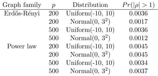
Finally, we consider the plausibility of Assumption 4 when the SEM coefficients are not bounded by 1 in absolute value. Suppose that the data matrix X has been normalized by column-wise standard deviations. We show that this transformation preserves the original network structure, and leads to most edge weights being bounded by 1 in absolute value. Consider an edgej→kand let Wj :={Xi:i∈pa(k)\ {j}}. Then, taking the conditional
covariance:
Cov(Xj, Xk|Wj) =Cov
Xj, ρjkXj +
X
i∈pa(k)\j
ρikXi+k
Wj
=ρjkV ar(Xj|Wj).
We can therefore write:
ρjk =
Cov(Xj, Xk|Wj)
V ar(Xj|Wj)
.
Now, let ˜Xk = Xk/sd(Xk) for all k. Consider the edge weights ˜ρjk corresponding to the
SEM for this transformed data. We have:
˜
ρjk =
sd(Xj)
sd(Xk)
Cov(Xj, Xk|Wj)
V ar(Xj|Wj)
= sd(Xj)
sd(Xk)
ρjk
Clearly, ˜ρjk = 0 if and only ifρjk = 0. Therefore, we recover the same network by applying
our algorithm to the transformed data. Furthermore,
|ρ˜jk|=
s
V ar(Xj)
V ar(Xk)
ρ2
jk
=
v u u t
V ar(Xj)ρ2jk
V ar(Xj)ρ2jk+σk2+Pi∈pa(k)\{j}ρ2ikV ar(Xi) + 2
P
i,i0∈pa(k)ρikρi0kCov(Xi, Xi0) Thus,|ρ˜jk|>1 only if
σ2k+ X
i∈pa(k)\{j}
ρ2ikV ar(Xi) + 2
X
i,i0∈pa(k)
Graph family p Distribution P r(|ρ|>1) Erd˝os-R´enyi 200 Uniform(-10, 10) 0.0036
200 Normal(0, 32) 0.0017 500 Uniform(-10, 10) 0.0036 500 Normal(0, 32) 0.0012 Power law 200 Uniform(-10, 10) 0.0045 200 Normal(0, 32) 0.0045 500 Uniform(-10, 10) 0.0034 500 Normal(0, 32) 0.0037
Table 5: Empirical average probabilities of standardized coefficients exceeding 1 in absolute value.
Rewriting the variance and covariance terms as trek sums, we obtain:
σk2+ X
i∈pa(k)\{j}
ρ2ik X
π:u↔i u∈V\{i}
σw2 Y
ρe∈π
ρ2e+ 2 X
i,i0∈pa(k)
ρikρi0k
X
π:i↔i0
σw
Y
ρe∈π
ρe <0
wherew denotes the source or common node in the trek.
Since the first two terms in this expression will always be positive, |ρ˜jk|>1 only if the
covariance sum is both negative and greater in magnitude than the sum of the first two terms. A term in the covariance sum will be negative if there is an odd number of negative terms in the product, and the entire sum will be negative only if there are a sufficient number of these to make the whole sum negative. Even then, the sum over squared trek products would need to be smaller than the covariance term sum in absolute value. Moreover, even if some |ρ˜jk| > 1, the product over the entire trek may still be less than 1 if most of the
other coefficients along a trek are small. Thus, we may still expect the product over the trek to be small.
References
Silvia Acid and Luis M de Campos. Approximations of causal networks by polytrees: an empirical study. In Advances in Intelligent Computing, pages 149–158. Springer, 1994.
Animashree Anandkumar, Vincent YF Tan, Furong Huang, and Alan S Willsky. High-dimensional Gaussian graphical model selection: walk summability and local separation criterion. Journal of Machine Learning Research, 13(1):2293–2337, 2012.
Cancer Genome Atlas Research Network. Comprehensive genomic characterization of squa-mous cell lung cancers. Nature, 489(7417):519–525, 2012.
Marc RJ Carlson, Bin Zhang, Zixing Fang, Paul S Mischel, Steve Horvath, and Stanley F Nelson. Gene connectivity, function, and sequence conservation: predictions from modu-lar yeast co-expression networks. BMC Genomics, 7(1):40, 2006.
Hao Chen and Burt M Sharp. Content-rich biological network constructed by mining pubmed abstracts. BMC Bioinformatics, 5(1):147, 2004.
David Maxwell Chickering. Learning Bayesian networks is NP-complete. InLearning From Data, pages 121–130. Springer, 1996.
Richard Durrett.Random Graph Dynamics, volume 200. Cambridge University Press, 2007.
Daniel Eaton and Kevin Murphy. Bayesian structure learning using dynamic programming and MCMC. arXiv preprint arXiv:1206.5247, 2012.
Rina Foygel and Mathias Drton. Extended Bayesian information criteria for Gaussian graphical models. In Neural Information Processing Systems (NeurIPS), pages 604–612, 2010.
Nir Friedman, Michal Linial, and Iftach Nachman. Using Bayesian networks to analyze expression data. Journal of Computational Biology, 7:601–620, 2000.
Min Jin Ha, Wei Sun, and Jichun Xie. PenPC: a two-step approach to estimate the skeletons of high-dimensional directed acyclic graphs. Biometrics, 72(1):146–155, 2016.
S Horvath, B Zhang, M Carlson, KV Lu, S Zhu, RM Felciano, MF Laurance, W Zhao, S Qi, Z Chen, et al. Analysis of oncogenic signaling networks in glioblastoma identifies aspm as a molecular target. Proceedings of the National Academy of Sciences, 103(46): 17402–17407, 2006.
Juan F. Huete and Luis M. Campos. Learning causal polytrees. In Symbolic and
Quan-titative Approaches to Reasoning and Uncertainty, pages 180–185. Springer, 1993. doi:
10.1007/BFb0028199.
Ronald Jansen, Haiyuan Yu, Dov Greenbaum, Yuval Kluger, Nevan J. Krogan, Sam-bath Chung, Andrew Emili, Michael Snyder, Jack F. Greenblatt, and Mark Gerstein. A Bayesian networks approach for predicting protein-protein interactions from genomic data. Science, 302(5644):449–453, 2003. ISSN 0036-8075. doi: 10.1126/science.1087361.
Hawoong Jeong, B´alint Tombor, R´eka Albert, Zoltan N Oltvai, and A-L Barab´asi. The large-scale organization of metabolic networks. Nature, 407(6804):651–654, 2000.
Hawoong Jeong, Sean P Mason, A-L Barab´asi, and Zoltan N Oltvai. Lethality and centrality in protein networks. Nature, 411(6833):41–42, 2001.
Markus Kalisch and Peter B¨uhlmann. Estimating high-dimensional directed acyclic graphs with the PC-Algorithm. Journal of Machine Learning Research, 8:613–636, May 2007. ISSN 1532-4435.
Jon Kleinberg. The small-world phenomenon: an algorithmic perspective. InACM
Sympo-sium on Theory of Computing, pages 163–170. ACM, 2000.
Bide Liu, Xiao Gu, Tianbao Huang, Yang Luan, and Xuefei Ding. Identification of tmprss2-erg mechanisms in prostate cancer invasiveness: involvement of mmp-9 and plexin b1.
Oncology Reports, 37(1):201–208, 2017.
Po-Ling Loh and Peter B¨uhlmann. High-dimensional learning of linear causal networks via inverse covariance estimation. Journal of Machine Learning Research, 15(1):3065–3105, 2014.
Dmitry M Malioutov, Jason K Johnson, and Alan S Willsky. Walk-sums and belief prop-agation in Gaussian graphical models. Journal of Machine Learning Research, 7(Oct): 2031–2064, 2006.
Michael Molloy and Bruce Reed. A critical point for random graphs with a given degree sequence. Random Structures & Algorithms, 6(2-3):161–180, 1995.
Preetam Nandy, Alain Hauser, and Marloes H Maathuis. High-dimensional consistency in score-based and hybrid structure learning. arXiv preprint arXiv:1507.02608, 2015.
Jonas Peters, Joris M Mooij, Dominik Janzing, and Bernhard Sch¨olkopf. Causal discovery with continuous additive noise models. Journal of Machine Learning Research, 15:2009– 2053, 2014.
Leonie Ratz, Mark Laible, Lukasz A Kacprzyk, Stephanie M Wittig-Blaich, Yanis Tolstov, Stefan Duensing, Peter Altevogt, Sabine M Klauck, and Holger S¨ultmann. Tmprss2: Erg gene fusion variants induce tgf-β signaling and epithelial to mesenchymal transition in human prostate cancer cells. Oncotarget, 8(15):25115, 2017.
Christiane M Robbins, Waibov A Tembe, Angela Baker, Shripad Sinari, Tracy Y Moses, Stephen Beckstrom-Sternberg, James Beckstrom-Sternberg, Michael Barrett, James Long, Arul Chinnaiyan, et al. Copy number and targeted mutational analysis reveals novel somatic events in metastatic prostate tumors. Genome Research, 21(1):47–55, 2011.
Roberta R Ruela-de Sousa, Elmer Hoekstra, A Marije Hoogland, Karla C Souza Queiroz, Maikel P Peppelenbosch, Andrew P Stubbs, Karin Pelizzaro-Rocha, Geert JLH van Leen-ders, Guido Jenster, Hiroshi Aoyama, et al. Low-molecular-weight protein tyrosine phos-phatase predicts prostate cancer outcome by increasing the metastatic potential.
Euro-pean Urology, 69(4):710–719, 2016.
Eric E Schadt, John Lamb, Xia Yang, Jun Zhu, Steve Edwards, Debraj GuhaThakurta, Solveig K Sieberts, Stephanie Monks, Marc Reitman, Chunsheng Zhang, et al. An in-tegrative genomics approach to infer causal associations between gene expression and disease. Nature Genetics, 37(7):710–717, 2005.
Mark Schmidt, Alexandru Niculescu-Mizil, and Kevin Murphy. Learning graphical model structure using l1-regularization paths. In Association for the Advancement of Artificial
Intelligence (AAAI), volume 7, pages 1278–1283, 2007.
Marco Scutari. Learning Bayesian networks with the bnlearn r package. Journal of
Statis-tical Software, 35(1):1–22, 2010. ISSN 1548-7660. doi: 10.18637/jss.v035.i03.
A. Shojaie, A. Jauhiainen, M. Kallitsis, and G. Michailidis. Inferring Regulatory Networks by Combining Perturbation Screens and Steady State Gene Expression Profiles. PLoS One, 9(2):e82393, 2014.
Ali Shojaie and George Michailidis. Penalized likelihood methods for estimation of sparse high-dimensional directed acyclic graphs. Biometrika, 97(3):519–538, 2010.
P. Spirtes, C. Glymour, and R. Scheines. Causation, Prediction, and Search. MIT press, 2nd edition, 2000.
Chris Stark, Bobby-Joe Breitkreutz, Teresa Reguly, Lorrie Boucher, Ashton Breitkreutz, and Mike Tyers. Biogrid: a general repository for interaction datasets. Nucleic Acids
Research, 34(suppl 1):D535–D539, 2006.
Seth Sullivant, Kelli Talaska, and Jan Draisma. Trek separation for Gaussian graphical models. The Annals of Statistics, pages 1665–1685, 2010.
Liang Sun, Jiaju L¨u, Sentai Ding, Dongbin Bi, Kejia Ding, Zhihong Niu, and Ping Liu. Hcrp1 regulates proliferation, invasion, and drug resistance via egfr signaling in prostate cancer. Biomedicine & Pharmacotherapy, 91:202–207, 2017.
Ioannis Tsamardinos, Laura E Brown, and Constantin F Aliferis. The max-min hill-climbing Bayesian network structure learning algorithm. Machine Learning, 65(1):31–78, 2006.
Arend Voorman, Ali Shojaie, and Daniela Witten. Graph estimation with joint additive models. Biometrika, 101(1):85, 2014.
Changwon Yoo, Vesteinn Thorsson, and Gregory F Cooper. Discovery of causal relationships in a gene-regulation pathway from a mixture of experimental and observational DNA microarray data. InPacific Symposium on Biocomputing, volume 7, pages 498–509, 2002.