A Statistical Learning Model utilized to
validate a well-known market hypothesis of
the moving average “death cross.”
Timothy A. Smith#1, Ethan Borjas,
Embry Riddle Aeronautical University
600 S. Clyde Morris Blvd. Daytona Beach, Fl 32114 U.S.A
Abstract — In finance, regression models have been frequently utilized to predict the value of an asset based on its underlying traits. From a prior work a regression model was built to predict the value of the S&P 500 based on macroeconomic predictors which were selected through a process of general subjective knowledge followed by model optimization. In the present work the method of statistical machine learning is utilized to instead decide what predictors are to be used within the model. In addition, a well-known market hypothesis “the 5 year moving average death cross” is mathematical validated, and a scheme to relate those critical time periods to particular values of the regression predictors is outlined.
Keywords — Partial differential equations, regressions, statistical machine learning, financial mathematics. AMS classification: 35K10
I.INTRODUCTION
During the time period of the stock market crash of 2008, it was observed that the commonly used stock
market prediction models, such as the famous Black Scholes Stochastic Partial Differential Equation [1]
demonstrated limitation in their ability to predict during rapidly changing times of volatility [2-3]. As it is well
known, the solution of the Black Sholes will accurately predict the fair price of an option from which future
stock values can be extracted. However, during times of rapidly changing volatility the solution becomes
somewhat unstable and most definitely inaccurate to predict the true real world selling value for the fair price of
the option. A major issue is with actually understanding what real world volatility measures can be utilized to
satisfy what it was intended to be in the original work [1] of Fisher Black & Morton Scholes. It is understood
that they were intending σ to model something equivalent to the variance within a probability distribution, but it
is not so obvious as how to obtain such a value from a real world stock or market index. In recent times many
people have utilized the so called “classical definition of volatility” for σ. Furthermore, in more modern times
many people have utilized the so called “implied definition of volatility” for σ, and of course research continues
recent papers [4-5], a method was informally proposed to define volatility as a measure of how far from the
linear regression model the stock value currently is; hence, defining σ to measure how far the “market” is
actually off from the “economy.” In the present study, we expand this research and also improve the core model
utilized by introducing a statistical learning technique. In theory, this mathematical logic could be applied to
identify market bottom turning points for general stock market indices, such as the S&P 500.
II.INITIALSTATISTICALREGRESSIONMODEL
Various economic indicators allow predictions of the future performance of an economy to be drawn.
In a prior study [4] a number of predictor variables ( AKA major market “drivers” or “indicators” ) were
inputted into a regression analysis. The variables were initially selected by a subjective process - relying on
expertise and common sense along with some existing [6] real world modelling - as to what factors are
commonly thought of to drive the market. Then after routine remodelling and variable removal, by analysing
VIF values and predictor variable’s test stat values, three major indicators were found to be the core model. This
data was utilized to build a multiple variable linear regression model, namely the predictor variables utilized
were the unemployment rate (UI), the gross domestic product (GDP), and the monetary supply (M1) all
measured monthly. The model was found to work quite well with a coefficient of determination well above 0.9.
With publically available data, which is available upon request, a MLR model was constructed from January
1990 to July 2013 of the form
0 1 1 2 2 3 3
y
x
x
x
which yielded the results
Coefficients
Standard
Error t Stat
Intercept 965.0635 6.659789 144.909
GDP 362.1807 28.36177 12.77003
MS 183.392 28.53035 6.427962
UI -173.762 7.021221 -24.7482
ANOVA
df MS F
Regression 3 41499537 2333.34
Residual 397 17785.47
Total 400
It was very surprising to the authors, and many colleagues, that the so called Fed Funds Interest Rate
was not being included in the model. Thus, in our current study the data analysis was rerun on a subjective
process to simply add the variable of Fed Funds Interest Rate ( FFR ) back in as a predictor. After doing so, the
following was obtained
Coefficients t Stat
Intercept 965.0635 144.8561
GDP 349.0002 10.77223
FFR -12.1984 -0.84265
MS 186.5665 6.480629
UI -177.406 -21.5083
ANOVA
df MS F
Regression 4 31127812 1748.904
Residual 396 17798.47
Total 400
Fig. 2 The data analysis of the 4 variable model .
It is observed that both this new model is less significant ( F. Stat of 1748 < 2333 ), and the actual variable of
FFR is not significant itself in the model ( T. Stat of -0.84 < Tα ). Now, if one choses to take a statistically
proper approach, similar to a backwards stepwise regression modelling procedure, they would remove the FFR
variable due to the fact that it does not have a significant test statistic. Thus, a proper approach would be to
revert back to the three variable model
y
i
965.0635
362.1807z + 183.392z
1 3
173.762 .
z
4as previously obtained in Figure 1. Furthermore, not only have we now found a statistical optimal model which,
as one can see above has a very solid F statistic along with R2 value of 0.95, but these results are also quite
interesting as they do show what really drives the market is truly the large macro-economic indicators: the
amount the US produces, the amount of money flowing in the economy and the rate of people unemployed, but
the “common senses” expected predictor of Fed Funds Rate is not included. The point noted here is that the
results should be the truth what the data tells us, not what we subjectively expect! Hence, a good argument to
III.STATISTICALLEARNINGREGRESSIONMODEL
For a more modern approach, with the mass availability of big data, to create a model many additional
predictors could be considered in order to expand our model. Thus, the following scheme is considered which is
preferred for two main reasons: Firstly, and as outlined in the results of the prior section in regards to the
subjectiveness of Fed Funds Rate, it is essential to let the machine along with the data tell us the results as they
will be unbiased unlike our subjectivity. Secondly, the data may change with time and in this modern age of
technology it is a routine exercise to write a python code to constantly be updating our data monthly pulling
from websites API’s or other methods, hence, both the data and the model could be updating in real time. For
example, this can be seen in a quick illustration. If we compare the model outlined in the last section, which had
data [4] from only January 1990 upto July 2013, to an updated rerun of that same model with the most currently
available data (prior to the writing of this article a summer student research project ran the same model with
updated data during the time period upto May of 2019) one would expect the results to differ. This exercise
yielded the results
Coefficients
Standard
Error t Stat
Intercept 975.7634 7.185126 135.8032
GDP 442.7751 22.78631 19.43163
MS 124.956 21.70633 5.756661
UI -186.744 7.053451 -26.4755
ANOVA
df MS F
Regression 3 63306823 2943.593
Residual 421 21506.65
Total 424
Fig. 3 The data analysis of the updated prior 3 variable model.
As these results clearly show this modelling is a very dynamic situation; for example while the structure of MS
and UI within the model did not significantly change, the GDP did. As observed in the old “up to 2013” model
the GDP had a solid coefficient, TS=12, with β coefficient of 362. The fact that it was the most deterministic
predictor variable in the model did not change in the new “up to 2019” model; however, it did both gain a
stronger coefficient, TS = 19, and larger β coefficient of 442. At this point, one may desire to create some sort of
multiple regression model. A desired method would be to utilize an API to pull the most current data monthly
( or perhaps daily, even hourly, if studying individual stocks ) and utilizing data over a shorter time frame,
perhaps the last few years as opposed to several decades as in our prior work. Then one could allow the
computer to define a statistical learning model which is constantly updating itself as time moves on. Hence,
creating a statistical learning model that can change the regression equation, or even possibly what actual
predictors variables are utilized, as time moves forward while keeping the mathematical nature of a routine
regression model as desired.
Now, to develop this scheme we will assume the initial data set is kept with predictors x1,x2, and x3 of our
current working model but many additional data sets are added into the predictor data matrix that “may”
correlate and/or predict the value of the S&P 500 to create a full data vector of X = [x1,x2,x3, x4,x5, … xn ]. To
begin we define the null model
S0
as the model which only contains the intercept, namely
0y
.We then apply a machine learning process to seek the most mathematical pure model with the optimal
set of predictor variables included. Namely, we will construct the first level set of models
{S1}
as the set of n models where each individual model is a simple linear regression model of the form,
0 1 1
y
x
.This single variable model is computed n times separately ( i.e. x1 here is not really our first predictor, rather just
a default label used in standard notation ). Each model individually takes from the predictor data matrix one
column predictor variable, running through 1 to n. Then, for each model the R2 along with the F Statistic is
recorded. Now, at this stage, depending on the number of possible predictor variables available, one may only
want to keep predictor variables that are showing some significance ( a common cut off is to keep a predictor
variable if its R2 > 0.6) to be used for the next level set of models.
We will construct the second level set of models
{S12}
as the set of n*(n-1) models were each individual model is a simple linear regression model of the form
0 1 1 2 2
where the model is computed n*(n-1) times separately. Each model individually takes into the predictor data
matrix only two predictor variable, firstly running through 1 to n through the variable used in S1, then removing
that column from the matrix. Then adding the second variable running through 1 to n-1 through the variables
remaining in the reduced matrix, and this is done for all possible combinations of the two variables. Again for
each model the R2 along with F statistic is recorded.
We then construct the third level set of models
{S123}
as the set of n*(n-1)*(n-2) models were each individual model is a simple linear regression model of the form
0 1 1 2 2 3 3
y
x
x
x
where the model is computed n*(n-1)*(n-2) times separately following the same logical outline as previously
outlined but now for three predictors. And, we then continue this process until the nth level set of models is
obtained as
0 1 1 2 2 n n
y
x
x
x
Now, for each of these models the R2 value along with the F statistic has been recorded, and we desire to find
the best model that is not only mathematically sound ( R2 ), but is also strongly deterministic of our predicted
data ( P value or F Stat ).
After all of the models are computed ( in theory this could be up to 2n models, but it is commonly
significantly less if some predictor variables are discarded after the first level set of models ) the function
23000
L
R
FS
is computed for each model, where the best model will have the highest value of this L function. In purely
mathematical statistical learning model theory at a step like this most researchers would suggest to look at
quantities such as adjusted R2 and/or the Akaike Information Criteria etc, and while those measurements are
very powerful when looking at a pure mathematical error analysis in this research we want to balance that along
with the accuracy described in the F Statistic of the regression model; hence, we use the unique L function
method created above. Further, this function can be thought of similar to a likelihood function in probability
theory, and while in this case the value of 3,000 was chosen by subjective observation ( i.e. from looking at
experimental results F.S values, and if one is applying this logic to a different problem, say for example an
individual stock or sector, they may need to adjust that 3,000 value accordingly ). Furthermore, it could be
constant times R2 then added to FS. However, for our immediate purposes, and from the confidence of prior
research results, the value of 3,000 will suffice. This method now outlines a model that would “learn,” in real
time, which predictor variable’s data is best suited to predict the market with the data given at that time. Also,
the model with the highest L will tell us which predictor variables to use. In a sense, this is a generalization of
the method we outlined in the prior section where the predictor variables which survived are producer price
index (PPI), gross domestic product (GDP), and money supply (M) for our current time frame of data. Also
subjective variables that are not truly deterministic will not survive. Applying this method to that prior data
verifies the result.
IV.APPLICATIONS
The results of our statistical learning model are very far ranging, and many quite practical results, such as
determining market peaks and bottoms, can readily be obtained in real time for either stock market indices or
individual stocks. While we will not cover a large amount of applications here, we will close by quickly
addressing two extremely useful results. Firstly, we will address and expand upon the idea previously mentioned
[4-5] to show how this model can be used to define market volatility. Secondly, we will show a mathematical
validation of the famous hypothesis about the market “death cross” when moving averages intersect, and show
how results from this statistical learning regression model can be utilized to predict such times.
To being, we will revisit some data from the time period around the infamous 2008 stock market crash,
namely the VIX values along with the overall stock market ( S&P 500 ) values. As we can see in this data,
Date
1st of Month SP Opening
VIX
Jan
$1,468
23
Feb
$1,379
24
:
:
:
Oct
$1,164
40
Nov
$969
60
Dec
$889
68
which represents the opening monthly values of the SP 500 index along with the VIX values, during various
months of the infamous 2008 year, the implied volatility ( VIX ) does not foresee the extreme market crash
coming. As if the VIX was truly defining market volatility the values early in the year, or at least mid-year,
would have been spiking rapidly. However, while the VIX did oscillate in the range of high teens to twenties
most of the year, it actually did not grow to value above thirty until Sept 16th ( it is worthy to note here, for the
pure mathematical reader, that generally speaking a value in the tens or lower in the VIX is consider calm, while
values of thirty or higher are considered extremely volatile ). Furthermore, Sept 16th was several days after the
infamous weekend meeting of Fed president Timothy Geithner with Lehmann brothers, which was days prior to
the firms bankruptcy, a key moment of the 2008 crash, perhaps the most volatile time? Now, the point here is
that the VIX index is not a true measure of volatility as Fisher Black and Martin Scholes were intending σ to
model, rather it is a responsive measure as to yesterday’s market. And, likewise are the actual implied volatility
values computed from S&P 500 options real time prices.
In order to create a meaningful measure of volatility the following scheme can be defined. This method
can be computed for various maturity times of options, but for simplification we focus on options with T being
fixed as one year. Now, for a stock with initial value X0, the fair price of the option for this stock can be
computed by the Black Sholes formula
which is the well-known solution of the Black Scholes Stochastic Partial Differential Equation
Here, the commonly utilized notation is k for strike price, r for safe interest rate, σ for volatility, along with N(#)
for the cumulative normal. Now, the question often comes is what exactly is the value “fair price of an option,”
and what can it tell us? In short, the fair price of our T = 1 option would just be how much the stock should
grow in one year, thus if the initial value of the S&P 500 is given as X0 then in one year the value of the S&P
500 value should be X0 + BS, where BS is referring to the output of the Black Sholes formula above. The issue
comes as to what value of σ should be inputted into this formula and results will vary greatly depending on it.
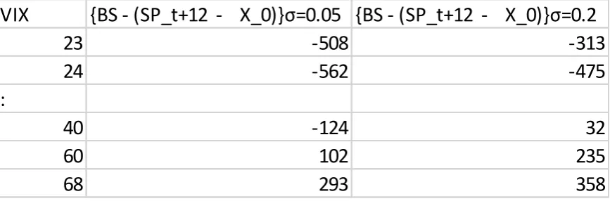
The data set below represents the difference between the predicted value “X0 + BS” of the S&P value 12 moths
VIX
{BS - (SP_t+12 - X_0)}σ=0.05 {BS - (SP_t+12 - X_0)}σ=0.2
23
-508
-313
24
-562
-475
:
40
-124
32
60
102
235
68
293
358
Fig. 5 The data showing a method to better define σ.
As one can see the results vary significantly between the middle column and right column when the volatility is
increased. It is clear that as the volatility is increased the method does improve (for example, in January the
reduction in error is from 508 below to 313 below as volatility increased ), and it is reasonable to believe that if
σ is allowed to continue to increase a value will be obtained where this error becomes 0. Further, if a long term
analysis of this method was computed it would be feasible to define a true value of volatility for past markets.
And, if one had a statistical learning regression model, running on data of that time period, then they could
compare how far of the market was to where the regression model was expecting the market to be. If this was
recorded, in a percentage deviation, this newly complied values of σ they could then define a forward predicting
measure of volatility. Thus, one can say that if Y^ - Y is in a certain range then the value of σ is a certain value,
and then that value of volatility could be inputted into the Black Sholes model. Doing so would lead to
extremely high values of volatility prior to the crash of 2008, and when the Black Sholes model is applied with
such values the results do accurately predict a forthcoming crash. Furthermore, similar results are validated on a
routine analysis of data a few months prior to other large market moves, such as the 2000 dot com crash and the
recent correction of Dec 2018.
V.CONCLUSIONS&DEMONSTRATIONOFMOVINGAVERAGECROSS
In this concluding section, we will end by mathematically validating a well know market hypothesis. Then
we will show how our newly obtained model can be utilized to predict such a market moment forthcoming,
hence concluding with a very practically “real world use” of our research. It has been heavily hypothesized that
when a stock’s short term moving average ( often monthly or 50 day ) falls below its longer term moving
average ( often yearly or longer ) this will lead to a market correction, which we defined here as a 20% or more
Fig. 6 Code used to find 20% market movement times.
was run through the publically available data of S&P 500 values, taken weekly for the last few decades. This
code was designed to find any values where the current value was 20% less than the values of the S&P 500 over
the last year. The values located were noted and compared to a plot of the monthly and 5-year moving average,
and then separately to a plot of the raw stock values. It was verified that these solution values output of the
above code did match up with the crossing points, and at those points corrections were uniquely observed
shortly forward in time (exact timing did vary, as expected).
The statistical learning regression model can be applied to predict these market critical values in terms
of the predictor variables, and this information should be very useful in predictive applications as often changes
to those predictors can be seen earlier. To illustrate this the final values of each variable that we have, May 2019,
were inputted into the equation to then predict a drop of 20% from our predicted value. Namely, the normalized
initial CPI, GDP, UI, along with the stock value of S&P500 values we will use for this exercise are 1.9, 2.299,
-1.7145, and 2952.3 respectfully. This is the true values they were during the summer student’s research project
previously mentioned. At that point in time, the 20% drop of the S&P 500 value can easily be found 2361.864.
Now, it an algebraic exercise to solve for each of the predictors and then put in the values of the other variables
to find the “key values” of each of the predictor variables. For example, if one solve for CPI it yields
For the summer project values these results were individually found for CPI, GDP, and UI to be -2.75, -1.95, an
-0.21 respectively. An improvement on this method could be to correct the other input values, perhaps by
the others doing so to. Regardless of those details these results are very practical real world measures to monitor
and an observation of any of these predictors reaching these critical values could be an indicator of a
forthcoming correction, hence a red light flashing to move to safety.
REFERENCES
[1] Black, F. and Scholes, M. “The Pricing of Options and Corporate Liabilities,” Journal of Political Economy 81 (3), 1973.
[2] Colander, David and Föllmer, Hans and Haas, Armin and Goldberg, Michael D. and Juselius, Katarina and Kirman, Alan and Lux, Thomas and Sloth, Birgitte, “The Financial Crisis and the Systemic Failure of Academic Economics.” Univ. of Copenhagen Dept. of Economics Discussion Paper No. 09-03, 2009
[3] Moyaert, T. & Petitjean, M . “The performance of popular stochastic volatility option pricing models during the subprime crisis.” Applied Financial Economics. 21(14), 2011.
[4] Smith, T. et al, “A Regression Model to Predict Stock Market Mega Movements and/or Volatility using both Macroeconomic indicators & Fed Bank Varaibles.” International Journal of Mathematics Trends and Technology, 49(3), 2017
[5] Smith, T. et al, “Using a Multiple Linear Regression Model to Calculate Stock Market Volatility” International Journal of Mathematic Trends and Technology, 57(4), 2018.