The Thirty-Third AAAI Conference on Artificial Intelligence (AAAI-19)
Exact and Approximate Weighted Model Integration with
Probability Density Functions Using Knowledge Compilation
Pedro Zuidberg Dos Martires, Anton Dries, Luc De Raedt
KU Leuven, BelgiumAbstract
Weighted model counting has recently been extended to weighted model integration, which can be used to solve hybrid probabilistic reasoning problems. Such problems involve both discrete and continuous probability distributions. We show how standard knowledge compilation techniques (to SDDs and d-DNNFs) apply to weighted model integration, and use it in two novel solvers, one exact and one approximate solver. Furthermore, we extend the class of employable weight func-tions to actual probability density funcfunc-tions instead of mere polynomial weight functions.
1
Introduction
The state-of-the-art method for inference in probabilistic graphical models reduces inference to weighted model count-ing (WMC) (Chavira and Darwiche 2008), while utilizcount-ing knowledge compilation (KC) (Darwiche and Marquis 2002). Knowledge compilation transforms the logical structure un-derlying a graphical model into an equivalent target repre-sentation. Although the knowledge compilation step itself is computationally hard, answering queries in the target repre-sentation only requirespolytime.
Standard weighted model counting only supports discrete probability distributions. To repair this omission, WMC has recently been extended towards weighted model in-tegration (WMI) (Belle, Passerini, and Van den Broeck 2015), supporting additionally continuous variables. How-ever, the weight functions supported within current formula-tions of WMI (Belle, Passerini, and Van den Broeck 2015; Belle et al. 2016; Morettin, Passerini, and Sebastiani 2017; Kolb et al. 2018) allow only for piecewise polynomial func-tions. Moreover, none of these prior works has studied the applicability of knowledge compilation to WMI.
The key contribution of this paper is that we show how to handle actual probability density functions instead of piece-wise polynomials in the context of WMI by applying stan-dard knowledge compilation techniques. To this end, we cast weighted model integration within the framework of alge-braic model counting (AMC) (Kimmig, Van den Broeck, and De Raedt 2017). More specifically, we make the following contributions:
Copyright c2019, Association for the Advancement of Artificial Intelligence (www.aaai.org). All rights reserved.
1. We introduce the probability density semiring.
2. We show how this allows us to cast WMI within AMC and thereby to use the general body of literature on knowledge compilation.
3. We introduce Symbo, a solver for WMI that realizes knowledge compilation andexact symbolic inference.
4. We introduce Sampo, a solver for WMI that realizes knowledge compilation andapproximate inferencevia sampling.
Symbo exploits the PSI-Solver by (Gehr, Misailovic, and Vechev 2016) to simplify algebraic expressions, while Sampo is based on mapping the arithmetic circuit that results from the KC step onto Edward (Tran et al. 2016), a probabilistic programming language wrapped around TensorFlow (Abadi et al. 2015). The latter transforms approximate inference in probabilistic programs into an embarrassingly parallelizable task.
2
Preliminaries
2.1
Weighted Model Integration
Compared to the well-known SAT problem, where the prob-lem consists of deciding whether there is a satisfying assign-ment to a logical formula or not, an SMT problem generalizes SAT to additionally allowing the use of expressions formu-lated in a background theory.
Example 1. Consider the SMT theorybroken:
broken↔(no cool∧(t>20))∨(t>30) (1)
whereno cool is a Boolean variable andta real-valued variable. SMT then answers the question whether or not there is a satisfying assignment to the formula for the variables
no coolandt.
In this paper we considerreal arithmetic,non-linear real arithmeticandlinear real arithmeticSMT formulas.
Definition 1. (SMT(RA) (real arithmetics)) LetRdenote the set of reals,B={⊥,>}the set of Boolean values, letBbe a set ofMBoolean andXa set ofNreal variables. Anatomic formulais an expression of the formg(X)./c, wherec∈R, ./∈ {=,,,≥,≤, >, <}, andg:RN→
R.
{¬,∧,∨,→,↔}) ofBoolean variablesb∈Band ofatomic formulasoverX.
We distinguish two special cases:
• SMT(N RA) (non-linear real arithmetics): atomic formu-las take the formP
ici·x pi
i ./ c, where thexi ∈ X and
ci,c,pi∈Q.
• SMT(LRA) (linear real arithmetics):P
ici·xi./c, where
thexi∈Xandci,c∈Q.
We have introduced different kinds of SMT formulas as dif-ferent WMI solvers are only applicable to certain SMT theo-ries. For instance, the solver proposed by (Morettin, Passerini, and Sebastiani 2017) is only applicable to SMT(LRA), whereas Symbo can handle SMT(N RA) and Sampo even SMT(RA).
Definition 2. (Interpretation of SMT formula) LetJandK
be two sets of variables andφbe an SMT formula overJ
andK. The set of total interpretations (or total assignments) that satisfyφis the set of assignments to the elements inJ
andKthat satisfy∃J,∃K:φ(J,K). We denote the set of total interpretations byIJ,K(φ). The set of partial interpretations is denoted byIJ(φ), which is the set of assignments to J
that satisfy ∃K : φ(J,K). The set of total assignments to a partially interpreted formula is denoted byIJ(φk), which denotes the set of assignments to the elements inJthat satisfy φ(J,k), withk∈ IK(φ).
Consider again the theorybroken(cf. Eq. 1). Assume thattis distributed according to:t ∼ Nt(20,5) and that
the probability forno coolbeing true is 0.01. Determining the probability of the formula being true extends the SMT problem to weighted model integration.
Definition 3. (Weighted model integration (WMI)) Given a setBofMBoolean variables,XofNreal variables, a weight functionw: BM×RN →R+, and an SMT formulaφover
B∪X, theweighted model integralis
W MI(φ,w|X,B)=P
b∈IB(φ) R
x∈IX(φb)w(x,b)dx (2)
For the remainder of the paper we will assume that the weight function factorizes as:
w(x,b)=wx(x)wb(b)=wx(x)Qbi∈bwb(bi) (3)
withwb :BM → Randwx:RN →R. We can assume this without loss of generality as any weight function that does not follow this factorization can be rewritten as a sum of weight functions over mutually exclusive partial assignments to the Boolean variables, where each individual term of the sum factorizes according to Eq. 3. The weighted model integral is then expressed as a sum over weighted model integrals. We additionally assume that the weight functionwb(b) further
factorizes asQ
bi∈bwb(bi). See also Definition 6.
2.2
Algebraic Model Counting
Definition 4. (Weighted model counting (WMC)). WMC is the special case of weighted model integration where the set of real variables is empty:X=∅.
WMC is traditionally used for probabilistic inference in Bayesian networks (Chavira and Darwiche 2008) and proba-bilistic programming (Fierens et al. 2015) with a factorized weight function:W MC(φ,w|B) = P
b∈I(φ(B)) Qbi∈bw(bi).
Algebraic model counting (Kimmig, Van den Broeck, and De Raedt 2017) generalizes WMC to commutative semirings. More formally,
Definition 5. Acommutative semiringis an algebraic struc-ture (A,⊕,⊗,e⊕,e⊗) equipping a set of elements A with addition and multiplication such that (1) addition⊕and mul-tiplication⊗are binary operationsA × A → A; (2) addition ⊕and multiplication are associative and commutative binary operations over the setA; (3)⊗distributes over⊕; (4)e⊕∈ A is the neutral element of⊕; (5)e⊗∈ Ais the neutral element of⊗; and (6)e⊕is an annihilator for⊗.
Definition 6. (Algebraic model counting (AMC)) (Kimmig, Van den Broeck, and De Raedt 2017) Given:
• a propositional logic theoryφover a set of variablesB
• a commutative semiring (A,⊕,⊗,e⊕,e⊗)
• a labeling functionα:L → A, mapping literalsLfrom the variables inBto values from the semiring setA The algebraic model count of a theoryφis then defined as:
AMC(φ, α|B)=Lb∈I
B(φ) N
bi∈bα(bi)
We useαinstead ofwand the term label rather than weight to reflect that the elements of the semiring cannot always be interpreted as weights.
2.3
Knowledge Compilation
Knowledge compilation (Darwiche and Marquis 2002) can be regarded as the process of transforming a propositional logic formula into a form that allows forpolytime evaluationof the formula. Although the knowledge compilation step itself is computationally hard, the overall procedure yields a net benefit when a logical circuit has to be evaluated multiple times, possibly with different weights for the literals.
A popular language to compile propositional formulas into are Sentential Decisions Diagrams (SDDs) (Choi, Kisa, and Darwiche 2013), which we also use to implement our two solvers Symbo and Sampo. SDDs are a subset of d-DNNF formulas (a graphical representation of an example SDD is illustrated in Figure 1). SDDs and d-DNNFs are well-known target langauges for knowledge compilation and they have been used in state-of-the-art inference engines for Bayesian networks. In order to guarantee a correct evaluation of a compiled propositional formula, we require the neutral-sum property to hold:
Definition 7. (Neutral-sum property) A semiring addition and labeling function pair (⊕, α) is neutral if and only if
∀b∈B:α(b)⊕α(¬b)=e⊗. (Kimmig, Van den Broeck, and De Raedt 2017)
3
The Probability Density Semiring
We are now going to define the probability density semiring and the labeling function, cf. Definition 6. This will allow us to cast WMI as AMC.Definition 8. (Atomic formula abstraction) Let c(X) be an atomic formula (cf. Definition 1),absc(X) is then called
theatomic formula abstractionofc, given that (absc(X) ↔
∃X.c(X)) holds.
Definition 9. (Labeling functionα) Letlbe a literal. Then the label of the literallis given by:
α(l)B
(
(p(l),∅) iflBoolean variable
([c(X)],X) iflis an atomic formula abstraction
In the former case, p(l) denotes the probability forlbeing true and in the latter case,c(X) denotes the condition of which
lis the abstraction.
The label of a negated literal¬lis given by:
α(¬l)B
(
(1−p(l)),∅) iflis a Boolean variable ([¬c(X)],X) iflatomic formula abstraction
The brackets [.] around [c(X)] denote the so-calledIverson brackets(Knuth 1992). They evaluate to 1 if their argument
c(X) evaluates to true and to 0 otherwise.
Example 2. Applying the labeling functionαto the literals in our running example yields, for example:α(no cool)= (0.01,∅) andα(abst>20)=([t>20],{t}).
Definition 10. (Probability density semiring S) The ele-ments of the semiringSare given by the set
AB{(a,V(a))} (4)
whereadenotes any algebraic expression overRAandV(a) the set of real variables occurring ina. The neutral elements
e⊕ande⊗are defined as:
e⊕B(0,∅) e⊗B(1,∅) (5)
For the addition and multiplication we define:
(a1,V(a1))⊕(a2,V(a2))B(a1+a2,V(a1+a2)) (6)
(a1,V(a1))⊗(a2,V(a2))B(a1×a2,V(a1×a2)) (7)
Example 3. An example of an algebraic expression overRA would be 0.01×[s+20 <t]×[t ≤30]+[t>30],s∈ R,
t∈R.
Lemma 1. The structureS=(A,⊕,⊗,e⊕,e⊗) is a commu-tative semiring.
Proof (Sketch).We need to show that the properties in Def-inition 5 hold. The proof relies on the commutativity and associativity of the Iverson brackets under standard addi-tion and multiplicaaddi-tion. Similarly for the distributivity of the multiplication over the addition (cf. Property 3). Lastly, properties 4 to 6 are trivially satisfied. We conclude that the structureSis indeed a commutative semiring.
Lemma 2. The pair (⊕, α) is neutral, i.e.α(l)⊕α(¬l)=e⊗,
wherelis a literal. Proof.We have two cases:
1. lis a Boolean variable,α(l)⊕α(¬l) = (P(l),∅)⊕(1−
P(l),∅)=(1,∅).
2. l is an atomic formula: α(l)⊕α(¬l) = ([l],V([l]))⊕ ([¬l],V([¬l])) = ([l] + [¬l],V([l] + [¬l])) =
([>],V([>]))=(1,∅)
Lemma 3. (AMC on d-DNNF withS) The algebraic model count is a correct calculation on a d-DNNF representation of a logic formula given the density semiringS.
Proof.This follows immediately from Lemma 1 and 2,
to-gether with Theorem 1.
4
WMI via AMC
A key difference between WMI and AMC is that in an AMC task there is no integral. This intuitively implies that we need to perform an integration on the algebraic model count if we want to cast WMI using AMC: “WMI=R AMC”. Additionally, WMI is defined on SMT formulas and AMC on propositional logic formulas. We address these differences in theorem 2, which also allows us to show that WMI can be cast as AMC.
Theorem 2. Letφbe an SMT(RA) formula over the Boolean variables in the set Band continuous variables in the set
X. Let φa be the propositional logic formula over the set
of Boolean variables B and BX, where BX is the set of
abstractions of atomic formulas (cf. Definition 8) in φ. Let w be a weight function over the Boolean variables in Band the continuous variables in X. Furthermore, let
AMC(φa, α|BX∪B) evaluate to (Ψ,V(Ψ)) in the semiringS,
withΨ =P
v∈IB,BX(φa) Q
vi∈vavi. Then
W MI(φ,w|X,B)BRx∈XΨwx(x)dx (8)
whereXis the set of all possible assignments to the variables inV(Ψ).
ProofIn the first step we rewriteΨ(an example is given in Example 3) as the sum-product over the algebraic expres-sionsav. Theavare the probability or Iverson labels of the
literals from Definition 9. In the second step (P2 to P3) we split up the sum and the product over the variablesvinto sums over the abstractions of atomic formulasaxiand atomic
propositionsabi- likewise for the product.biandxjdenote
the assignment to a specific variable in the set of assignments b andxa respectively. The superscriptb inφba indicates a
specific assignment to the Boolean variables corresponding to the atomic propositions. Next (P3 to P4), we push the prod-uct over the atomic propositions through and note that this product corresponds to the weight of the Boolean variables
wb(b).
R
x∈XΨwx(x)dx P1
=R
x∈X
P
v∈IB,BX(φa) Q
vi∈vavi
wx(x)dx P2
=R
x∈X
P
b∈IB(φa) P
xa∈IBX(φba) Q
bi∈b,xj∈xaabiaxjwx(x)dx P3
=R
x∈X
P
b∈IB(φ) P
xa∈IBX(φba) Q
xj∈xaaxjwb(b)wx(x)dx P4
=P
b∈IB(φ) R
x∈X
P
xa∈IBX(φba) Q
xj∈xaaxjw(x,b)dx P5
=P
b∈IB(φ) R
In P5 we exchanged the summation and the integration (as-suming that Fubini’s theorem (Fubini 1907) holds). We also rewrote the product of the weight functions for the Booleans and for the continuous variables as a single weight function, assuming that the weight function factorizes accordingly. The integral over the so-obtained sum-product is the integral over Iverson brackets. In P6 we rewrite the indefinite integral over the Iverson brackets as the definite integral with boundary conditions corresponding to the conditions present in the Iverson brackets. This corresponds to the definition of the
weighted model integral.
We have shown that we can solve a WMI problem by formulating it as an AMC problem, given that the weight function is factorizable. The weighted model integral for a non-factorizable weight function is then obtained by adding up the weighted model integrals for the factorizeable weight functions into which the problem decomposes.
5
Probability of SMT Formulas
We describe now SymboandSampo, algorithms that, re-spectively, produce the exact and the approximate weighted model integral of an SMT formula φ and a factoriz-able weight function w utilizing knowledge compilation. Implementations of both algorithms are available under
https://bitbucket.org/pedrozudo/hal problog.
5.1
Symbo
In Lemma 3 we saw that the probability semiringS can be used to calculate the algebraic model count on a d-DNNF representation of a logical formula. Recalling Theorem 2, we are hence also capable of obtaining the weighted model inte-gral for an SMT formula, given the probability distributions of the random variables.
Algorithm 1. (Symbo) Symbo computes the weighted model integral of an SMT(N RA) formulaφfor a fac-torizable weight functionwby executing the following steps:
1. Abstract all atomic formulas inφaccording to Defi-nition 8 and obtainφa.
2. Compileφainto a d-DNNF representationφcompiled.
3. Transformφcompiledinto an arithmetic circuitACφby
replacing logical and/or operations with symbolic multiplications/additions.
4. Label literals inACφaccording to the labeling func-tion given in Definifunc-tion 9 with corresponding sym-bolic values.
5. Symbolically evaluateACφand obtain (Ψ,V(Ψ)).
6. MultiplyΨby the weight of the continuous variables inV(Ψ).
7. Symbolically integrate over the continuous variables by calling a symbolic inference engine.
We implemented Algorithm 1 using the SDD package1
for the KC step and the inference engine of the PSI-Solver
1http://reasoning.cs.ucla.edu/sdd/
for symbolic manipulations2.
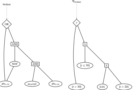
Example 4. Consider our initial example in Eq. 1. Executing the first two steps of Symbo yield the compiled logic formula that is shown on the left in Figure 1. Steps number three and four of Symbo produce the arithmetic circuit on the right in Figure 1. The probability for the theorybroken, which
NOT
abst>30 no cool abst>20
AND
AND OR
broken
[t≤30]
[t>30] 0.01 [t>20]
×
×
+ Ψbroken
Figure 1: Shown on the left is a graphical representation of the compiled logic formula given in Eq. 1 (in the SDD target language), where the atomic formulas have been abstracted away. On the right we see the corresponding arithmetic circuit where the literals have been replaced by corresponding labels according to the labeling function in 9 and where the logic and/or operation have been replaced by ×/+ respectively. Note, the labels in the arithmetic circuit do not explicitly state the set of continuous variables involved.
coincides with the weighted model integral, is obtained by evaluating the arithmetic circuit (step five), multiplying this expression by the probability density function fort(step six) and carrying out the integral (step 7).
p(broken)
=R
(0.01[t>20][t≤30]+[t>30])Nt(20,5)dt =0.01R20<t≤30Nt(20,5)dt+
R
t>30Nt(20,5)dt
=1−0.01R−
5√8 2 +
20
√
8
−∞ e
−x2
dx−0.99R− 5√8
2 + 30
√
8
−∞ e
−x2
dx
In Example 4, the weight function on the continuous vari-ables depended only on a single variable. It is, however, easy to see that our formalism does also allow for multivariate dis-tributions that are then used with more intricated integration bounds, such as in Example 3.
5.2
Sampo
In the general case, symbolic inference methods are not able to produce numerical results to a given problem. This is because the resulting integrals are not tractable utilizing sym-bolic integration. For such cases Monte Carlo (MC) methods are used to compute intractable integrals by approximating the integration by a summation.
2For a detailed discussion of allowed symbolic manipulations
Theorem 3. (MC approximation of WMI) Let φ be an SMT(RA) theory,wa factorizable weight function over the Boolean variables Band continuous variables X. Further-more, letAMC(φ,w|X∪B) evaluate to (Ψ,V(Ψ)). Then the Monte Carlo approximation of WMI(φ,w|X,B) is given by:
W MIMC(φ,w|X,B)B N1 PN
i=1Ψ(xi) (11)
where thexi’s areNindependent and identically distributed
random variables drawn from the densityw. Proof.
W MI(φ,w|X,B)=Rx∈XΨ(x)wx(x)dx P1
=Ewx(x)[Ψ(x)] P2
≈ N1 PN
i=1Ψ(xi) P3
The expression in P2 denotes the expectation ofΨ(x) with respect tow(x). The approximation in P3 is the mean value ofΨ obtained through MC assignments to the continuous
random variables present inΨ.
The MC approximation of the weighted model integral of an SMT formula necessitates that we evaluate a compiled SMT problem atNdifferent points, i.e. we need to evaluate a compiled theoryN times with different weights. This is exactly where the strength of knowledge compilation lies: expensively compile once and cheaply evaluate often.
Numerical computation libraries such as TensorFlow rely heavily on the concept of computation graphs. Realizing that we can translate a d-DNNF formula to a computational graph and express the labels of literals in an SMT formula as tensors, allows us to compute theNevaluations necessary for the MC approximation of the weighted model integral not only cheaply but also in parallel.
Algorithm 2. Sampo computes the weighted model integral of an SMT(RA) formulaφfor a factorizable weight functionwby executing the following steps:
1. Abstract all atomic formulas inφaccording to Defi-nition 8 and obtainφa.
2. Compileφainto a d-DNNF representationφcompiled.
3. Transformφcompiledinto an arithmetic circuitACφ, i.e.
replacing logical and/or operations with elementwise tensor multiplications/additions.
4. Label the literals inACφ according to the labeling function given in Definition 9 with corresponding tensors.
5. Symbolically evaluateACφand obtain (Ψ,V(Ψ))
rep-resented by a computation graphCG.
6. Run theCGrepresenting (Ψ,V(Ψ))Ntimes, where
Nis the number of samples approximating the proba-bility densities.
7. Take the mean of the values of the N runs of the CG.
We implemented Algorithm 2 using again the SDD pack-age for the KC step and using TensorFlow as the underlying symbolico-numerical computation library. Random variables are sampled using the Edward library.
Example 5. Let us illustrate Sampo on our running example in Eq. 1. Assume therefore that we already have at hand
ACEvaluatedφ . We then need to sampleNvalues for the random variablet. Lets suppose we sample 5 values.
tMC∈ {12.8,35.1,17.6,22.2,21.4} (13)
and plug these samples intoΨ. We map the Boolean random variableno coolto a 1Dtensor whose entries are 0.01. Con-sulting the arithmetic circuit in Figure 1, we easily see that we obtain for the MC estimate:
ΨMC=
0.01 0.01 0.01 0.01 0.01
◦
[12.8>20] [35.1>20] [17.6>20] [22.2>20] [21.4>20]
◦
[12.8≤30] [35.1≤30] [17.6≤30] [22.2≤30] [21.4≤30]
+
[12.8>30] [35.1>30] [17.6>30] [22.2>30] [21.4>30]
=
0.01 0.01 0.01 0.01 0.01
◦ 0 1 0 1 1 ◦ 1 0 1 1 1 + 0 1 0 0 0 = 0 1 0 0.01 0.01
(14)
where◦denotes the elementwise multiplication of tensors. With the Monte Carlo estimate ofΨwe obtain the MC esti-mate for the weighted model integral by simply averaging:
W MIMC=
1 5
P5
i=1ΨMC,i=1.02/5=0.204
Compiling an SMT formula and transforming the resulting arithmetic circuit into a computation graph has the advantage that sampling becomes embarrassingly parallelizable. To the best of our knowledge, Sampo is the first probabilistic infer-ence algorithm for the hybrid domain that is able to harness parallelization on a GPU.
5.3
Discussion on Complexity
The complexity of Symbo and Sampo is mainly determined by the complexity of their subcomponents. The knowledge compilation step is #P-complete. The evaluation of the result-ing arithmetic circuit is done in polytime. Symbo, however, suffers from the problem that the search for simplifications in symbolic expressions is a hard problem. One such simpli-fication is the symbolic integration step itself. For example, integrating convex polytopes is #P-complete. These complex-ity concerns do not hold for Sampo, as we are dealing with mere additions and multiplications on the GPU.
In the next section the computational complexity of sym-bolic simplifications becomes experimentally apparent in the ClickGraph benchmark for Symbo (cf. Table 1). We are cur-rently already investigating how to practically circumvent the computational hardness in such cases. For example, by sub-querying or by static program analysis and detecting where to intermediately integrate variables.
6
Experimental Evaluation
weight functions), we compare Symbo and Sampo with state-of-the-art inference algorithms in probabilistic programming. To this end, we extended the syntax of the probabilistic programming system ProbLog2 (Dries et al. 2015), so that it allows for the use of abstractions of atomic formulas and for the declaring how continuous random variables are dis-tributed. ProbLog2 implements inference for the probabilistic programming language aProbLog (Kimmig, Van den Broeck, and De Raedt 2011), where inference is done through alge-briac model conting.
We are interested in two main questions during the ex-perimental evaluation of Symbo and Sampo.Q1:How does Symbo, a logico-symbolic solver, compare to a pure, state-of-the-art, symbolic solver for the hybrid domain?Q2:How does Sampo compare to related state-of-the-art probabilistic inference algorithms?Q3:In the interest of completeness we also adopted Symbo to solve traditional weighted model integration problems, where the weight function is expressed as a polynomial function.
We answerQ1by comparing Symbo, which uses the PSI-Solver and combines it with KC, to pure symbolic inference with the PSI-Solver.
ForQ2, we compare Sampo to the inference algorithms of Distributional Clauses (DC) (Nitti, De Laet, and De Raedt 2016)3, BLOG (Milch et al. 2007)4 and to Hybrid Proba-bilistic Model Counting (IHPMC) (Michels, Hommersom, and Lucas 2016)5. These are state-of-the-art probabilistic programming systems that all support first order logic as well as hybrid representations.
InQ3we compare Symbo to the existing WMI solver of (Morettin, Passerini, and Sebastiani 2017), which uses predi-cate abstraction, SMT solving and numerical integration, and to the solver of (Kolb et al. 2018), which uses XADDs (San-ner and Abbasnejad 2012) and hence symbolic integration.
Experiments were performed on a laptop Intel(R) i7 CPU 2.60GHz with 16 Gb memory. Sampo took additionally ad-vantage of an NVIDIA Quadro M1000M.
Q1 (Symbo): We compared Symbo and the PSI-Solver on the set of benchmark experiments given in (Gehr, Misailovic, and Vechev 2016, section F of Appendix)6.
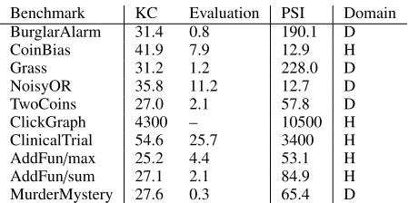
In Table 1, we observe that Symbo outperforms the PSI-Solver for 9/10 benchmarks, for 7/10 even when including the time spent on the knowledge compilation step. Only for the ClickGraph benchmark PSI performs better than Symbo, which timed-out after 15s during circuit evaluation. This is because PSI integrates out variables after loop iterations. This is not yet supported in the ProbLog implementation and Symbo ends up with a large symbolic expression that is hard to integrate over. This could be solved, for example, by using sub-queries, as can be done in ProbLog2.
We note that the symbolic inference engine underlying the PSI-Solver has until now only been used for imperative programing. The implementation of Symbo shows that the
3https://bitbucket.org/problog/dc problog
4https://bayesianlogic.github.io
5https://github.com/SteffenMichels/IHPMC
6cf.: Fun (Minka et al. 2014) and R2 (Nori et al. 2014)
Benchmark KC Evaluation PSI Domain
BurglarAlarm 31.4 0.8 190.1 D
CoinBias 41.9 7.9 12.9 H
Grass 31.2 1.2 228.0 D
NoisyOR 35.8 11.2 12.7 D
TwoCoins 27.0 2.1 57.8 D
ClickGraph 4300 – 10500 H
ClinicalTrial 54.6 25.7 3400 H
AddFun/max 25.2 4.4 53.1 H
AddFun/sum 27.1 2.1 84.9 H
MurderMystery 27.6 0.3 65.4 D
Table 1: Knowledge compilation and arithmetic circuit eval-uation times for Symbo, and problem solving time for PSI. Times are given in ms. Run times were averaged over 50 runs. The domain column indicates whether the problem is Discrete orHybrid.
powerful symbolic inference engine can also be adopted for logic programming when making use of KC.
To conclude, it is generally beneficial to perform logical inference on top of symbolic inference in the hybrid domain.
Q2 (Sampo): In order to evaluate Sampo, we chose bench-marks from (Nitti, De Laet, and De Raedt 2016) and (Michels, Hommersom, and Lucas 2016), which were stated to be hard-est in terms of query complexity. We show our results in Figures 2 and 3. In Figure 2, we compare Sampo to DC and BLOG. A comparison with IHPMC for this first problem is not possible as IHPMC does not allow for expressing hierar-chical models. DC an BLOG are, just like Sampo, sampling based methods, which use both importance sampling and likelihood weighting7. This is why we plot the evaluation time and the standard deviation in function of the number of samples. IHPMC is not a sampling based method but it-eratively splits up the space into mutually exclusive pieces and calculates bounds for each piece, which translates to it-eratively tighter and tighter error bounds. For this reason we investigate in the plots in Figure 3 the standard deviation of the four methods scrutinized in function of the run time.
All four plots clearly indicate that once Sampo has trans-formed a probabilistic program into an arithmetic circuit, the run time is not only lower but also that Sampo is more accu-rate than the competing algorithms. This is especially true for two distinct cases. Firstly, when there are binary random vari-ables present. Contrary to DC and BLOG, Sampo does not sample these random variables but includes their probability as weight in the circuit evaluation. This can be seen Figure 2a and 3a. The reason why the STD is not zero for Sampo in 2a is due to floating point rounding errors. The second case where Sampo clearly outperforms the other methods is when we condition on low probability events, cf. Figure 3b. Here we condition on an event that has probability 0.0001 to occur. The logic structure of the problem implies that the query given the observation must be satisfied. In Figure 3b we see that Sampo is the only algorithm that picks up this structure. As the inference reduces to inference on exclusviely Boolean
0.0 0.5 1.0 1.5
run time [s]
Sampo DC BLOG
102 103 104 105 106 107
number of samples
108
106
104
102
STD
(a)
0 1 2
run time [s]
Sampo DC BLOG
102 103 104 105 106 107
number of samples
103
102
101
STD
(b)
Figure 2: The example used isdrawing balls (denoted by bi and having different size, color and material) with
re-placement from an urn(Nitti, De Laet, and De Raedt 2016). The queries used are (a) p(b1=b2∧col(b1)=black) and (b)
p(b1=1|0.39<size(b1)<0.41). The upper panel shows the run
time (circuit evaluation for Sampo). Evaluation runs are av-eraged over 50 runs and the knowledge compilation step is averaged over 50 compilations. Time-out was set at 2.5s. The linear behavior of Sampo towards higher sample numbers is due to the GPU starting to run out of memory. Sampo spent 1.62s for (a) and 0.11s for (b) on the knowledge compilation step, averaged over 50 runs.
random variables, Sampo immediately finds the correct so-lution without drawing any samples for continuous random variables, in contrast to the other algorithms.
We also observe that there is practically no time penalty for the number of samples for Sampo, contrary to DC and BLOG. This behavior manifests itself most prominently in the upper panel of Figure 2a and in Figure 3a. For the latter, we see that higher sample numbers, which correspond to lower STDs, take up just as much time as lower sample numbers. This produces the quasi-vertical line Figure 3a. This behavior is due to delegating theNevaluations of the arithmetic circuits, which correspond toN times sampling the continuous random variables, to the GPU and executing the evaluation in parallel. Only in Figure 2a we observe a linear dependency of the run time in function of the number of samples towards high sample numbers. This is caused by the GPU running out of memory.
Q3 (WMI): By allowing Symbo to handle also bounded polynomial weights, instead of probability density distribu-tions, we can compare Symbo to the existing exact WMI solvers of WMI-PA (Morettin, Passerini, and Sebastiani 2017) and WMI-XADD (Kolb et al. 2018). This extension of Symbo is necessary as these solvers are limited to polynomial weights and cannot handle proper probability densities.
We made the experimental comparison of the three meth-ods on a set of synthetic problems given in (Morettin, Passerini, and Sebastiani 2017)8. The benchmarks consist of
WMI problems that have from five to seven Boolean variables
8https://github.com/unitn-sml/wmi-pa
0.0 0.5 1.0 1.5 2.0
Inference time [s]
103
102
101
100
MSE
Sampo DC BLOG IHPMC
(a) query:p(f99)
0.0 0.5 1.0 1.5
Inference time [s] 0.0
0.5 1.0
MSE
Sampo DC BLOG IHPMC
(b) query:p(f99|f0)
Figure 3: We show the dependencies of the mean squared error on time for two queries of the theory: fi ↔ di∨c>
li∨ fi−1, cf. (Michels, Hommersom, and Lucas 2016). fiand
diare Bools. The probability ofdibeing true is 0.0001.cand
li are normally distributed variables with mean 20 and 30
respectively and standard deviation 5. Note the two different scales for the plots on the y-axis. The mean squared errors are averaged over 50 runs. The average KC time (over 50 iterations) is 4.34s for (a) and 2.66s for (b). In the left plot the mean squared error was calculated with respect to the mean of 50 runs using Sampo with 105samples. In the right plot, we stopped when all the runs for a given number of samples for an algorithm reached the correct solution (which is 1.0) or the algorithm timed-out after 2s.
and where the weight functions are multivariate polynomials of dimensions two to three.
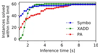
We compared the three methods on the benchmarks with two dimensional polynomial weights. We observe in Figure 4 that Symbo solves the majority of the problems with bivariate polynomials faster than the other two methods. We omit the comparison plot for the benchmarks with three dimensional polynomials, as here the other methods, which are specialized algorithms for polynomial weight functions, beat Symbo at large. Symbo spends most of the time on the final integration step (cf. point 7 in Algorithm 1). In fact, Symbo spent at most 0.32s on the KC step, at most 0.34s on the circuit evaluation and any remaining time on the symbolic integration - for any of the presented benchmarks. Using a dedicated integrator for bounded polynomials instead of the generic PSI inte-grator could mitigate this problem. Integrating out variables during the evaluation of the arithmetic circuit could also be beneficial, as this leads to smaller symbolic expressions.
2 4 6 8 10 Inference time [s]
0 20 40 60
Instances solved within time limit
Symbo XADD PA
7
Related Work
In the initial work on weighted model integration (Belle, Passerini, and Van den Broeck 2015) the authors perform weighted model integration on piecewise polynomials by it-eratively generating models by adding the negation of the model from the previous iteration to the formula. In subse-quent work by (Morettin, Passerini, and Sebastiani 2017) the number of generated models is substantially reduced by deploying SMT-based predicate abstraction (Graf and Sa¨ıdi 1997). In this line of work (Belle et al. 2016) also investigated component caching while performing a DPLL search when calculating a weighted model integral. Their approach is in-deed related to knowledge compilation. However, it is not applicable in cases when algebraic constraints exist between variables and couple these. The methods proposed on WMI are strictly limited to piecewise polynomials. We, completely lift this restrictions and are able to perform WMI via knowl-edge compilation on SMT(RA) and SMT(N RA) formulas using probability density functions instead of piecewise poly-nomials on SMT(LRA).
As seen in section 6, WMI has also been studied in the context of XADDs (Kolb et al. 2018) and the approach is closely related to Symbo. Here again, the weight functions considered are only of polynomial form. Another drawback of this approach is that, unlike for the SDDs and d-DNNFs used in our approach, there are not yet any efficient com-pilers available for converting WMI to XADDs. For SDDs and d-DNNFs, one can employ standard state-of-the-art KC technology. SDDs are more succinct than BDDs, of which XADDs are an extension. This entails, in turn, that SDDs are more succinct than XADDs. Standard knowledge compila-tion techniques are not readily available for XADDs as Kolb et al.’s compilation algorithm interleaves symbolic and logic inference.
Somewhat related to WMI with piecewise polynomials is the work of (Gutmann, Jaeger, and De Raedt 2011), who restricted distributions to Gaussians, which are chopped up into easily integrable and axis-aligned pieces.
Contrary to these works, we generalize WMI by providing a much larger class of weight functions and constraints.
With respect to inference for probabilistic programming in the hybrid domain, two classes of algorithms exist: approxi-mate and exact. Firstly, for what concerns one of the few exact inference systems, there is the already mentioned work for imperative probabilistic programming (Gehr, Misailovic, and Vechev 2016), which has contributed the PSI-Solver that we use in Symbo. The PSI-Solver beats other recent approaches in exact probabilistic inference (Narayanan et al. 2016). We show that knowledge compilation speeds up pure symbolic inference and that Symbo outperforms the PSI-Solver.
Another approach, related to exact inference in proba-bilistic logic programming, is that of (Islam, Ramakrishnan, and Ramakrishnan 2012). Similarly to Symbo, they symboli-cally evaluate a theory in order to obtain an expression for a probability density. However, their approach is restricted to Gaussians (although gamma distributions are in theory also implementable), and more importantly it is built on top of Prism (Sato 1995), which assumes that proofs are mutually exclusive, and which avoids the disjoint sum problem. As a
consequence they do not support WMI in its full generality. Supporting WMI requires the KC step, which they do not address.
Secondly, for what concerns approximate inference, we have the sampling approaches in Distributional Clauses by (Gutmann et al. 2011; Nitti, De Laet, and De Raedt 2016) and BLOG by (Milch et al. 2007), which we have already discussed in section 6 and which both deploy importance sampling in order to sample from probability distributions and densities alike, combined with likelihood weighting.
Approximate inference is also performed in (Michels, Hommersom, and Lucas 2016). In their work, a hybrid prob-abilistic problem is represented by so calledhybrid proba-bility trees(discussed in Section 6). Our experiments show that Sampo outperforms DC, BLOG and IHPMC. Moreover, Sampo has the advantage that when conditioning on rare events in the discrete domain, we still obtain reliable esti-mates of the weighted model integral. Using pure sampling based methods such as in Distributional Clauses and BLOG leads to poor results. This is known to be problematic when using importance sampling based methods.
Note that when conditioning on rare events in continu-ous domains, Sampo performs as poorly as other sampling techniques as it performs essentially rejection sampling with almost all samples being rejected.
8
Conclusion and Future Work
We have shown how knowledge compilation can be applied to the task of weighting model integration by leveraging algebraic model counting and thereby presenting a unified formalism for weighted model integration and knowledge compilation. We have also introduced an exact and an ap-proximate solver based on this idea and demonstrated their effectiveness. Sampo is to the best of our knowledge the first sampling based algorithm deployable in the WMI setting.
In future work, we would like to investigate in more detail the relationship between Kolb et al.’s work and the work presented here, theoretically as well as experimentally. More-over, we would like to integrate Symbo and Sampo into a full-fledged probabilistic programming language and investigate thoroughly how it compares to existing languages, especially DC, BLOG, Anglican, Church.
9
Acknowledgments
This work has been supported by the Research Founda-tion - Flanders (FWO) project G0D7215N, the European Research Council Advanced Grant project SYNTH9
(ERC-AdG-694980), and the H2020 CHIST-ERA and FWO project ReGround10(G0D7215N). The authors would like to thank
Sebastijan Dumanˇci´c, Angelika Kimmig, Ondˇrej Kuˇzelka and Robin Manhaeve for reading and commenting on first drafts of this paper, and Samuel Kolb for inspiring discus-sions on the topic of WMI.
References
Abadi, M.; Agarwal, A.; Barham, P.; Brevdo, E.; Chen, Z.; Citro, C.; Corrado, G. S.; Davis, A.; Dean, J.; Devin, M.; Ghemawat, S.; Goodfellow, I.; Harp, A.; Irving, G.; Isard, M.; Jia, Y.; Jozefowicz, R.; Kaiser, L.; Kudlur, M.; Levenberg, J.; Man´e, D.; Monga, R.; Moore, S.; Murray, D.; Olah, C.; Schuster, M.; Shlens, J.; Steiner, B.; Sutskever, I.; Talwar, K.; Tucker, P.; Vanhoucke, V.; Vasudevan, V.; Vi´egas, F.; Vinyals, O.; Warden, P.; Wattenberg, M.; Wicke, M.; Yu, Y.; and Zheng, X. 2015. TensorFlow: Large-Scale Machine Learning on Heterogeneous Systems. Software available from tensorflow.org.
Belle, V.; Van den Broeck, G.; Passerini, A.; et al. 2016. Component Caching in Hybrid Domains with Piecewise Poly-nomial Densities. InAAAI, 3369–3375.
Belle, V.; Passerini, A.; and Van den Broeck, G. 2015. Prob-abilistic Inference in Hybrid Domains by Weighted Model Integration. InProceedings of 24th International Joint Con-ference on Artificial Intelligence (IJCAI), 2770–2776. Chavira, M., and Darwiche, A. 2008. On Probabilistic In-ference by Weighted Model Counting.Artificial Intelligence
172(6):772 – 799.
Choi, A.; Kisa, D.; and Darwiche, A. 2013. Compiling Probabilistic Graphical Models Using Sentential Decision Diagrams. Berlin, Heidelberg: Springer Berlin Heidelberg. 121–132.
Darwiche, A., and Marquis, P. 2002. A Knowledge Compila-tion Map.J. Artif. Int. Res.17(1):229–264.
Dries, A.; Kimmig, A.; Meert, W.; Renkens, J.; Van den Broeck, G.; Vlasselaer, J.; and De Raedt, L. 2015.ProbLog2: Probabilistic Logic Programming. Cham: Springer Interna-tional Publishing. 312–315.
Fierens, D.; Van den Broeck, G.; Renkens, J.; Shterionov, D.; Gutmann, B.; Thon, I.; Janssens, G.; and De Raedt, L. 2015. Inference and Learning in Probabilistic Logic Programs Us-ing Weighted Boolean Formulas. Theory and Practice of Logic Programming15(3):358–401.
Fubini, G. 1907. Sugli Integrali Multipli.Rom. Acc. L. Rend. (5)16(1):608–614.
Gehr, T.; Misailovic, S.; and Vechev, M. 2016. PSI: Exact Symbolic Inference for Probabilistic Programs. In Interna-tional Conference on Computer Aided Verification, 62–83. Springer.
Graf, S., and Sa¨ıdi, H. 1997. Construction of Abstract State Graphs with PVS. InInternational Conference on Computer Aided Verification, 72–83. Springer.
Gutmann, B.; Thon, I.; Kimmig, A.; Bruynooghe, M.; and De Raedt, L. 2011. The Magic of Logical Inference in Probabilistic Programming. Theory and Practice of Logic Programming11(4-5):663–680.
Gutmann, B.; Jaeger, M.; and De Raedt, L. 2011. Extending ProbLog with Continuous Distributions. Berlin, Heidelberg: Springer Berlin Heidelberg. 76–91.
Islam, M. A.; Ramakrishnan, C.; and Ramakrishnan, I. 2012. Inference in Probabilistic Logic Programs with Continuous
Random Variables. Theory and Practice of Logic Program-ming12(4-5):505–523.
Kimmig, A.; Van den Broeck, G.; and De Raedt, L. 2011. An Algebraic Prolog for Reasoning about Possible Worlds. InAAAI.
Kimmig, A.; Van den Broeck, G.; and De Raedt, L. 2017. Algebraic Model Counting.Journal of Applied Logic22:46– 62.
Knuth, D. E. 1992. Two Notes on Notation. Am. Math. Monthly99(5):403–422.
Kolb, S.; Mladenov, M.; Sanner, S.; Belle, V.; and Kersting, K. 2018. Efficient Symbolic Integration for Probabilistic Inference. InIJCAI, 5031–5037.
Michels, S.; Hommersom, A.; and Lucas, P. J. F. 2016. Ap-proximate Probabilistic Inference with Bounded Error for Hybrid Probabilistic Logic Programming. InIJCAI 2016. Milch, B.; Marthi, B.; Russell, S.; Sontag, D.; Ong, D. L.; and Kolobov, A. 2007. BLOG: Probabilistic Models with Un-known Objects. In Getoor, L., and Taskar, B., eds.,Statistical Relational Learning. MIT Press.
Minka, T.; Winn, J.; Guiver, J.; Webster, S.; Za-ykov, Y.; Yangel, B.; Spengler, A.; and Bronskill, J. 2014. Infer.NET 2.6. Microsoft Research Cambridge. http://research.microsoft.com/infernet.
Morettin, P.; Passerini, A.; and Sebastiani, R. 2017. Effi -cient Weighted Model Integration via SMT-Based Predicate Abstraction. def1(x1):x2.
Narayanan, P.; Carette, J.; Romano, W.; Shan, C.; and Zinkov, R. 2016. Probabilistic Inference by Program Transformation in Hakaru (System Description). InInternational Symposium on Functional and Logic Programming - 13th International Symposium, FLOPS 2016, Kochi, Japan, March 4-6, 2016, Proceedings, 62–79. Springer.
Nitti, D.; De Laet, T.; and De Raedt, L. 2016. Probabilistic Logic Programming for Hybrid Relational Domains. Ma-chine Learning103(3):407–449.
Nori, A. V.; Hur, C.-K.; Rajamani, S. K.; and Samuel, S. 2014. R2: An Efficient MCMC Sampler for Probabilistic Programs. InAAAI, 2476–2482.
Sanner, S., and Abbasnejad, E. 2012. Symbolic Variable Elimination for Discrete and Continuous Graphical Models. InAAAI.
Sato, T. 1995. A Statistical Learning Method for Logic Programs with Distribution Semantics. InIn proceedings of the 12TH international conference on logic programming (ICLP’95. Citeseer.