The Thirty-Third AAAI Conference on Artificial Intelligence (AAAI-19)
MFPCA: Multiscale Functional Principal Component Analysis
Zhenhua Lin
University of California, Davis One Shields Avenue, Davis, CA 95616Hongtu Zhu
University of North Carolina at Chapel Hill Chapel Hill, NC 27599
Abstract
We consider the problem of performing dimension reduc-tion on heteroscedastic funcreduc-tional data where the variance is in different scales over entire domain. The aim of this paper is to propose a novel multiscale functional principal component analysis (MFPCA) approach to address such het-eroscedastic issue. The key ideas of MFPCA are to partition the whole domain into several subdomains according to the scale of variance, and then to conduct the usual functional principal component analysis (FPCA) on each individual sub-domain. Both theoretically and numerically, we show that MFPCA can capture features on areas of low variance with-out estimating high-order principal components, leading to overall improvement of performance on dimension reduction for heteroscedastic functional data. In contrast, traditional FPCA prioritizes optimizing performance on the subdomain of larger data variance and requires a practically prohibitive number of components to characterize data in the region bear-ing relatively small variance.
1
Introduction
Functional principal component analysis (FPCA) is a key tool for performing dimension reduction on functional data that features infinite dimensionality and emerges in many machine learning applications (Ghebreab, Smeulders, and Adriaans 2008; Ramsay and Silverman 2005; Ferraty and Vieu 2006; Hsing and Eubank 2015). In classic FPCA re-ferred to assingle-scaleFPCA in this paper, a single eigen-analysis is conducted for observed functions on theentire
domain. Specifically, FPCA is built on eigen-analysis of the covariance function of functional data, analogous to the co-variance matrix, from which we derive functional princi-pal components. For the purpose of dimension reduction, only the principal components corresponding to the first few largest eigenvalues are retained. Related works include early development of FPCA (Rao 1958; Dauxois, Pousse, and Ro-main 1982; Besse and Ramsay 1986), and more recent ad-vances such regularization techniques (Rice and Silverman 1991; Silverman 1996), estimation and theory (Yao, M¨uller, and Wang 2005; Hall, M¨uller, and Wang 2006; Li and Hs-ing 2010; Zhang and Wang 2016) for functional data that are sparsely observed, and interpretability (Chen and Lei 2015;
Copyright c2019, Association for the Advancement of Artificial Intelligence (www.aaai.org). All rights reserved.
Lin, Wang, and Cao 2016), to name a few. All of these works adopt the single-scale paradigm, which is briefly described in the next section.
Such one-size-fits-all scheme, as we show in Section 2, inevitably comes with a side effect that the leading principal components prioritize producing good approximation qual-ity for functions on the subdomain that holds large data vari-ance. However, for heteroscedastic functional data, where the variance of the data has substantially different scales over the domain, single-scale FPCA approach often needs a large number of principal components in order to charac-terize the behavior of the data on the subdomain with rel-atively small variance. However, it is notoriously difficult to accurately estimate high-order principal components. For example, for a fixed sample size, the estimation error for thekth principal components is approximately of the order k2(Mas and Ruymgaart 2015). This quadratic decay in es-timation quality prohibits one from obtaining reliable esti-mates of principal components for a moderate sample size except for the first few leading ones. Consequently, for het-eroscedastic functional data, single-scale FPCA may not be able to discover useful features in the area of low variance.
To address the issue of FPCA for heteroscedastic func-tional data, we consider a question, which states
“Could we modify standard FPCA to efficiently deal with heteroscedastic functional data?”
Our solution to the above question is the development of a novelmultiscale FPCA framework. The key ideas of MF-PCA are to partition the whole domain into several subdo-mains in the way that the variance of the data within a sub-domain is approximately on the same scale, and then to con-duct FPCA on each subdomain separately. Compared with the existing methods in the literature, three major method-ological contributions in this paper are as follows:
• Our MFPCA approach is simple and yet powerful. Specif-ically, compared to single-scale FPCA, the multiscale ap-proach alleviates the issue of estimating high-order princi-pal components and leads to overall improvement of data representation, since fewer components are required for sufficient approximation of the data within each subdo-main.
brain microstructure in relation to multiple sclerosis us-ing diffusion tensor imagus-ing techniques; see Section 4 for details.
• Theoretically, we show that MFPCA has larger capac-ity of representation for functional data and yields higher estimation quality for principal components than single-scale FPCA. The theoretical analysis is complemented by numerical simulation in Section 4.
2
Classic Functional Principal Component
Analysis
Without loss of generality, let X be a random process de-fined on an intervalIsuch thatEkXk2
L2 <∞andEX = 0. FPCA is built on the concept of Karhunen-Lo`eve expansion ofX. Specifically,X(t)admits the following representation
X(t) = ∞ X
k=1
ξkφk(t), (1)
whereξk are centered uncorrelated random variables,φk(·) are normalized eigenfunctions of the covariance function
C(s, t) = Cov{X(s), X(t)}, andVar(ξk), often denoted by λk, is the eigenvalue ofCcorresponding toφk, i.e.,
Z
I
C(·, t)φk(t)dt=λkφk(·). (2)
It is also conventionally assumed thatλ1 > λ2 >· · · >0.
The eigenfunctionsφ1(·), φ2(·), . . ., referred to as principal
components in the context of FPCA, form an orthonormal basis ofL2(I).
The above FPCA is a single-scale approach in the sense that both (1) and (2) are defined on the entire intervalI. It has the following global optimality of Karhunen-Lo`eve ex-pansion for approximation of X using the first few eigen-functions. For any fixed K > 0, let B = {B1, . . . , BK}
be a collection ofK orthonormal real-valued functions in
L2(I), and define P
Bthe projection operator of the space
spanned byB1, . . . , BK, i.e., PBX = P
K
k=1hBk, XiBk,
wherehBk, Xi=R
IBk(t)X(t)dt. In principle,PBXis the approximation ofX using the basis functionsB1, . . . , BK. The approximation error is often measured by E(B) =
E kX−PBXk2L2
. It can then be shown that E(Φ) ≤ E(B)forΦ={φ1, . . . , φK}and anyBofKorthonormal
functions inL2(I).
Although such optimality of single-scale FPCA is attrac-tive for approximating functional data, it has an undesired side-effect for functional data with different scales of vari-ability on the interval I. To elaborate, we divide I into J equal subintervalsI1, . . . , IJthat form a partition ofI, in the sense thatSJ
j=1Ij=IandIj∩Ik =∅for1≤j6=k≤J.
DenoteX(j)(t)as the restriction ofX(t)to the subinterval
Ij, i.e.,X(j)(t) =X(t)ift∈IjandX(j)(t) = 0ift6∈Ij.
Then, we have
E(B) =E kX−PBXk2L2
=
J
X
j=1
EkX(j)−(PBX)(j)k2L2
=E kXk2
L2
×
J
X
j=1
E kX(j)−(P
BX)(j)k2L2
E kX(j)k2
L2
E kX(j)k2
L2
E kXk2
L2
,
where(PBX)(j)denotes the restriction ofPBX toIj. Let
wj = E kX(j)k2
L2
/E kXk2
L2
for all j ≤ J, which are constants that are independent of B. We interpret the weightswj as the variance density ofX onIj. Then, find-ingBto optimizeE(B), which the single-scale FPCA does, prioritizes minimizing the approximation error for the pieces with larger weights, i.e., with relatively larger variance den-sity. Therefore, in order to capture features of pieces that have small weights, one needs a large number of principal components. As the principal componentsφk are unknown, one needs to estimate them from a finite sample. However, it is difficult to estimate the high-order principal components, in light of the fact that any estimate for φk based onn in-dependently and identically distributed (i.i.d.) samples ofX cannot have an estimation error less than ck2/nfor some constant c > 0 (Mas and Ruymgaart 2015). Thus, if one applies single-scale FPCA toX(t)that exhibits multiscale variability overI, then the features in the area with low vari-ance density might be concealed by those in the region of high variance density.
3
Multiscale Karhunen-Lo`eve Expansion
To overcome the aforementioned shortcoming of single-scale FPCA, for heteroscedastic functional data, we adopt the following simple divide-and-conquer strategy to con-duct FPCA: divide the interval I into several subintervals according to the scale of variance on I, and then per-form FPCA on each subinterval. To be more precise, let I1, . . . , IJ and X(1), . . . , X(J) be defined as in Section 2. Applying single-scale FPCA to each X(j) on Ij, we can obtain the Karhunen-Lo`eve approximation X(j)(t) ≈PKj
k=1ξ (j)
k φ
(j)
k (t), whereφ
(j)
k is thekth leading eigenfunc-tion of the multiscale covariance funceigenfunc-tionC(j)that is defined
byC(j)(s, t) = Cov{X(j)(s)X(j)(t)}on the squareI
j×Ij. The approximation forX is then obtained by
X(t)≈
J
X
j=1
Kj X
k=1
ξ(kj)φ(kj)(t). (3)
Although there arePJ
j=1Kj terms in (3), for eacht ∈Ij,
onlyKj of them are nonzero asφ
(j)
onIj, then a relatively larger number of principal compo-nents can be used to obtain a good approximation, while for relatively smooth pieces,X(k), a small number might
be sufficient. In contrast, single-scale FPCA uses the same number of principal components for eacht ∈ I and hence does not enjoy such extra adaptivity. Note that (3) automati-cally takes into account the fact that the sub-domains where the data have small variance contribute less than others to approximating the processX(t), by observing that the prin-cipal component scores ξk(j) have different scales of vari-ance on different sub-domains. For those sub-domains with small variance, the scale of the corresponding principal com-ponent scores is also small. Nevertheless, the features of a small scale could be influential in supervised learning tasks, as demonstrated in Section 4.
As stated previously, single-scale FPCA has the global optimality property, which can be equivalently stated as
EkPΦXk2L2 ≥ EkPBXk2L2, whereΦ andB are defined in Section 2. The quantityEkPΦXk2L2 is often interpreted as the amount of variance explained by the principal compo-nents inΦ. The optimality property essentially asserts that the firstKeigenfunctions explain the variance ofX more than any other K orthonormal functions for any K ≥ 1. However, by exploring local adaptivity, our MFPCA enjoys larger capacity of representation of functional data, i.e., it can explain larger variance than single-scale FPCA when the same number of principal components is used to approx-imateX(t)for eacht∈I. The following proposition illus-trates this point forK= 1.
Proposition 1. LetI1, . . . , IJform a disjoint partition ofI.
Suppose thatXis a random process satisfyingEkXk2
L2 <
∞ and (without loss of generality) EX = 0. Let Sj be
the collection of function f such that kfk2
L2 = 1 and
support(f)⊂Ij. Then
EkPφ1Xk2L2 =EhX, φ1i2≤ sup
ψ(j)∈Sj J
X
j=1
EhX, ψ(j)i2.
The equality is possible only ifEhX, φ(1j)i=EhX, φ(1k)ifor
all1 ≤j, k ≤ J, whereφ(1j)denotes the restriction of the
single-scale eigenfunctionφ1ontoIj.
Proof. It is easy to see that the conclusion holds forJ >
2 if it is true for J = 2. Suppose kφ(1)1 kL2 > 0 and
kφ(2)1 kL2 > 0; otherwise, the conclusion is trivial. Set
˜
φ1=φ (1) 1 /kφ
(1)
1 kL2andφ˜2=φ (2) 1 /kφ
(2)
1 kL2. Then
EhX, φ1i2=EhX, φ
(1)
1 +φ
(2)
1 i
2
=EhX, φ(1)1 i2+EhX, φ(2)
1 i
2+ 2E(hX, φ(1)
1 ihX, φ
(2) 1 i)
=kφ(1)1 k2
L2EhX,φ˜1i2+kφ (2)
1 k
2
L2EhX,φ˜2i2
+ 2kφ(1)1 kL2kφ
(2)
1 kL2E(hX,φ˜1ihX,φ˜2i)
≤ kφ(1)1 k2L2EhX,φ˜1i2+kφ (2)
1 k
2
L2EhX,φ˜2i2
+kφ(1)1 k2
L2EhX,φ˜2i2+kφ (2)
1 k
2
L2EhX,φ˜1i2
=EhX,φ˜1i2+EhX,φ˜2i2,
where the last equality is due tokφ(1)1 k2
L2+kφ
(2)
1 k2L2 = 1. The equality holds if EhX, φ(1)1 i = EhX, φ(2)1 i. The fact thatφ˜1∈ S1andφ˜2∈ S2concludes the proof.
Principal components are unknown and need to be estimated from data in practice. Given n i.i.d. sam-ples X1, X2, . . . , Xn, the single-scale covariance func-tion C is estimated by its empirical version Cb(s, t) =
n−1Pn
i=1Xi(s)Xi(t). Thekth single-scale principal com-ponentφkis then estimated by thekth principal component
b
φkofCb. The quality of the estimatorφkb is quantified by the errorEkP
b
φk−Pφkk
2
∞, wherek · k∞denotes the operator
norm onL2(I). It is shown thatEkP
b
φk−Pφkk
2
∞≥ck2/n
for all k ≥ 1 and a universal constant c > 0 (Mas and Ruymgaart 2015). In Section 2, we point out that single-scale FPCA focuses on the region of high variance density. For heteroscedastic functional data, if one needs to learn fea-tures in the area of low variance density, then a potentially large number of principal components are required. How-ever, due to the quadratic growth in estimation error, it is no-toriously difficult to obtain reliable estimates for high-order principal components.
The difficulty of handling high-order principal compo-nents might be alleviated or even avoided if one takes a multiscale perspective. To give a more concrete example, we assumeX = PJ
j=1
Pj
k=1ξ (j)
k φ
(j)
k +X⊥, whereφ
(j)
k are orthonormal,X⊥ is orthogonal to allφ(kj), andξ
(j)
k are uncorrelated and centered random variables with variance λk(j)≡E(ξk(j))2 {J(J+ 1)/2−j(j−1)/2 + (k−j)}−α
for some constantα > 1, i.e.,λ(1J) > λ2(J) > · · ·λ(JJ) > λ(1J−1) > λ(2J−1) > · · · > λ(1)1 . Also, if ϕ ∈ L2(I)
and kϕkL2 = 1, then EhX⊥, ϕi2 < min{λ(kj) : j =
1, . . . , J, k = 1, . . . , j} = λ(1)1 . In other words, φ(kj) are the firstJ(J+ 1)/2principal components ofX. If one ap-plies single-scale FPCA to obtain an estimateφb
(j)
k,S for each principal componentφ(kj), then the estimation error forφ(1)1 is EkP
b
φ(1)1,S −Pφ(1)1,Sk
2
∞ ≥ cJ2(J + 1)2/(4n). For
multi-scale FPCA, given the partition I1, I2, . . . , IJ, the
multi-scale estimator for C(j) is given by its empirical version
b
C(j)(s, t) = 1
n
Pn
i=1X (j)
i (s)X
(j)
i (t)and the principal com-ponentφ(kj)is estimated by the kth leading principal com-ponentsφb
(j)
k,M ofCb(j). In particular,φb
(1)
1,M is the first leading principal component ofCb(1). The estimation error ofφ
(1) 1,M isEkP
b
φ(1)1,M−Pφ(1)1,Mk
2
∞≤clog
2
n/n(Mas and Ruymgaart
2015), which contrasts with the errorcJ2(J+ 1)2/(4n)for the single-scale estimateφb
(1)
1,SwhenJ logn.
To conduct the dimension reduction in (3),X is approx-imated by its projection onto the principal componentsφ(kj) for k = 1,2, . . . , Kj andj = 1,2, . . . , J simultaneously. This projection, denoted byP, is equivalent to the projection onto the linear spacespan{φ(kj) : k = 1,2, . . . , Kj, j =
b
PM onto the spacespan{φb
(j)
k,M : k = 1,2, . . . , Kj, j =
1,2, . . . , J}. The estimation error ofPMb is bounded in the following theorem.
Theorem 2. Letλ(1j) > λ2(j)>· · · be eigenvalues ofC(j),
which satisfyc1j−1−α ≤ λ
(j)
k ≤ c2j−1−αfor some
con-stantsc1, c2>0and for alljandk. Then, we have
EkPMb −Pk2∞≤
2clog2n n
J
X
j=1
Kj2, (4)
wherePMb is the multiscale estimate ofP based onni.i.d.
samples, andc >0is a universal constant.
Proof. Let P(j) be the projection onto the linear space
span{φ(kj) : k = 1,2, . . . , Kj}. Note that EkPb
(j)
M − P(j)k2
∞ ≤ cKj2log
2
n/n (Mas and Ruymgaart 2015),
wherePb
(j)
M is the multiscale estimate ofP
(j). Then (4)
fol-lows from the fact EkPMb −Pk2∞ ≤ 2P
J j=1EkPb
(j)
M − P(j)k2
∞.
Apply the theorem to the above example, we see that the estimation error of PbM is bounded by
2cn−1log2nPJ
j=1K 2
j ≤ 2cJ
3n−1log2
n. In particular,
if we useP(j)andP(j)
k to denote the projection operators for the linear spaces span{φ(kj) : k = 1,2, . . . , Kj}
and span{φ(kj)}, respectively, and denote their multi-scale estimates by Pb
(j)
M and Pb
(j)
k,M, respectively, then
supQ∈PEkQMb − Qk2∞ ≤ 2cJ3log
2
n/n, where
P = {P} ∪ {P(j) : j = 1, . . . , J} ∪ {Pk(j) : k = 1,2, . . . , Kj, j = 1,2, . . . , J}, andQbM is the multiscale estimator forQ. However, for single-scale FPCA, one has
supQ∈PEkQSb −Qk2∞≥EkPb
(1) 1,S−P
(1)
1 k2∞> cJ4/(4n)
which is larger than the multiscale one whenJ log2n, whereQSb is the single-scale estimator forQ. Note that the bounds in the above derivation are quite loose. The practical advantage of the multiscale approach could emerge for smallJ, as numerically illustrated by the simulation studies presented in the next section.
To apply multiscale FPCA, one needs to find a good partition of I. A simple and yet effective approach is to segment I according to the variance function V(t) = Var[X(t)] and in practice its empirical version Vb(t) = (n−1)−1Pn
i=1{Xi(t)}
2. Practical functional data are often
only recorded at some discrete points ofIsubject to poten-tial measurement noise, rather than fully observed. There are two types of functional data, including dense data and sparse data. Dense functional data refer to the scenario that eachXi is recorded on a common, regular and dense gridt1, . . . , tm
ofI, wheremdenotes the number of observations for each subjectXi; while sparse functional data refer to the case that Xiare measured on an irregular and subject-specific sparse gridti1, . . . , timi, wheremiis the number of measurements
forXi. For dense data, the variance function attjcan be es-timated byVb(tj) = n−11
Pn
i=1{Xi(tj)}
2. For sparse data,
such a simple estimate does not work, and we adopt local linear smoothing (Zhang and Wang 2016) on the observa-tions to obtain the estimateVb(t) =bbt0with
(bbt0,bbt1) = arg min (bt0,bt1)∈R2
n
X
i=1
1
mi mi X
j=1
K
tij−t
h
×[{Xi(tij)}2−bt0−bt1(tij−t)}]2,
whereKis a kernel function supported on[−1,1], andh >0
is the bandwidth to be chosen by cross-validation. Therefore, for both dense and sparse functional data, we can obtain the estimate ofV(t)on a dense and regular gridt1, . . . , tm of I. To derive a partition onIfor MFPCA, we apply a multi-ple change point detection method (Niu and Zhang 2012; Frick, Munk, and Sieling 2014) on Vb(t1), . . . ,Vb(tm) to discover the change points of Vb(t) and partition the in-terval I according to those points, or we may apply the propagation-separation method to partitionIinto disjoint re-gions (Polzehl and Spokoiny 2006; Spokoiny and Vial 2009; Zhu, Fan, and Kong 2014). These change point detection methods also provide data-driven approaches to select the number of change points, which determines the numberJ of subintervals of the partition. Alternatively, one can visu-alize the empirical variance function and then determine the number of change points manually, which is often sufficient and effective in practice. The numberKjof principal com-ponents can be selected by a threshold (e.g. 95%) on the fraction of variance explained (FVE) for thejth subinterval, j= 1,2, . . . , J. The complete algorithm is given below.
Algorithm 1(MFPCA).Suppose thatX1, . . . , Xnare
func-tional data on a common intervalI, either given in the dense
form or sparse form.
1. Obtain the estimate Vb(t) on a dense and regular grid
t1<· · ·< tmofI.
2. Apply a multiple change point detection method on
b
V(t1), . . . ,Vb(tm). Suppose there areJ−1change points
that are denoted byT1<· · ·< TJ−1. PartitionIintoJ
subintervals according toT1 <· · ·< TJ−1. Denote the
subintervals byI1, . . . , IJ.
3. Apply single-scale FPCA on each Ij, with data
X1(j), . . . , Xn(j), recalling thatX
(j)
i denotes the
restric-tion ofXitoIj. Supposebλ
(j)
k forj = 1,2, . . . , Kj and j = 1,2, . . . , J are the firstK = PJ
j=1Kj empirical
eigenvalues from all subintervalsIj and φb
(j)
k are their
corresponding eigenfunctions. Each function Xi is
ap-proximated by Xi(t) ≈ PJ
j=1
PKj
k=1ξb
(j)
ik φb
(j)
k (t), where
the scoresξb
(j)
ik are computed by
R
Ijφb
(j)
k (t)X
(j)
i (t)dt.
the multiscale features might be buried by the first single-scale principal component φ1, i.e., the variance function
ofX does not exhibit multiscale features, but the variance function ofX−Pφ1X might. In this case, we can estimate the first single-scale principal component, denoted byφb1,S, and then apply the above multiscale algorithm to the residu-alsXi−Pφ1b,SXi. Indeed, this procedure can be applied re-cursively to each partition to form hierarchical FPCA which is a multiscale system. In such a hierarchical structure, dif-ferent layers represent FPCA that is performed at difdif-ferent scales, with the bottom layer corresponding to the finest.
4
Numerical Illustration
We illustrate the estimation of eigenfunctions φ and projection PΦ via n = 50 and n = 200
simu-lated samples from a Gaussian process on the interval
[0,1] with mean function µ(t) = e−(t−0.1)2/0.003
−
2e−(t+0.1)2/0.008
+e−(t−0.95)2/0.01
−0.5e−(t−0.7)2/0.012 , variance function σ20(t) = e−(t−0.05)
2/0.01
(t + 0.05) + 1.5e−(0.95−t)2/0.015(1.05−t)and Mat´ern correlation func-tion ρ(s, t) = 21−ν(√2ν|s−t|)νB
ν(
√
2ν|s−t|)/Γ(ν), whereBνis the modified Bessel function of the second kind of orderν,Γis the gamma function, and we set ν = 0.1. The mean function and variance function are specifically de-signed to mimic the shape of the mean function and variance function in the data application that follows. For the purpose of comparison, we also include the case of variance function σ2
1(t)≡1, which might favor single-scale FPCA. We repeat
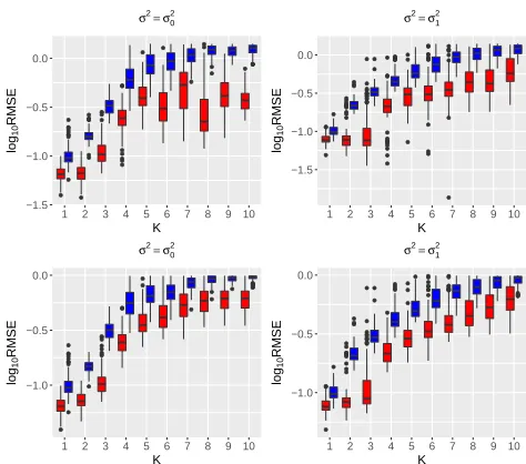
each simulation settingN = 100times independently. The estimation quality of an estimatorφbfor an eigenfunctionφ is quantified by the Monte Carlo root mean squared error (RMSE), defined byRMSE(φb) = N1 P
N
r=1kφb(r)−φkL2, while for an estimator Pb of the projection P, the Monte Carlo RMSE is given by RMSE(Pb) = N1 P
N
r=1kPb(r)−
Pk∞, whereφb(r)andPb(r)are the estimates produced in the
rth simulation replication. The results, shown in Figure 1 and 2, suggest that the multiscale approach produces better estimation quality for eigenfunctions and projections, with more prominent advantage when data exhibit a multiscale feature, such as in the case ofσ2(t) =σ20(t).
We apply multiscale FPCA to analyze the brain mi-crostructure in the corpus callosum of healthy subjects and patients with multiple sclerosis (MS). MS is a common demyelinating disease that is often caused by immune-mediated inflammation. More precisely, demyeli-nation refers to damage to myelin, an insulating material that covers nerve cells, protects axons and helps nerve sig-nal to travel faster. Patient with MS suffer from demyelina-tion that occurs in the white matter of the brain and can lose mobility or even cognitive function (Jongen, Ter Horst, and Brands 2012). Myelin damage in the brain can be examined by diffusion tensor imaging (DTI), which produces high-resolution images of white matter tissues by tracing water diffusion within the tissues. Fractional anisotropy of water diffusion can be determined from DTI and evaluated in rela-tion to MS (Ibrahim et al. 2011).
● ● ● ● ● ● ● ● ● ● ● ● ● ● ● ● ● ● ● ● ● ● ● ● ● ● ● ● ●● ● ● ●● −1.2 −0.8 −0.4 0.0
1 2 3 4 5 6 7 8 9 10
K
lo
g10
RMSE
σ2= σ
0 2 ● ● ● ● ● ● ● ● ● ● ● ● ● ● ● ● ● ● ● ● ● ● ● ● ● ● ● ● ● ● ● ● ● ● ● ● ● ●● ● ● ● ● ● −1.0 −0.5 0.0
1 2 3 4 5 6 7 8 9 10
K
lo
g10
RMSE
σ2= σ
1 2 ● ● ● ● ● ● ● ● ● ● ● ● ● ● ● ● ● ●● ● ● ● ● ● ● ● ● ● ● ● ● ●●●●●● ●●●● ●●●●●●●●●● −0.9 −0.6 −0.3 0.0
1 2 3 4 5 6 7 8 9 10
K
lo
g10
RMSE
σ2= σ
0 2 ● ● ● ● ● ● ● ● ● ● ● ● ● ● ● ● ● ● ● ● ● ● ● ● ● ● ● ● ● ● ● ● ● ● ● ● ● ●●●●●●●●●● ●●●●●●●●●●● −1.00 −0.75 −0.50 −0.25 0.00
1 2 3 4 5 6 7 8 9 10
K
lo
g10
RMSE
σ2= σ
1 2
Figure 1:log10(RMSE)of the multiscale (red) and
single-scale (blue) estimators for the first 10 eigenfunctions (top panels) and projection (bottom panels) onto the firstk lead-ing components fork= 1,2, . . . ,10forn= 50.
● ● ● ● ● ● ● ● ● ● ● ● ● ● ● ● ● ● ● ● ● ● ● ● ● ● ● ● ● ● ● ● ● ● ● ● ● ● ● ● −1.5 −1.0 −0.5 0.0
1 2 3 4 5 6 7 8 9 10
K
lo
g10
RMSE
σ2= σ
0 2 ● ● ● ● ● ● ● ● ● ● ● ● ● ● ●● ● ● ● ● ● ● ● ● ● ● ● ● ● ● ● ● ● ● ● ● ● ● ● ● ● ● ● ● ● ● ● ● ● ● ● ● ● ● ● ● ● ● ● ● ● ● ● ● ● ● ● ● ● ● ● ● ● ● ● −1.5 −1.0 −0.5 0.0
1 2 3 4 5 6 7 8 9 10
K
lo
g10
RMSE
σ2= σ
1 2 ● ● ● ● ● ● ● ● ● ● ● ● ● ● ● ● ● ● ● ● ● ● ● ● ● ● ● ●●●●●●●● −1.0 −0.5 0.0
1 2 3 4 5 6 7 8 9 10
K
lo
g10
RMSE
σ2= σ
0 2 ● ● ● ● ● ● ● ● ● ● ● ● ● ● ● ● ● ● ● ● ● ● ● ● ● ● ● ● ● ● ● ● ● ● ● ● ● ● ● ● ● ● ● ● ● ● ● ● ● ● ● ● ● ● ● ● ● ● ● ● ● ● ● ● −1.0 −0.5 0.0
1 2 3 4 5 6 7 8 9 10
K
lo
g10
RMSE
σ2= σ
1 2
Figure 2:log10(RMSE)of the multiscale (red) and
0 20 40 60 80
0.3
0.4
0.5
0.6
0.7
0.8
Tract Location
Fr
actional Anisotrop
y
0 20 40 60 80
0.004
0.006
0.008
Tract Location
V
ar
iance
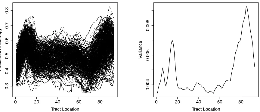
Figure 3: Left panel: fractional anisotropy profile of 382 subjects. Right panel: empirical variance function of fractional anisotropy profile.
The DTI dataset we used in the following analysis was collected at Johns Hopkins University and the Kennedy-Krieger Institute. It consists of data from n1 = 340 MS
patients and n2 = 42 healthy subjects. All fractional
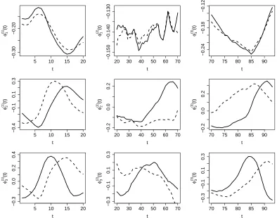
anisotropy profiles are recorded on a common grid of 93 points, as shown in the left panel of Figure 3. It seems that these profiles have larger variance at both ends relative to that in the middle. This is confirmed by the cross-sectional variance that is plotted in the right panel in Figure 3. We see that the variance function can be divided into three regions, including[0,20],[20,70]and[70,93], with relatively small variance density at[20,70]. This motivates us to apply the proposed multiscale FPCA on these regions separately. The first three estimated eigenfunctions of each region are shown in Figure 4, as well as the first three single-scale eigenfunc-tions. For comparison, the restriction of these single-scale eigenfunctions to each region is normalized to unitL2norm.
We observe that both the multiscale FPCA and single-scale FPCA yield similar results for the first principal component on each region, but differ substantially for the second and third components. For example, the first principal compo-nent on the region[20,70]is almost a straight line, which can be interpreted as a size component, i.e., subjects with a pos-itive score have larger fractional anisotropy than an average subject on locations between 20 and 70. However, for the second component, the multiscale analysis is able to capture additional features of the data on the region[20,70], while the single-scale analysis still yields almost a straight line that is similar to the depiction of its first component within that region. This agrees with our analysis in Section 2: as fractional anisotropy has low variance density on[20,70], single-scale FPCA prioritizes other regions.
It is of interest to see whether the additional patterns un-covered by MFPCA are useful for subsequent analysis, such
as predicting MS status based on fractional anisotropy. To answer this question, we study classification of MS patients and healthy subjects using a random forest classifier based on the scores derived from the firstKprincipal components. To account for the imbalance of the data, we adopt a sim-ple undersampling strategy to train the classifier as follows. We randomly sample42subjects among all 342 MS patients without replacement, and combine those data with the data from the 42 healthy subjects to form a new dataset, which we then randomly divide into two equal halves. The classifier is trained on one half, while the correct classification rate is computed on the other half. We repeat the above procedure
100times independently for eachK = 1,2, . . . ,12, where
12 is the number of components required to explain over 95% of the variance of the data. In reality,Kcould be de-termined by cross-validation or BIC criterion. We also com-pare the proposed method to wavelet transformation which is capable of localizing signals in time domain. Specifically, each fractional anisotropy profile is represented by a set of coefficients with respect to Daubechies’ least asymmetric wavelets (Daubechies 1992), and wavelet coefficients are fed into a random forest classifier. Different vanishing mo-ments are considered, namely, from db1 to db6. Roughly speaking, wavelets of more vanishing moments can repre-sent more complex function with a sparser set of wavelet coefficients.
5 10 15 20
−0.30
−0.20
t
φ1
(1
) (t
)
20 30 40 50 60 70
−0.150
−0.140
−0.130
t
φ1
(2
) (t
)
70 75 80 85 90
−0.24
−0.18
−0.12
t
φ1
(3
) (t
)
5 10 15 20
−0.4
−0.1
0.1
0.3
t
φ2
(1
) (t
)
20 30 40 50 60 70
−0.2
0.0
0.2
t
φ2
(2
) (t
)
70 75 80 85 90
−0.2
0.0
0.2
t
φ2
(3
) (t
)
5 10 15 20
−0.3
0.0
0.2
0.4
t
φ3
(1
) (t
)
20 30 40 50 60 70
−0.3
−0.1
0.1
0.3
t
φ3
(2
) (t
)
70 75 80 85 90
−0.3
−0.1
0.1
0.3
t
φ3
(3
) (t
)
Figure 4: The first 3 principal components of each partition by multiscale FPCA (solid) and single-scale (dashed) FPCA.
when K ≤ 3. A possible explanation for the observation that the multiscale method performs worse when K = 3
is that the third multiscale principal component might not be strongly related to MS status. In such case, including the component in the model does not reduce prediction bias, but increases prediction variability and thus reduces the correct classification rate.
As high-order components come into play, in particular when the fifth componentφ(3)2 , the sixth componentφ(2)2 and the seventh componentφ(1)3 are included, the advantage of MFPCA becomes more prominent. In contrast, for single-scale FPCA, the classification performance barely improves when more principal components are added. This demon-strates that MFPCA is able to discover useful features that might not be captured by single-scale FPCA in regions of low variance density. The MFPCA method also outperforms the wavelet method, likely due to the fact that principal components derived from MFPCA are innately data-driven, while wavelet bases are not. Such data-driven feature al-lows a parsimonious representation of functional data and is attractive in practice. For instance, in the above simulated functional data, on average 12 principal components are suf-ficient to account for 95% of variation of data, while over 50 wavelets are required to achieve a similar level of represen-tation.
Table 1: Correct classification rates of the random forest classifier trained on wavelet basis coefficients, multiscale principal component scores and single-scale principal com-ponent scores, respectively.
K 1 2 3 4 5 6
Multiscale 66.2 71.0 69.9 70.5 72.9 73.4 Single-scale 64.7 69.8 70.5 69.8 70.7 70.9
K 7 8 9 10 11 12
Multiscale 74.5 73.5 73.9 72.5 72.8 72.6
Single-scale 71.1 70.9 71.1 69.5 69.7 69.9
db1 db2 db3 db4 db5 db6
5
Concluding Remark
We have presented a multiscale FPCA method for functional data and demonstrated that it is numerically superior to its single-scale counterpart and the well known wavelet trans-formation, thanks to its data-driven nature and the ability to localize signals in time domain. It is worth of noting that while principal component scores from the same segment are uncorrelated, those from different segments could be cor-related. Such correlation indeed accounts for the correlation structure among different segments. This is distinct from block-diagonal structures where functional data from differ-ent segmdiffer-ents are uncorrelated or even independdiffer-ent for Gaus-sian processes. It is also of interest to apply the proposed MFPCA method to machine learning tasks other than clas-sification, such as regression and clustering, which is one of our future research topics.
Acknowledgments
Dr. Zhu’s work was partially supported by NIH grants MH086633 and MH116527.
References
Besse, P., and Ramsay, J. O. 1986. Principal components analysis of sampled functions. Psychometrika51(2):285– 311.
Chen, K., and Lei, J. 2015. Localized functional princi-pal component analysis.Journal of the American Statistical
Association110:1266–1275.
Daubechies, I. 1992. Ten Lectures on Wavelets. CBMS-NSF Regional Conference Series in Applied Mathematics. SIAM.
Dauxois, J.; Pousse, A.; and Romain, Y. 1982. Asymp-totic theory for the principal component analysis of a vector random function: some applications to statistical inference.
Journal of Multivariate Analysis12(1):136–154.
Ferraty, F., and Vieu, P. 2006. Nonparametric Functional
Data Analysis: Theory and Practice. New York:
Springer-Verlag.
Frick, K.; Munk, A.; and Sieling, H. 2014. Multiscale change-point inference. Journal of the Royal Statistical
So-ciety: Series B (Statistical Methodology)76:495–580.
Ghebreab, S.; Smeulders, A.; and Adriaans, P. 2008. Pre-dicting brain states from fmri data: Incremental functional principal component regression. In Platt, J. C.; Koller, D.; Singer, Y.; and Roweis, S. T., eds.,Advances in Neural
In-formation Processing Systems 20. Curran Associates, Inc.
537–544.
Hall, P.; M¨uller, H. G.; and Wang, J. L. 2006. Properties of principal component methods for functional and longitudi-nal data alongitudi-nalysis.The Annals of Statistics34:1493–1517. Hsing, T., and Eubank, R. 2015. Theoretical Foundations of Functional Data Analysis, with an Introduction to Linear
Operators. Wiley.
Ibrahim, I.; Tintera, J.; Skoch, A.; F., J.; P., H.; Martinkova, P.; Zvara, K.; and Rasova, K. 2011. Fractional anisotropy and mean diffusivity in the corpus callosum of patients with
multiple sclerosis: the effect of physiotherapy. Neuroradiol-ogy53(11):917–926.
Jongen, P.; Ter Horst, A.; and Brands, A. 2012. Cog-nitive impairment in multiple sclerosis. Minerva Medica
103(2):73–96.
Li, Y., and Hsing, T. 2010. Uniform convergence rates for nonparametric regression and principal component anal-ysis in functional/longitudinal data.The Annals of Statistics
38:3321–3351.
Lin, Z.; Wang, L.; and Cao, J. 2016. Interpretable functional principal component analysis. Biometrics72(3):846–854. Mas, A., and Ruymgaart, F. 2015. High-dimensional prin-cipal projections. Complex Analysis and Operator Theory
9(1):35–63.
Niu, Y. S., and Zhang, H. 2012. The screening and rank-ing algorithm to detect DNA copy number variations. The
Annals of Applied Statistics6(3):1306–1326.
Polzehl, J., and Spokoiny, V. G. 2006. Propagation-separation approach for local likelihood estimation.Probab.
Theory Relat. Fields135:335–362.
Ramsay, J. O., and Silverman, B. W. 2005.Functional Data
Analysis. Springer Series in Statistics. New York: Springer,
2nd edition.
Rao, C. R. 1958. Some statistical methods for comparison of growth curves. Biometrics14(1):1–17.
Rice, J. A., and Silverman, B. W. 1991. Estimating the mean and covariance structure nonparametrically when the data are curves. Journal of the Royal Statistical Society. Series B
53(1):233–243.
Silverman, B. W. 1996. Smoothed functional principal com-ponents analysis by choice of norm.The Annals of Statistics
24(1):1–24.
Spokoiny, V., and Vial, C. 2009. Parameter tuning in point-wise adaptation using a propagation approach. Ann. Statist.
37:2783–2807.
Yao, F.; M¨uller, H. G.; and Wang, J.-L. 2005. Functional data analysis for sparse longitudinal data. Journal of the
American Statistical Association100:577–590.
Zhang, X., and Wang, J. L. 2016. From sparse to dense func-tional data and beyond. The Annals of Statistics 44:2281– 2321.
Zhu, H.; Fan, J.; and Kong, L. 2014. Spatially varying coef-ficient models with applications in neuroimaging data with jumping discontinuity. Journal of American Statistical