Please cite this article as: J. Arkat, R. Jafari, Network Location Problem with Stochastic and Uniformly Distributed Demands, International Journal of Engineering (IJE), TRANSACTIONS B: Applications Vol. 29, No. 5, (May 2016) 654-662
International Journal of Engineering
J o u r n a l H o m e p a g e : w w w . i j e . i rNetwork Location Problem with Stochastic and Uniformly Distributed Demands
J. Arkat*, R. Jafari
Department of Industrial Engineering, University of Kurdistan, Kurdistan, Iran
P A P E R I N F O
Paper history:
Received 08 February 2016
Received in revised form 06 March 2016 Accepted 14 April 2016
Keywords: Network Location Congested Facilities Distributed Demand Queueing Models Metaheuristic Algorithms
A B S T R A C T
This paper investigates the network location problem for single-server facilities that are subjected to congestion. On each network edge, customers are uniformly distributed, and their requests for service are assumed to be generated according to a Poisson process. A number of facilities are to be selected from a number of candidate sites, and a single server is located at each facility with exponentially distributed service times. Using queueing analysis, we develop a mixed integer mathematical model to minimize the total travel and the average waiting times for customers. For evaluation of the validity of the proposed model, a numerical example is solved and analyzed using GAMS software. In addition, since the proposed problem is NP-hard, two metaheuristic algorithms including a genetic algorithm and a simulated annealing algorithm are developed and applied for large-size problems.
doi: 10.5829/idosi.ije.2016.29.05b.09
1. INTRODUCTION1
Facility location models can be categorized into two main categories based on the type of the servers; customer-to-server models (as for primary health care centers, automatic teller machines (ATM), and proxy servers), and server-to-customer models (as for emergency facilities such as ambulance, police and fire stations). In another classification, models are categorized based on the absence or presence of congestion at the facilities. In the first category, it is assumed that each customer is immediately served upon his or her arrival and therefore, queues do not form at servers. The basic location models such as covering models (e.g., [1]), p-median (e.g., [2, 3]) and p-center models belong to this category. Location models for congested facilities fall in the second category in which service times are considered not to be negligible compared to inter-arrival times. Therefore, each customer may has to wait in a queue upon his or her arrival.
Location models for congested facilities are classified based on the primary assumptions made about server queues, such as type of arrival and service
1*
Corresponding Author Email:[email protected] (J. Arkat)
processes, number of servers, capacity of facilities and so on. Commonly, it is assumed that the arrival process for each server is a Poisson (that is, the inter-arrival times are exponentially distributed). Another assumption, which is not as common as the previous one, is that service times for each server follow exponential distribution. However, some researchers have considered service times as a general distribution or as deterministic quantities. In the case of the number of servers in each facility, most location models are single-server models, and, therefore, M/M/1, M/D/1 and M/G/1 are widespread queueing models in the field (e.g., [4-8]). Compared to single-server models, those that allow multiple servers in each facility are limited and usually concerned with exponentially distributed service times (that is, the M/M/c queue); e.g., [9-11]. There are only a few studies which have tended to consider non-exponential distributions for service times [12-14].
customers arrive randomly at an ATM, and if the facility is idle upon their arrival, they will be served immediately. Otherwise, they will join the queue or leave [17]. These two applications are just examples of the many application areas that have been mentioned in the literature. Boffey et al. [18] have provided a complete review of location models for congested facilities with immobile servers. In the following, we review the research addressing the location problem for congested facilities with immobile servers.
Wang et al. [19] have considered the problem of locating facilities that are modeled as M/M/1 queuing systems. Each customer travels to the closest facility and joins the queue if the expected waiting time is below a certain threshold. The objective function is to minimize the sum of the total traveling and the average waiting times for all customers. Berman and Drezner [20] have extended the aforementioned model by allowing more than one server to be located at each facility and thus employing M/M/c queuing model. Motivated by applications to locating servers in communication networks and ATMs, Wang et al. [17] have presented several models for the facility location problem subjected to congestion. Berman et al. [21] have developed a model similar to that of Wang et al. [19], except that they have considered the demand lost due to congestion or insufficient coverage. The objective function of this model was to minimize the number of facilities. Boffey et al. [22] have considered the location problem for a single facility that operates as an M/Er/1/N queuing system. Marianov et al. [14] have considered an extension to the previous model for M/Er/c/N systems along with a constraint on the probability of a customer being lost. Pasandideh and Niaki [23] have proposed a bi-objective facility location problem within M/M/1 queuing framework for the p-median problem. The authors have solved the proposed problem using a genetic algorithm (GA) in which the desirability function technique has been utilized.
When the number of customers on each edge is large (for example, customers of ATMs and shopping malls, which are dispersed over the streets), three alternatives can be considered: a) treating each customer as a single point on the network that can make the model unsolvable even for small instances, b) considering a single point on each edge as the representative for an entire edge and assigning all customer demands to that point and c) considering a continuous distribution to represent demands on each edge. A common assumption in all previous studies is to consider locations of customers as known points on the network. This assumption may represent some real-world situations, or it may simply mean that all demands on an edge are generated from a single point. In the second case, although the assumption facilitates the modelling process, it has a serious drawback: in the optimal solution, each demand point (that, in fact, corresponds
to an edge) is assigned to a single server. Therefore, all customers on the edge have to travel to this server. It is not difficult to see that this is usually in contrast to the common assumption that each customer is assigned to the closest facility. To overcome this difficulty, instead of considering representative points for edges, we assume that customers’ demands are distributed uniformly along the network edges. In other words, it is assumed that each edge has a known demand rate that is a function of its length and the local congestion. Each customer on a specific edge travels to the facility closest to it, and therefore, two customers on a single edge may travel to different facilities.
The rest of the paper is organized as follows. In the next section, the facility location problem for congested facilities with immobile servers is described in detail and then modeled as a mixed linear integer program. Since the investigated problem is NP-hard, two metaheuristic algorithms are presented in Sections 3 and 4. In order to evaluate the performance of the proposed algorithms, we analyze a number of numerical examples in Section 5. Finally, the conclusions and some directions for future research are presented in Section 6.
2. PROBLEM DESCRIPTION
The formal description of the problem is as follows. Let
,
G V E be an undirected graph with set
1, , , 2 n
V v v v of vertices and set E V V of edges. Some vertices represent potential locations for setting up a predefined number of servers in such a way that at most one server is located at each candidate site. All servers have the same and a known service rate. The occurrence process of demands on each edge is supposed to be a homogeneous spatial Poisson process in R ; that is, demand is uniformly distributed along 1
each edge, and times between consecutive demands on the edge are exponentially distributed at a known rate. This stochastic process is similar to the spatial renewal process defined by Baron et al. [24] for the continuous location problem.
It is obvious that the demand rate for a portion of an edge is proportional to its length. For simplicity, we state the length of an edge or a portion of an edge as the travel time for the corresponding distance. The problem is to select a predetermined number of servers and to assign all demands on the network edges in such a way that the sum of the total travel time and the average waiting time is minimized. The assumptions are summarized below:
Customers travel to the closest facility. All customers travel at the same speed.
Balking (that is, the reluctance to join a queue upon arrival) and reneging (that is, the reluctance to remain in queue after joining) are not permitted. The average waiting time at each server is less than
a specified threshold.
The notation of the proposed model is defined as follows:
Sets and Indices
V Set of network vertices
,
v v Indices for vertices
J Set of candidate sites
,
j j Indices for candidate sites
E Set of network edges
Parameters
vv
d Travel time of edge
v v, vv Demand rate of edge
v v, vjt Shortest time between vertex v and candidate site j
Service rate for each server
p Number of facilities
max
w Upper bound on the average waiting time at
each facility
M A large positive number
Decision variables
j
y Binary variable that is equal to one if a facility
is located at candidate site j and zero otherwise
vj
x Binary variable that is equal to one if vertex v
is assigned to the facility located at candidate site j and zero otherwise
j
w Average waiting time for the facility located at
candidate site j
j
Demand rate for the facility located at
candidate site j
'
vv jj
b Travel time between vertex v and partitioning point of edge
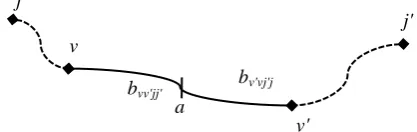
v v, if vertices v and v are respectively assigned to the facilities located at candidate sites j and jIn view of the aforementioned assumptions and notation, the proposed problem is modeled as follows. To start with, consider edge
v v, and two facilities located at candidate sites j and j (as shown in Figure 1). If all customers on this edge have to travel to a facility only through one of its endpoints, the total travel time to arrive at this endpoint is obtained as follows:0 2
vv d
vv
vv vv
vv
d x
T dx
d
(1)Figure 1. Dividing an edge into two partitions
Due to the first assumption, some customers on each edge travel to one vertex, while the others may go to the other vertex. If a partitioning point is determined, each edge is divided into two segments. Figure 1 shows an example of such a partitioning point (point a) for edge
v v, , in which customers on sub-edges
v a, and
a v,
travel to vertices v and v, respectively. It isobvious that if one of these sub-edges has a length of zero, it means that all customers travel to one vertex.
If the closest facilities for vertices v and v are respectively located at vertices j and j, then bvv jj , and hence the partitioning point for this edge, is calculated using the following equality:
1
1
2
vv jj vv v j vj vj v j
b d t t if x x (2)
In order to obtain the total travel time for all customers, consider edge
v v, . The length of sub-edge
v a, isvv jj
b , and hence, the average number of customers (demands) on this sub-edge per unit of time is
vvbvv jj dvv
. Each customer in this interval travels first to vertex v and then to the facility closest to this vertex. Therefore, T1, as the total travel time for all customers per unit of time, is calculated as follows:
1
, 2
vv jj vv vv jj vj vj v j j J j J v v E vv
b b
T t x x
d
(3)For calculation of the average waiting time at each facility, the queue discipline should be analyzed in advance. Due to the third assumption made before, demand occurrence (call for service) on each edge follows a Poisson process. After a demand occurrence, the corresponding customer has to travel a uniformly distributed distance to arrive at the closest facility. Such travel times make the arrival process different from the occurrence process. However, it can be shown that the arrival process at each facility is Poisson (see [25] for proof), and hence, each server behaves just as an M/M/1 queue. Now, it is straightforward to calculate the average waiting time for each server and hence the total average waiting time for all customers. The total arrival rate for server j can be calculated as follows:
j
j' v
v' a
bvv'jj'
,
vv jj vv
j vj v j
j J v v E vv
b x x d
(4)and the average waiting time is: 1 j j w (5)
Therefore, the total average waiting time for all customers is calculated as follows:
2
j
j J j
T
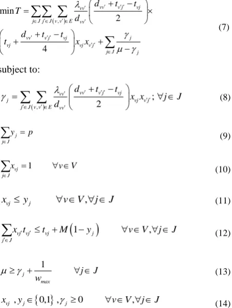
(6)Now, the two parts of the objective function have been calculated, and we arrive at the following model:
,
min
2
4
vv v j vj vv
j J j J v v E vv
vv v j vj j
vj vj v j
j J j
d t t T
d
d t t
t x x
(7) subject to: , ; 2vv v j vj vv
j vj v j
j J v v E vv
d t t
x x j J d
(8)j j J y p
(9) 1 vj j Jx v V
(10), vj j
x y v V j J (11)
1
,vj vj vj j
j J
x t t M y v V j J
(12) 1 j max j J w (13)
, 0,1 , 0 ,
vj j j
x y v V j J (14)
In the above model, Equation (7) is the objective function, which consists of two parts: the total travel time and the total average waiting time for all customers. The first term of this objective function is obtained through replacement of bvv jj in Equation (3) by its equivalent quantity from Equation (2). In a similar manner, the second part of the objective function is obtained from Equation (2) and Equation (4). The total arrival rate for each facility is calculated using Equation (8). This constraint imposes that if a server is not located at a candidate site, the arrival rate corresponding to this location will be zero. Constraint (9) determines the number of facilities. Constraints (10)
and (11) together ensure that each network vertex is assigned to a facility, and constraint (12) guarantees that this assignment is done to the closest facility. An appropriate value for M in this constraint is
max tvv, , v v A . Constraint (13) ensures that the average waiting time for each facility does not exceed the threshold wmax. Finally, the last constraint defines the domains of the decision variables. Although the proposed model is nonlinear due to the multiplication of two binary variables in the objective function and constraint (8), and also the presence of a decision variable in the denominator of the second part of the objective function, it can be changed to a linear mixed integer model. The proposed model can be solved using linear integer optimization software for small-size problems. In order to verify the validity of the proposed model, we present and solve a small numerical example.
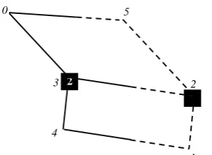
The numerical example presented in this section is a small instance of a network consisting of six vertices, seven edges, four candidate sites and two facilities. The service rate for each server is 60 customers per hour, and the maximum permitted average waiting time is 40 min. The network is illustrated in Figure 2, in which the candidate sites are shown as squares. In addition, Table 1 shows the travel times and demand rates for the edges. The model is solved using the optimization software GAMS (the solver CPLEX). In the optimal solution, candidate sites 1 and 2 are selected for establishing a server at each.
Figure 2. An example with six vertices and seven edges
TABLE 1. Data for the first numerical example
v v, dvv (min) vv (per min)(0,3) 2.30 11.48
(0,5) 2.18 4.36
(1,2) 1.67 0.08
(1,4) 2.48 0.12
(2,3) 2.49 12.43
(2,5) 2.75 13.77
(3,4) 1.48 2.97
Figure 3. The optimal solution for the first example
In addition, vertices 1, 2 and 5 are assigned to the server located at vertex 1, and the other vertices (that are, vertices 0, 3 and 4) are assigned to the server located at vertex 2. The optimal configuration of the network is illustrated in Figure 3, in which the dashed edges or sub-edges are assigned to server 1, and the others are assigned to server 2. The objective function in the optimal solution equals 128.30 min, which is the sum of 55.68 min as the total travel time and 72.62 min as the total average waiting time.
As we mentioned before, the proposed problem is NP-hard, and therefore, the proposed model cannot be solved optimally for large-size real-world problems. In the next two sections, we present two metaheuristic algorithms including a modified version of the genetic algorithm (GA) proposed by Alp et al. [26] and a simulated annealing (SA) algorithm.
3. GENETIC ALGORITHM
Genetic algorithms are systematic population-based search algorithms that mimic natural genetics by using procedures inspired by natural evolution, such as mutation, crossover and selection. In a GA, a population of encoded solutions (chromosomes) is evolved toward better solutions. This evolution usually starts from a randomly generated population called initial generation. In each generation, chromosomes of the current population are randomly selected based on their fitness, and modified through genetic operators to form a new population. This improvement cycle is repeated until a termination rule is met. The proposed GA is similar to the algorithm developed by Alp et al. [26] for the well-known p-median problem. The main difference lies in the procedure of calculating the fitness function for each chromosome. The proposed GA is briefly explained in the next subsections.
3. 1. Encoding and Decoding The most important issue in the design of a metaheuristic algorithm is finding an efficient encoding procedure in which each solution is represented as a string or matrix. Similar to
the p-median problem, the proposed problem can be seen as selecting p facilities from m candidate sites. Each chromosome is represented by an array of p
unique positive integers chosen from set 1, 2, , m. Genes of a chromosome represent the indices of the selected candidate sites. This encoding scheme respects all the constraints of the proposed model, except constraint (13). In other words, if an encoded string is filled by randomly selected candidate vertices, it may cause the average waiting times for some facilities to be greater than the maximum permitted average waiting time. In such cases, a penalty is associated with the fitness function. The initial population is generated based on the procedure proposed by Alp et al. [26].
Decoding is the process of transferring
chromosomes from the search space into the solution space; that is, each chromosome is converted from a string or matrix to a fitness function. In the proposed GA, the objective function value for each string is considered as its fitness. As we mentioned before, a penalty is added to the fitness values of infeasible solutions. The amount of the penalty is proportional to the maximum allowed average waiting time (that is,
max
w
), and the value of is set to 2 for numerical examples.
3. 2. Selection and Reproduction The crossover and the selection operators are the same as those reported by Alp et al. [26], and as in that paper, we do not apply a mutation operator. In the crossover operator, two chromosomes are selected randomly as parents, and an offspring is generated by taking the union of the parents’ alleles. Obviously, the produced offspring may be infeasible in the sense that its size exceeds the number of facilities. The correction process is performed through removal of extra genes, one by one and in a greedy manner. The genes that are common in both parents do not take place in the elimination. At each iteration, a gene is discarded which produces the best fitness function value (i.e., increases the fitness value by the least amount). The generated offspring then goes through a selection process. In the selection phase, an offspring that is not identical to an existing chromosome and its fitness value is better than the worst fitness value in the current population is added to the population, while the worst existing chromosome is discarded. This selection operator results in a gradual improvement of the average fitness function of the population. The algorithm terminates after observing
m p
successive iterations where the best solution has
not changed.
Although this algorithm has some basic differences from the standard GA, the numerical examples provided in Section 5 illustrate its capability in finding relatively good solutions in extremely short run times. The most
5 0
4
3 2
1 2
important obstacle in this algorithm is the elite strategy selection, in which the weakest chromosomes are always eliminated. This characteristic increases the probability of falling into local optimum traps.
4. SIMULATED ANNEALING
Simulated annealing is a structured search heuristic that was inspired by the real annealing process in the metallurgical industry. The simple structure along with high capability in escaping from being trapped into local optimums have made SA a popular metaheuristic algorithm in solving combinatorial optimization and real-world problems. SA was originally introduced by Kirkpatrick et al. [27]. Annealing is the process in which slow cooling is applied to metals to produce better-aligned, low energy-state crystallization. The optimization procedure of SA searches for a (near-) global minimum mimicking the slow cooling procedure in the physical annealing process [28].
Unlike population-based algorithms, SA is a single-solution-based algorithm; that is, it starts with a randomly generated solution. The initial solution is gradually improved using a controlled neighborhood search procedure. There are two cycles in the algorithm: an outer cycle and an inner cycle inside the outer cycle. In each iteration of the inner cycle, a neighbor solution is generated for the current solution using a local search procedure. The objective function of the new solution is then compared to that of the current solution, to determine if an improvement has been achieved. If the neighbor solution is better than the current solution, it is considered as the new current solution; otherwise, it may still be accepted as the new current solution with a specific probability. This characteristic, which is in contradiction with greedy algorithms, prevents SA from falling into local optimum traps. Each inner cycle is repeated until a certain number of neighbor solutions are generated or a prespecified number of such solutions are accepted. After the inner cycle meets the termination rule, the temperature is reduced in the outer cycle, and the inner cycle is run again. The temperature reduction process reduces the probability of accepting worse neighbor solutions. This means that while the algorithm tries to explore the whole solution space in the initial steps, it gradually focuses on the neighborhood of the global optimum solution. The outer cycle is repeated until a termination rule, which is usually set based on a freezing temperature, is met.
The most important procedure in an SA algorithm is the process of generating neighbor solutions, which significantly affects the quality of the final solution. For each solution, the neighbor solutions are defined as those solutions having a predefined maximum number of genes different from that in the current solution. The maximum number of different genes is considered to be
p 4, where p is the number of facilities. Each
neighbor solution is selected randomly from the proposed neighborhood structure. This is done through generation of r, a random number between 1 and p 4.
Then, r genes are randomly selected from the current solution string, and their alleles are altered to those that are not in the primary string. The resulting string is considered as a neighbor solution.
A number of initial parameters have to be set before the SA algorithm is run. These parameters are T0, the initial temperature, Tf, the freezing temperature, , the cooling factor, N1, the maximum number of improving neighbor solutions in an inner cycle, and
2
N , the maximum number of non-improving neighbor solutions in an inner cycle. The value of T0 is set in such a way that the probability of accepting a worse neighbor solution in the first outer cycle is more than 0.90. In a similar manner, the value of Tf is set such that the probability of accepting a worse neighbor solution in the last outer cycle is less than 0.01. The following values are found to achieve the best solutions for numerical examples: T050, Tf 0.001,0.90,
1
N m, and N2p.
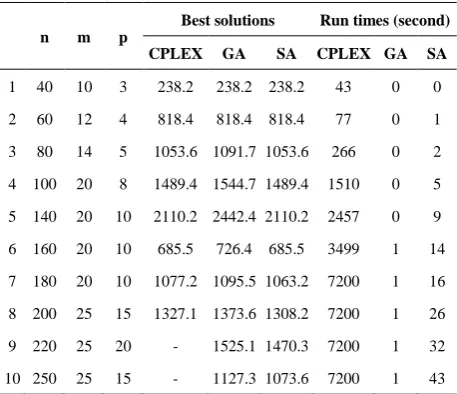
5. COMPUTATIONAL RESULTS
For evaluation and comparison of the performance of the proposed algorithms, a number of numerical examples are presented in this section. Since numerical examples are not provided in the literature, we used a random problem generating procedure. The generated instances vary from small-size problems on a 40-vertex
TABLE 2. The results for the numerical examples
n m p
Best solutions Run times (second)
CPLEX GA SA CPLEX GA SA
1 40 10 3 238.2 238.2 238.2 43 0 0
2 60 12 4 818.4 818.4 818.4 77 0 1
3 80 14 5 1053.6 1091.7 1053.6 266 0 2
4 100 20 8 1489.4 1544.7 1489.4 1510 0 5
5 140 20 10 2110.2 2442.4 2110.2 2457 0 9
6 160 20 10 685.5 726.4 685.5 3499 1 14
7 180 20 10 1077.2 1095.5 1063.2 7200 1 16
8 200 25 15 1327.1 1373.6 1308.2 7200 1 26
9 220 25 20 - 1525.1 1470.3 7200 1 32
network to relatively large-size problems on a 250-vertex network. The mathematical model is solved for each instance using CPLEX solver of GAMS software. In addition, the proposed metaheuristic algorithms are coded in Microsoft Visual C# 2008. All the programs are run on a PC with 4 GB RAM and Core i3 2.27 GHz & 2.26 GHz CPU. The proposed GA and SA are implemented 10 times for each problem instance, and the best solution is reported. The maximum run time for CPLEX is considered two hours. The results are summarized in Table 2.
As can be seen in Table 2, CPLEX has found the global optimum for the first six instances. In examples 7 and 8, the software has not achieved the global optimum in two hours, and hence, the best solution is reported. Moreover, for problems 9 and 10, CPLEX has not found any feasible solutions. The table indicates that the proposed SA has achieved the best solutions in all the problem instances. The proposed GA has considerably shorter run times for all the examples. On the other hand, its performance in terms of the quality of the final solutions is not as good as the results obtained by the SA. Since the proposed problem is a design problem, the run time of the solution algorithm is not as important as the quality of the final solution. In other words, in comparison with the solution procedures for such problems, the quality of the final solution should be considered as the key criterion. The short run times for the proposed GA make the algorithm a good candidate for hybridization with other metaheuristic algorithms.
6. CONCLUSION
We proposed a new mathematical model for the network location problem of congested facilities with immobile servers. We assumed that the locations of customers (as sources for demands) are uniformly
distributed along the network edges, as a
straightforward extension to the recent studies. As compared to the common assumption of demand points in the previous works, although the assumption of uniformly distributed demands has resulted in a complex mathematical model, it copes well with real-world situations. Based on this idea, the problem is to select a predefined number of facilities from a number of candidate sites and to assign network edges to them. We assumed that each customer travels to his or her closest facility, which is a usual assumption. At each facility, a single server is located with exponentially distributed service times. Furthermore, we supposed that the occurrence process for demands on each edge is Poisson. Based on these assumptions, we proved that each server acts as an M/M/1 queue. The objective function of the proposed model was the minimization of the sum of the total travel and the average waiting times
for all customers. The problem was formulated as a mixed integer linear model. Moreover, since the problem is NP-hard, we developed two metaheuristic algorithms (that is, GA and SA) to solve the problem for large-size instances. A number of numerical examples were used for evaluation of the performance of the proposed algorithms. The results demonstrate the explicit preference of the SA over the GA.
The proposed problem along with the developed model have the ability to open a new study area in the field of location problems for congested facilities. We believe that considering the following assumptions provides interesting fields for future research:
General distribution service times (M/G/1 queue model for each facility).
Multiple servers at each facility (M/M/C queue for each facility).
Limited capacity for each facility (M/M/1/K and M/M/C/K queue models).
Impatient customers (balking, reneging and jockeying).
The main difficulty in modeling the above extensions is the relatively complex form of the average waiting time (wj). Although a closed form exists for wj for all of these cases, the procedure of linearization will be challenging or perhaps impossible.
In the proposed model, it has been assumed that each customer is assigned to his or her closest facility. While this assumption is common in related studies, in many real-world applications, customers tend to travel to the ―best‖ facility instead of the closest one. The ―best‖ facility for a customer can be defined as the facility with the shortest sum of travel and waiting times for the customer. However, this new assumption would result in a more complex mathematical model (particularly, in defining partitioning points for edges).
7. REFERENCES
1. Bashiri, M. and Rezanezhad, M., "A reliable multi-objective p-hub covering location problem considering of p-hubs capabilities",
International Journal of Engineering-Transactions B:
Applications, Vol. 28, No. 5, (2015), 717-729.
2. Tavakkoli-Moghaddam, R., Gholipour-Kanani, Y. and
Shahramifar, M., "A multi-objective imperialist competitive algorithm for a capacitated single-allocation hub location problem", International Journal of Engineering-Transactions
C: Aspects, Vol. 26, No. 6, (2013), 605-612.
3. Ghodratnama, A., Tavakkoli-Moghaddam, R. and Baboli, A.,
"Comparing three proposed meta-heuristics to solve a new p-hub location-allocation problem", International Journal of
Engineering-Transactions C: Aspects, Vol. 26, No. 9, (2013),
1043-1058.
4. Berman, O., Larson, R. C. and Chiu, S. S., "Optimal server location on a network operating as an M/G/1 queue",
5. Batta, R., "Single server queueing-location models with rejection", Transportation Science, Vol. 22, No. 3, (1988), 209-216.
6. Batta, R., Larson, R. C. and Odoni, A. R., "A single‐server priority queueing‐location model", Networks, Vol. 18, No. 2, (1988), 87-103.
7. Batta, R., "A queueing-location model with expected service time dependent queueing disciplines", European Journal of
Operational Research, Vol. 39, No. 2, (1989), 192-205.
8. Jamil, M., Baveja, A. and Batta, R., "The stochastic queue center problem", Computers & Operations Research, Vol. 26, No. 14, (1999), 1423-1436.
9. Marianov, V. and Serra, D., "Probabilistic, maximal covering location—allocation models forcongested systems", Journal of
Regional Science, Vol. 38, No. 3, (1998), 401-424.
10. Marianov, V. and Serra, D., "Hierarchical location–allocation
models for congested systems", European Journal of
Operational Research, Vol. 135, No. 1, (2001), 195-208.
11. Marianov, V. and Serra, D., "Location–allocation of multiple-server service centers with constrained queues or waiting times",
Annals of Operations Research, Vol. 111, No. 1-4, (2002),
35-50.
12. Khalili, S., ZareMehrjerdi, Y., Fallahnezhad, M. and Mohammadzade, H., "Hotel location problem using erlang queuing model under uncertainty", International Journal of
Engineering-Transactions C: Aspects, Vol. 27, No. 12, (2014),
1879-1887.
13. Marianov, V. and Serra, D., "Location models for airline hubs
behaving as M/D/c queues", Computers & Operations
Research, Vol. 30, No. 7, (2003), 983-1003.
14. Marianov, V., Boffey, T. B. and Galvao, R. D., "Optimal location of multi-server congestible facilities operating as queues", Journal of the Operational Research Society, Vol. 60, No. 5, (2009), 674-684.
15. Li, B., Golin, M. J., Italiano, G. F., Deng, X. and Sohraby, K., "On the optimal placement of web proxies in the internet", in INFOCOM'99, Eighteenth Annual Joint Conference of the IEEE Computer and Communications Societies, Vol. 3, (1999), 1282-1290.
16. Gautam, N., "Performance analysis and optimization of web
proxy servers and mirror sites", European Journal of
Operational Research, Vol. 142, No. 2, (2002), 396-418.
17. Wang, Q., Batta, R. and Rump, C. M., "Facility location models for immobile servers with stochastic demand", Naval Research
Logistics (NRL), Vol. 51, No. 1, (2004), 137-152.
18. Boffey, B., Galvao, R. and Espejo, L., "A review of congestion models in the location of facilities with immobile servers",
European Journal of Operational Research, Vol. 178, No. 3,
(2007), 643-662.
19. Wang, Q., Batta, R. and Rump, C. M., "Algorithms for a facility location problem with stochastic customer demand and immobile servers", Annals of Operations Research, Vol. 111, No. 1-4, (2002), 17-34.
20. Berman, O. and Drezner, Z., "The multiple server location problem", Journal of the Operational Research Society, Vol. 58, No. 1, (2007), 91-99.
21. Berman, O., Krass, D. and Wang, J., "Locating service facilities to reduce lost demand", IIE Transactions, Vol. 38, No. 11, (2006), 933-946.
22. Boffey, B., Galvao, R. D. and Marianov, V., "Location of single-server immobile facilities subject to a loss constraint",
Journal of the Operational Research Society, Vol. 61, No. 6, (2010), 987-999.
23. Pasandideh, S. H. R. and Niaki, S. T. A., "Genetic application in a facility location problem with random demand within queuing framework", Journal of Intelligent Manufacturing, Vol. 23, No. 3, (2012), 651-659.
24. Baron, O., Berman, O. and Krass, D., "Facility location with stochastic demand and constraints on waiting time",
Manufacturing & Service Operations Management, Vol. 10, No. 3, (2008), 484-505.
25. Mirasol, N. M., "Letter to the editor-the output of an M/G/∞ queuing system is poisson", Operations Research, Vol. 11, No. 2, (1963), 282-284.
26. Alp, O., Erkut, E. and Drezner, Z., "An efficient genetic algorithm for the p-median problem", Annals of Operations
Research, Vol. 122, No. 1-4, (2003), 21-42.
27. Kirkpatrick, S. and Vecchi, M. P., "Optimization by simmulated annealing", Science, Vol. 220, No. 4598, (1983), 671-680.
Network Location Problem with Stochastic and Uniformly Distributed Demands
J. Arkat, R. Jafari
Department of Industrial Engineering, University of Kurdistan, Kurdistan, Iran
P A P E R I N F O
Paper history:
Received 08 February 2016
Received in revised form 06 March 2016 Accepted 14 April 2016
Keywords: Network Location Congested Facilities Distributed Demand Queueing Models Metaheuristic Algorithms
ديكچ ه
ىاکه ِلأسه ِلاقه يیا رد ِکبش یبای
تهذخ کی یاراد تلایْست یارب یا یه رارق یسررب درَه ،ماحدزا ذعتسه ُذٌّد
.دریگ
ىاوک رد ىایرتشه ُذش عیزَت تخاٌَکی ترَص ِب ِکبش یاّ
ذٌیآرف کی ساسارب ،تاهذخ یارب اًْآ تساَخرد ٍ ذًا
ایرد ،ىاساَپ یه تف تیاس زا یداذعت باختًا ،ِلأسه فذّ .دَش رارقتسا ٍ لیْست یصخشه داذعت رارقتسا یارب اذیذًاک یاّ
تهذخ کی ىاهز اب ُذٌّد نتسیس لیلحت زا ُدافتسا اب .تسا تلایْست زا کی رّ رد ییاوً عیزَت یاراد یاّ
کی ،فص یاّ
ٌِیوک یارب ِتخیهآ حیحص دذع یطخ لذه ىاهز طسَته یزاس
اّ یه ُداد ِعسَت ،ىایرتشه راظتًا ی یسررب رَظٌه ِب .دَش
مرً زا ُدافتسا اب ٍ ِئارا ،یدذع لاثه کی ،یضایر لذه تحص ٌِیْب راسفا
زاس
GAMS
یه لح ِکًآ لیلد ِب يیٌچوّ .ددرگ
ِلوجذٌچاً ،یسررب تحت ِلأسه یرَگلا کی ٍ کیتًش نتیرَگلا کی لهاش یراکتباارف نتیرَگلا ٍد ،تسا تخس یا
گٌیلًآ نت
ِیبش یه ِتفرگ راک ِب گرسب سایقه رد ِلأسه لح یارب ٍ ِعسَت ،ُذش یزاس .دَش