S
S
O
O
L
L
V
V
I
I
N
N
G
G
T
T
H
H
E
E
N
N
E
E
X
X
T
T
R
R
E
E
L
L
E
E
A
A
S
S
E
E
P
P
R
R
O
O
B
B
L
L
E
E
M
M
U
U
S
S
I
I
N
N
G
G
A
A
H
H
Y
Y
B
B
R
R
I
I
D
D
M
M
E
E
T
T
A
A
H
H
E
E
U
U
R
R
I
I
S
S
T
T
I
I
C
C
A
A
.
.
O
O
.
.
B
B
a
a
l
l
o
o
g
g
u
u
n
n
,
,
M
M
.
.
A
A
.
.
M
M
a
a
b
b
a
a
y
y
o
o
j
j
e
e
,
,
M
M
.
.
O
O
.
.
M
M
a
a
k
k
i
i
n
n
w
w
a
a
,
,
A
A
.
.
O
O
.
.
B
B
a
a
j
j
e
e
h
h
Department of Computer Science, University of Ilorin, Ilorin, Nigeria
Corresponding author: A. O. Balogun, [email protected]
ABSTRACT: The Next Release Problem is characterized by the need to determine the features that are to be included in a particular software system to make up the next release. These features are to be selected, such that users’ demands and needs are satisfied as much as possible, given a limited resources, by ensuring that the available resources are used to develop the most important features first. This work applies a hybrid of Variable Neighbourhood Search (VNS) and Tabu Search (TS) for solving bi-objective NRP, using a cost-value model for requirements. Experiments showed the hybrid metaheuristics to produce a Pareto optimal set with a controllable dynamic number of options whose score and cost value range can be controlled via parameters that can be modified without a significant effect on execution time.
KEYWORDS: Software Engineering, Search Based Software Engineering, Next Release Problem, Variable Neighbourhood Search, Tabu Search, Optimization, Multiobjectivity.
1. INTRODUCTION
A problem inevitable to software engineers and organizations that develop and maintain large and complex software to be used by some range of users, is the problem of selecting what should be in the next release of the software. The problem is characterized by users requesting for a wide range of changes (requirements) in the software, costs of meeting such requirements (time and effort) varying widely, a situation where some changes in the software will require some other prerequisite changes, users have different values to the software engineer or organization, and as such, the various requirements have to be considered in a way that customers with more value will be favoured more ([BRW01]). Software engineers need to select requirements to include in the software next release such that customers’ demands and needs are as much as possible satisfied while ensuring that budget (time and money) for the software development is not exceeded by ensuring that the available resources are used to develop the most important requirements first. This problem is called the Next Release Problem (NRP). It is very
important to the software engineers and organizations alike that this set of requirements to be fulfilled in the next release be carefully selected so as to avoid losing important customers and going over budget which could result when a wrong decision is made in selecting which requirements to actually fulfill.
Selecting an optimal set of requirements for the next release of a software is an optimization problem and it is NP-hard ([BRW01]). Various heuristics – local search algorithms like hill climbing algorithm, simulated annealing; global search algorithms like genetic algorithms; and multi-objective algorithms like ant colony optimization algorithm, pareto GA, pareto archived evolutionary strategy (PAES), non-dominated sorting genetic algorithm II (NSGA-II), have been used in literature to find high quality near optimal solutions with NSGA II giving the highest number of optimal solutions for large test cases ([D+11]).
Furthermore, the Next Release Problem (NRP) is an example of Feature Subset Selection (FSS) Problem ([B+06, ZH10, ZHL13, ZHM07, HT07]). Baker et al. ([B+06]) formulated both ranking and selection of candidate software components as a series of feature subset selection problems to which heuristics was be applied. Garcia-Torres, Garcia-Lopez, Melian-Batista, Moreno-Perez, & Moreno-Vega ([G+04]) applied a hybrid metaheuristic based on Variable Neighbourhood Search (VNS) and Tabu Search (TS) – both global search algorithms, to solving the FSS problem with the hybrid producing results with a higher reduction in the set of features than those gotten from applying genetic algorithm. This research work applies a hybrid of Variable Neighbourhood Search (VNS) and Tabu Search (TS) to solving the NRP, using a cost-value model for requirements.
2. RELATED WORKS
Metaheuristic search techniques have been quite significantly applied to software engineering problems ([HMZ09]). This is due to the fact that such software engineering problems can be readily formulated as optimization problems as they have the characteristics of requiring a balance between objectives that are conflicting and competing ([HMZ09, H+12]). This review will focus on Search Based Software Engineering (SBSE) and the previous work that has been done on applying SBSE to the various stages in the software development life cycle.
2.1. Search Based Software Engineering (SBSE)
In their paper, Harman & Jones ([HJ01]) claimed the emergence of the new field of research and practice in software engineering and coined the name Search Based Software Engineering (SBSE). They argued that most software engineering problems can be represented as search problems such that metaheuristics can be applied to find near optimal solutions to them.
The following observations are typical of software engineering problems, basically the factors that make them so suitable to be reformulated as search problems (HJ01):
1. Usual need to optimize conflicting objectives
2. Usual need to balance competing objectives 3. There are usually quite a number of possible
solutions
4. Getting a perfect answer is often impossible or impractical
5. A number of good enough solutions can be achieved
Fig. 1. Example of SBSE in requirements selection and regression testing ([H+12])
2.1.1. SBSE in Requirements Analysis and Selection
Whether or not a software system will succeed depends on how well it caters to the needs of its users in the form of software requirements.
Fig. 2. Traditional engineering fields vs software engineering in the application of optimization ([Har10])
is a difficult task owing to the fact that a number of factors are involved ([D+15]). On one hand, all users want all their requirements to be developed in the system, but the effect of the cost of those requirements on the budget is fundamentally against the goal of software engineering. On the other hand, each user has a different level of importance to the software organization, also requirements have different levels of importance to users. Marketing concerns can also make the organization to want to satisfy their newest user, or they may want every user to have at least one of their requirements developed.
Bagnall, Rayward-Smith and Whittley ([BRW01]) standardized the application of SBSE to requirements engineering as the Next Release Problem (NRP), proposing a model where each user has an importance value to the organization and requests the implementation of a set of requirements in the software system. This model aims to select a subset of users to be satisfied such that the sum of their importance values is maximized. Users whose requirements are developed in the software system are considered satisfied. Van den Akker, Brinkkemper, Diepen and Versendaal ([V+05]) offered a modification to this model where requirements are seen to have importance values rather than users. The importance value for each requirement is gotten by aggregating the importance values and number of the customers that require it. Lim ([Lim10]) and Lim & Finkelstein ([LF12]) created a way to determine the importance value of users (stakeholder) and hence, the aggregate importance of requirements by using social networks of stakeholders and collaborative filtering. The method called StakeRare pick out users who are also asked to recommend other users and their roles, creates a network using users as nodes and their recommendations as links, and orders users using different of network measures to generate a value for their influence on the project. It then asks the users to give rating to requirements in a list, recommends other requirements that might be relevant to them using collaborative filtering, and orders their requirements by the use of their ratings whose weight is generated from their influence on the project.
Zhang, Harman and Mansouri ([ZHM07]) and Durillo et al. ([D+11]) noted that while previous works have formulated the NRP as having a single objective, in the real world, NRP should have multiple objectives due to the competing and conflicting nature of requirements, and gave a formulation of the NRP where two objectives – to maximize the total value of requirements and to minimize the cost of developing them, are
considered. In this formulation, cost is taken as an objective and not as a constraint.
2.2 Algorithms Used in SBSE
A number of algorithms have been used in SBSE applications, some, very widely used, while some are just used as a ‘sanity check’ for new algorithms. The most basic set of algorithms are Random search and Hill Climbing. Some other algorithms include Simulated Annealing and Genetic Algorithms.
2.2.1 Random Search
Random search is the most basic of all search algorithms that have been used in the software engineering literature. It does not implement a fitness function which would give heuristic information about the areas in the search space that could give better solutions and those that would not be fruitful to search in, but rather makes a 'blind', unguided search for solutions. It therefore often fails to arrive at globally optimal solutions and is merely used as a 'sanity check' for new algorithms ([H+12]).
Fig. 3. Random search may not find optimal solutions ([Min11])
2.2.2 Hill Climbing
With each execution of the main procedure, the hill climbing algorithm checks out all individuals that are near solutions to the present solution. If a near solution is found with a better fitness value than the present solution, the near neighbour is then selected as the new solution. This is done in two ways:
1. The first individual in the neighbourhood seen to have a better fitness value than that of the present solution could be selected as the new solution. This is called the next ascent hill climbing.
2. The fitness values of all the individuals in the whole neighbourhood of the present solution could be checked out, then the individual having the highest fitness value is chosen as the new solution. This is called the steepest ascent hill climbing.
If at any point in the search, no neighbour with a higher fitness solution is found, the execution is stopped and the present solution is declared as the optimal solution. However, this solution might not be the global optimal solution; it might have been possible to get solutions with higher fitness values if the search is started from another point. This is as good as saying, figuratively, that a small ‘hill’ has been climbed within the landscape of the search that is close to the randomly chosen starting point ([HMZ09]). Hill climbing algorithm is sufficiently simple to understand and easily implemented, and has shown some effectiveness in problems in SBSE ([HMZ09]).
Fig. 4. Hill climbing algorithm ([Min11])
2.2.3 Simulated Annealing
Simulated Annealing (SA) is another local search algorithm (Harman et al., [H+12]) which can be viewed as a form of hill climbing, only that it attempts to avoid local maxima by allowing the search to move to a less fit search region. The method allows for more consideration of individuals with lesser fitness values in the beginning stages of the search. This allowance for consideration is gradually reduced until there is no more consideration for individuals with lesser fitness
values, hence, the final stages of the search proceeds like a typical hill climbing method.
Simulated annealing simulates the annealing of metals, in which a metal that has been extensively heated is left to slowly cool, thereby making it stronger. With the reduction in the temperature, the atoms of the metal are able to move less freely. However, the more free movements in the earlier stages of the process when temperature is higher make the atoms able to ‘explore’ multiple energy states ([HMZ09]).
Simulated annealing algorithm is allowed to move from a particular point to another point that is worse off (with a worse fitness) with a probability that is influenced by the reduction in fitness value and a ‘temperature’ parameter that is a metaphor used to model the temperature of the metal in the real world annealing of metals. This temperature parameter is 'cooled', thereby reducing the probability that the algorithm would follow an unfavorable move. The earlier stages that are supposedly ‘warmer’ (having a higher temperature) allow the algorithm to productively explore the search space, and expectedly, the high temperature would allow the search to escape local maxima. The method has been severally applied to SBSE problems ([B+06]).
2.2.4 Genetic Algorithms
concept of recombination of population members also hold.
Fig. 5. Global search Genetic Algorithms, considering various points in the search space ([Min11])
2.2.5. Ant Colony Optimization (ACO)
Ant Colony Optimization (ACO) is an optimization method having its origin as the Ant Colony System (ACS). It is used in designing metaheuristic algorithms for combinatorial optimization problems ([DG97]). The ACS is such that a set of cooperating simple agents (ants) work together to find good solutions. It is based on the paradigm of how real ants work – they have the capacity to find the shortest path from a food source to their nest. Walking ants follow pheromones that have been deposited previously by other ants and also make their own pheromone deposits. Ants cooperate by communicating indirectly through the use of a distributed memory that is implemented using this concept of pheromones deposited along paths that could possibly lead to optimal solutions. The pheromones contain information about the structure of previously obtained good solutions ([DG97]). In Ant Colony algorithm, each ant creates its solution from an initial point that is randomly selected. At every stage, an ant identifies a set of neighboring individuals to visit (using the fitness function of the problem). From the set of all the individuals, it chooses one in a probabilistic way, considering the level of pheromone and heuristic information ([D+15]).
del Sagrado et al. ([D+15]) applied the Ant Colony Optimization algorithms to the NRP, while comparing results gotten with results from applying Greedy Randomized Adaptive Search Procedure (GRASP) and the Non-dominated Sorting Genetic Algorithm (NSGA-II). In the research, it was found out that the multi-objective ACS arrived at non dominated solution sets that are slightly better than those found by NSGA-II and GRASP. The researchers also noted having some difficulties with the crossover and mutation operations of the NSGA-II.
2.3 Pareto Optimality
Pareto optimality is a concept that originated from the study of economic efficiency and is about manipulating and allocating resources based on two judgments - that the total value for the parties be increased while no party becomes worse off. When such changes that make at least one party better without making any party worse have been made, it is said to be a Pareto improvement. A Pareto optimal or Pareto efficient situations are when any further change to improve would make at least one party worse. The goal of Pareto optimization is to arrive at Pareto Optimal result ([Nic12]).
The concept of Pareto Optimality has been widely used in the engineering field and is actually the goal of most engineering research.
3. THE SOLUTION APPROACH
The review of literature in the previous section shows the application of a number of metaheuristics in the attempt to get an even better Pareto optimal set. The aim of this project work, as stated in section one, is to apply a hybrid metaheuristic based on Variable Neighbourhood Search (VNS) and Tabu Search (TS) to the Next Release Problem (NRP). This section is dedicated to describing how this might be achieved.
As noted in the previous section, the two important ingredients of SBSE are the problem representation which is the model and the fitness function ([HJ01, HC04, HMZ09]). This section is therefore organized as follows; first, the cost-value model for the NRP (the problem representation) used in this project is reviewed, the fitness function used is then presented, followed by discussion about the components of the hybrid metaheuristic (Variable Neighbourhood Search and Tabu Search), then the hybrid metaheuristic and how it is applied to NRP is fully described.
3.1 The Problem Representation – The Cost-Value NRP Model
In this study, the cost-value NRP model proposed by Zhang et al. ([ZHM07]) is used. In the NRP model, it is taken that a software system would have a set of users;
U = {u1, u2, . . . um}
who have requested certain features to be included in the software system being developed. These requirements are represented as:
It is assumed that there are no interactions between these requirements, that is, they are independent of one another. For each requirement to be developed, it would cost the organization some resources, the resources that the development of each requirement would cost is seen as its cost. The costs for the users' requirement set ri(1 ≤ i ≤ n) is therefore represented in a vector as:
C = {c1, c2, . . . cn}
Also, each user is considered to be of different significance to the organization, this is represented using a weight factor. Each user uj(1 ≤ j ≤ m) is
associated with a corresponding weight in the weight vector given by:
W = {w1, w2, . . . wm}
where wj∈ [0, 1].
Again, a user with certain requirements has different levels of need for each of such requirements, that is, each requirement is of varying level of importance to the users. A user's level of satisfaction is dependent on which requirements gets developed in the software system. The overall users' satisfaction translate to value for the organization. Hence, each user uj(1 ≤ j ≤ m) signifies their degree of ‘need’ for
a requirement ri(1 ≤ i ≤ n) by assigning a value given
by value(ri, uj) to it. A value of value(ri, uj) > 0
means user j has requested for requirement i.
From the above, one can derive the overall importance score of a particular requirement ri(1 ≤ i
≤ n) by:
The ‘value’ of a requirement for the organization is the value of its ‘score’.
The result sought after by a software engineer is a decision vector that tells which requirements are to be developed. The value 1 for xi means requirement i
is chosen, value 0 means otherwise. The Pareto-optimal front consists of multiple decision vectors to provide the decision maker with a wide range of options and trade-offs for a better decision making.
3.2 The Fitness Function
To make up the fitness function for the Multi Objective NRP (MONRP) in this project, two objectives, as used in Zhang et al. ([ZHM07]) and Durillo et al. ([D+11]) are considered – to maximize the satisfaction of users (which is the value for the organization) and to minimize the cost of developing
the requirements. Note that cost is taken as the second objective in this work. This would help in exploring a more points in the set of Pareto-optimal fronts.
The objective function for maximizing the total value is given below:
That is, to select a subset of users’ requirements that gives the maximum value for the organization, in other words, to find the optimal combination of requirements that maximize value gotten by the organization.
The objective function to minimize total cost selected requirements is as given below:
To standardize this objective, the summation of the cost is multiplied by -1. The objectives to optimize in the fitness function is now given below:
3.3 The Algorithm
This section describes the individual components of the hybrid algorithm, the hybrid algorithm, the expected input structure and the expected output structure.
3.3.1 Variable Neighbourhood Search
Variable neighbourhood Search (VNS) is a global optimization combinatorial metaheuristic whose principle is to systematically change neighbourhood iteratively within the search. It capitalizes on the concept of neighbourhood change to help in escaping the common pitfall of local minima in heuristics. It works based on the following facts ([HM01]):
1. A local minimum in one neighbourhood structure may not be the local minimum in another neighbourhood structure;
2. A global minimum is a local minimum in every neighbourhood structures;
It can be implied from the facts stated above that a local optimum will most likely give some information about the global maximum, which is the goal.
Represent a finite set of pre-selected neighbourhood structures with Nk(k=1, . . . , kmax), and the set of
solutions in the kth neighbourhood of x with Nk(x).
(Most local search heuristics use one neighbourhood structure, that is, kmax=1). Neighbourhoods Nk may
be generated and evaluated using the problem definition and fitness functions in the solution space S. Nk(x) represents the neighbourhood of a solution x
S.
A solution x0 S is said to be a local minimum in Nk if no solution x∈Nk(x0)⊆S exists that is better
than x0 (that is, f(x) < f(x0) where f is the defined
fitness function of the problem) ([HM01]). The VNS algorithm is as defined below:
Initialization.
Select the set of neighbourhood structures Nk, for k
= 1,... kmax.
Find an initial solution x. Choose a stopping condition. Iterations.
Repeat the following sequence until the stopping condition is met:
(1) Set k←1.
(2) Repeat the following steps until k = kmax:
a.Shaking: Generate a point x’ at random from the kth neighbourhood of x (x0N’ (x)).
b.Local search. Apply some local search method with x’ as initial solution; denote as x’’ the obtained local optimum.
c.Move or not: If this local optimum is better than the incumbent, then x ← x’’, and continue the search with N1(k ← 1);
otherwise, set k ← k + 1.
Listing 3.1. Pseudocode for Variable Neighbourhood Search VNS ([G+04])
3.3.2 Tabu Search
Tabu Search (TS) was originally proposed by Glover ([Glo89]) for solving combinatorial problems in operations research. It is as an extension of typical local search methods. According to Glover ([Glo89]), Tabu Search does not qualify to be a proper heuristic, but rather, a meta-heuristic, that is, a strategy for controlling and guiding “inner” heuristics particularly tailored to the problems at hand.
The major concept behind Tabu Search is that it selectively keeps the states encountered in memory, called tabu list. This is so as to guide an embedded search so that recently visited areas in the search space are no longer visited, that it, it is prevents
cycling by keeping a history of visited states. This is achieved by keeping changes in recent moves within the search space and preventing future moves from reverting those changes. A Tabu Search algorithm could keep a short term, intermediate term or long term memory ([Gen03]).
The history H kept on the tabu list is used to replace the neighbourhood of the current solution N(s) with a modified neighbourhood, which could be denoted N(H, s). N(H, s) is a subset of N(s). Therefore, the history H determines the solutions that could be reached by performing a move from the current solution, selecting another solution s0 from N(H, s).
It is assumed that elements in N(s) that are not in N(H, s) which the algorithm seeks to identify are possible high quality local optima at different points in the search space. The history is used as part of a way of evaluating the currently accessed solutions, that is, Tabu Search replaces the fitness function f(s) with another function f(H, s) ([G+04]).
In large problems, where N(H, s) could contain many elements, or in problems where it may be costly to examine these elements, the Tabu Search strategy becomes particularly useful as a candidate subset of the neighborhood could be isolated for examination rather than examining the entire neighbourhood ([G+04]).
The TS algorithm is as defined below: Sbest ← ConstructInitialSolution() TabuList ← {}
While (Not StopCondition()) CandidateList ← {}
For (Scandidate Sbestneighbourhood)
If (Not ContainsAnyFeatures(Scandidate, TabuList))
CandidateList ← Scandidate End
End
Scandidate ← LocateBestCandidate(CandidateList) If (Cost(Scandidate) ≤ Cost(Sbest))
Sbest = Scandidate
TabuList = FeatureDifferences(Scandidate, Sbest) While (TabuList > Tabulistsize)
DeleteFeature(TabuList) End
End End
Return (Sbest)
Listing 3.2. Pseudocode for Tabu Search TS ([Bro15])
3.3.3 The Hybrid
neighbourhood structures (local search spaces) for each initial neighbour generated.
The procedure starts by randomly creating individuals that serves as pivot for each neighbourhood structure, that is, the number of individuals generated at start is the number of neighbourhood structures defined. Neighbourhood structures are then created for each individual, from which the good solutions (local optima) are added to the Pareto front.
The generation of a neighbourhood structure from a pivot individual is based on creating different sorts based on the set objectives in the fitness function. The problem considered in this project has two objectives – value and cost, hence, the solution approach is tailored to this such that three sorts are created, one by value, the other by cost and the third by the value-cost ratio. Then various variations are made between these sorts to create new individuals, treating the cost in the pivot as a constraint such that, individuals having better value score without exceeding the cost is seen as a local optima and added to the Pareto front. If no better solution can be found, the individual itself is added to the Pareto front. The change made that generates an individual in the neighbourhood with lesser value score is added to that tabu list so that such changes can be avoided while creating new neighbours to avoid cycling. This procedure is then repeated, taking each individual initially generated as a pivot for each neighbourhood structure while adding each local optimum gotten to the Pareto optimal front.
This procedure is guaranteed to have a Pareto front consisting of elements whose number is at least the number of individuals initially generated. This number is one of the parameters that would be set by the researcher. This means that the software engineer can set as a parameter the minimum number of elements in the Pareto optimal set. The number of elements in the Pareto optimal set is however not limited to the value of this parameter – the parameter value is merely a minimum.
It is important to note that the goal of this hybrid is to offer the decision maker a wide range of optimal Pareto solutions, with trade-offs between the set objectives from which an informed decision can be made, and not to provide a single optimal solution as it is with the VNS and the TS – this is the particular strength of this hybrid.
The output of this algorithm is a Pareto optimal set. The elements of the set are decision vectors whose dimensionality is the total number of the set of requirements from which a subset is to be selected. The values of the elements in the decision vector could be either 0 or 1 signifying whether or not the corresponding the requirement is selected.
The algorithm is as in the listing below:
Initialization:
N ← No of individuals Front ← {}
TabuList ← {} K ← No of iterations
Randomly generate the set of neighbourhood structures Nk, for k = 1,... kmax
The body: For each Nk
LocalOptimum ← Nk
For i ← 1 to K
indiv ← GenerateIndiv(TabuList, Nk)
If (fit(indiv) > fit(Nk))
Front[] ← LocalOptimum ← indiv Else
TabuList[] ← difference(Nk, indiv)
Endif Endfor
If (LocalOptimum == Nk)
Front[] ← Nk
Endif Endfor Return (Front)
Listing 3.3. Pseudocode for the hybrid VNSTS
3.3.4 The Structure of an ‘Individual’
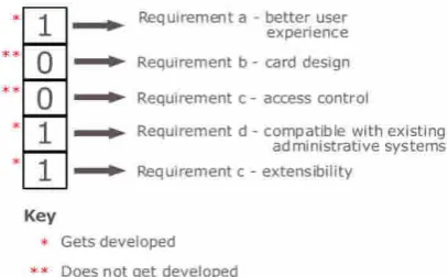
An ‘individual’ as used in this research work is a decision vector whose dimensionality is the total number of the set of requirements used, that is, the size of input. The values of the elements in this individual is either 0 or 1 signifying whether or not the corresponding the requirement is selected.
Fig. 6. Sample ‘individual’ structure, showing decision vector with elements representing requirements
4. RESULTS
4.1 The RALIC Datasets
In the research work, a method of identifying and prioritizing stakeholders (which was called StakeNet) was developed. This method builds a stakeholders' social network, using an initial set recommendations of stakeholders by other stakeholders which makes up the links in the social network. The method then prioritizes the stakeholders in the network based on these recommendations. This kind of prioritization of stakeholders is an important factor in the method developed for identifying and prioritizing requirements – StakeRare, which also makes use of social networks and collaborative filtering in building a stakeholders’ recommendations system. Similar to the method of the StakeNet, stakeholders from the StakeNet provide ratings to an initial list of requirements while suggesting other requirements to be added to the network. The StakeRare then uses the ratings and the priorities of the stakeholders from the StakeNet in prioritizing the requirements ([Lim10]). In accordance with the model used in this research, the overall significance of the stakeholders who have requested for a particular requirement has a direct impact on the total perceived value of the stakeholders’ ratings on each requirement. An aggregate of the recommendations for every stakeholder is therefore collected. This aggregate for each stakeholder is then multiplied with the stakeholder’s rating for each requirement, with the resulting value replacing the original rating value for the requirement by the stakeholder. These newly computed ratings for each requirement are then summed up to get the total value for each requirement. These values for each requirement and the corresponding costs are then loaded as part of the inputs to the algorithm for optimization.
4.2 Results from the Hybrid Metaheuristic Algorithm
The hybrid algorithm (Variable Neighbourhood Search and Tabu Search – VNSTS) requires the following as input:
1. n – An integer number, representing the number of neighbourhood structures to be created. This parameter can be used to control the number of individuals in the result set. The algorithm will have at least n individuals in its result set.
2. r – A floating point number between 0 and 1, representing the probability that the value of an element of a decision vector in each individual is 0, that is, the smaller the number r, the higher the chance that the value of an element in a decision vector will be 1, and vice versa. This parameter can be used to
control number of ‘accept’ decisions present in each generated individual.
3. d – An integer number denoting the dimensionality of each individual. This is the number of requirements that the algorithm will take. Each element of the decision vector in each individual corresponds to a decision whether or not to fulfill a requirement, that is, a one to one mapping exists between the elements and the requirements, hence, dimensionality equals number of requirements.
4. A structured list of requirements containing value and cost for each requirement.
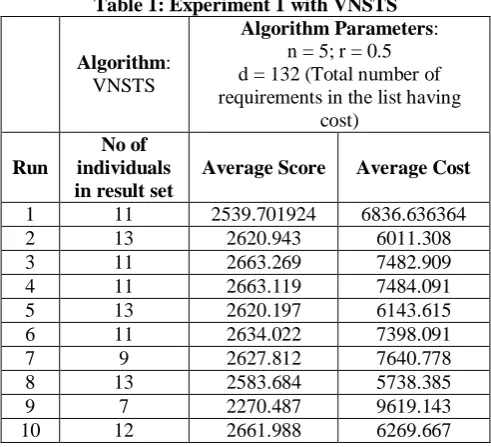
The following tables and figures show the summary of the various results gotten from multiple runs of the VNSTS algorithm, using the requirement list in Table 5 above as input, alongside other parameters set. The average of the score and cost of all the individuals is calculated for the result set in each run. Each result set contains a set of individuals, each representing decision vectors for the input requirement sets. In each of the tables, the cardinality of the result set is given under the heading ‘No of individuals in result set’. Each individual in each result set contains a different combination of decisions ‘Accept’ or ‘Decline’ for each requirement with the score and cost of only requirements with ‘Accept’ decision added together to make up the score and cost value for the particular individual. The average score and cost values of the individuals in the result set of every run is then calculated.
Table 1: Experiment 1 with VNSTS
Algorithm: VNSTS
Algorithm Parameters: n = 5; r = 0.5 d = 132 (Total number of requirements in the list having
cost)
Run
No of individuals in result set
Average Score Average Cost
1 11 2539.701924 6836.636364 2 13 2620.943 6011.308 3 11 2663.269 7482.909 4 11 2663.119 7484.091 5 13 2620.197 6143.615 6 11 2634.022 7398.091 7 9 2627.812 7640.778 8 13 2583.684 5738.385 9 7 2270.487 9619.143 10 12 2661.988 6269.667
for each run from what is obtainable in experiment 1 in Table 1 where the value of n is set to 5.
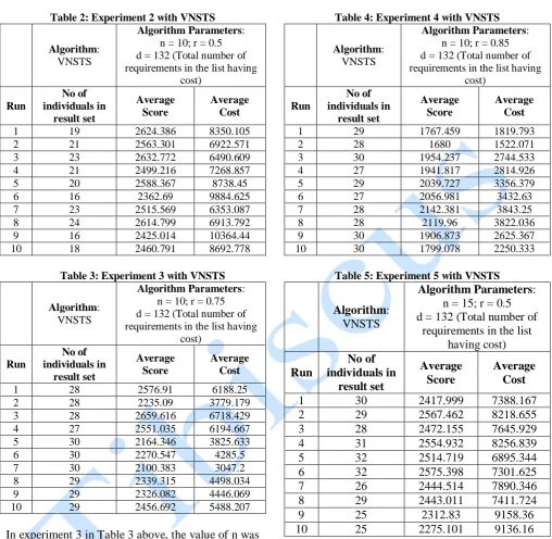
Table 2: Experiment 2 with VNSTS
Algorithm: VNSTS
Algorithm Parameters: n = 10; r = 0.5 d = 132 (Total number of requirements in the list having
cost)
Run
No of individuals in
result set
Average Score
Average Cost
1 19 2624.386 8350.105 2 21 2563.301 6922.571 3 23 2632.772 6490.609 4 21 2499.216 7268.857 5 20 2588.367 8738.45 6 16 2362.69 9884.625 7 23 2515.569 6353.087 8 24 2614.799 6913.792 9 16 2425.014 10364.44 10 18 2460.791 8692.778
Table 3: Experiment 3 with VNSTS
Algorithm: VNSTS
Algorithm Parameters: n = 10; r = 0.75 d = 132 (Total number of requirements in the list having
cost)
Run
No of individuals in
result set
Average Score
Average Cost
1 28 2576.91 6188.25
2 28 2235.09 3779.179 3 28 2659.616 6718.429 4 27 2551.035 6194.667 5 30 2164.346 3825.633
6 30 2270.547 4285.5
7 30 2100.383 3047.2
8 29 2339.315 4498.034 9 29 2326.082 4446.069 10 29 2456.692 5488.207
In experiment 3 in Table 3 above, the value of n was kept at 10 while the value of r is increased to 0.75. This led to a consequential increment in the number of individuals in the result set for each run, compared to the results in the experiment in Table 3, which has the same value for n, but a smaller r value. Also, at 0.75 value for r, the number of individuals in each result set seems to vary less often. Furthermore, the score and cost values have reduced slightly. This is because there is now a 0.75 probability that a requirement would be declined. In experiment 4 in Table 4, the value of n was also kept at 10 while the value of r is increased to 0.85. This did not bring any significant change to the range of number of individuals in each result set to what is obtained in Table 3. However, the score and cost values have decreased even more; the
probability that a requirement would be declined is now 0.85.
Table 4: Experiment 4 with VNSTS
Algorithm: VNSTS
Algorithm Parameters: n = 10; r = 0.85 d = 132 (Total number of requirements in the list having
cost)
Run
No of individuals in
result set
Average Score
Average Cost
1 29 1767.459 1819.793
2 28 1680 1522.071
3 30 1954.237 2744.533 4 27 1941.817 2814.926 5 29 2039.727 3356.379 6 27 2056.981 3432.63 7 28 2142.381 3843.25
8 28 2119.96 3822.036
9 30 1906.873 2625.367 10 30 1799.078 2250.333
Table 5: Experiment 5 with VNSTS
Algorithm: VNSTS
Algorithm Parameters: n = 15; r = 0.5 d = 132 (Total number of
requirements in the list having cost)
Run
No of individuals in
result set
Average Score
Average Cost
1 30 2417.999 7388.167
2 29 2567.462 8218.655
3 28 2472.155 7645.929
4 31 2554.932 8256.839
5 32 2514.719 6895.344
6 32 2575.398 7301.625
7 26 2444.514 7890.346
8 29 2443.011 7411.724
9 25 2312.83 9158.36
10 25 2275.101 9136.16
In experiment 5 in Table 5 above, the value of r is set back to 0.5 while the value of n is increased to 15. Comparing the results in this table with those in Table 2 which has the same value of r and a smaller value of n, it is noted that the range of numbers of individuals in the results in Table 5 is significantly larger than what is obtained in Table 2. This effect is due to the change in the value of n.
Table 6: Experiment 6 with VNSTS
Algorithm: VNSTS
Algorithm Parameters: n = 50; r = 0.85; d = 132 (Total number of requirements in the list
having cost)
Run
No of individuals in result set
Average Score Average Cost
1 130 1917.266 2647.185 2 120 1897.43 2479.75 3 125 2057.485 3424.112
4 126 1990.807 3168
5 126 1920.05 2762.476
From the results from the various experiments performed on the VNSTS algorithm, it was noticed that for the same size of requirement list and value of n, runs that have higher number of individuals in their result set have higher score averages and lower cost averages and hence, could be deemed to have better the results. It was also noticed that the number of individuals in the result set increases with the value of n and also slightly with the value of r, while the score and cost values reduce when r was increased and also when n was increased. The number of individuals in the result set also seems to converge at 0.75 value of r. Another important discovery is that higher values of n did not have any significant effects on the execution time of the algorithm.
Furthermore, the differences between the score values in each of the runs in each of the experiments performed seems to be less pronounced as the differences between the cost values, this is because the differences between the cost values in the input requirements list in Table 1 are much more pronounced than the differences between the score values. Such differences are therefore not due to the method of solution.
4.3 Results from NSGA-II Algorithm
The NSGA-II requires the following as input: 1. g – An integer, representing the number of
generations the algorithm gets to, that is, the algorithm will generate g generations. This is the major stopping condition for the algorithm. 2. p – An integer, representing the number of
individuals in each population
3. d – An integer, representing the dimensionality of each individual, that is, the number of genes each individual has. This is the number of requirements that the algorithm will take. Each element of the decision vector in each individual corresponds to a decision whether or not to fulfill a requirement, that is, a one to one mapping exists between the elements and the requirements, hence,
dimensionality equals number of requirements.
4. t – An integer number representing tournament size. This number is used when selecting parents for mating. A group of individuals of size t is selected from the population, with the fittest of them chosen as a parent.
5. ps – An integer number representing mating pool size. ps number of parents are selected into the mating pool for mating
6. mp – A floating point number representing the probability that a gene of a child individual will be not be gotten from either of its parents. 7. u – A floating point number representing the
uniformity of the amount of genes that a child gets from either parents during crossover. 8. A structured list of requirements having value
and cost for each requirement.
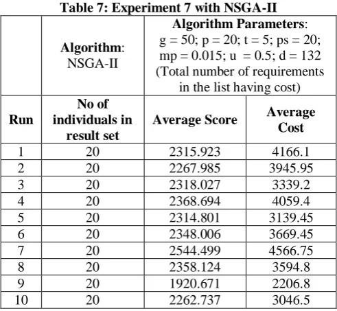
The following tables and figures show the summary of the various results from multiple experiments with the NSGA-II algorithm, using the requirement list in Table 5 above as input, alongside other parameters set, guided by recommendations from literature. As it is with the experiments in the previous section, the average of the score and cost of all the individuals is calculated for the result set in each run. Each result set contains a set of individuals, each representing decision vectors for the input requirement sets. In each of the tables, the cardinality of the result set is given under the heading ‘No of individuals in result set’. Each individual in each result set contains a different combination of decisions ‘Accept’ or ‘Decline’ for each requirement with the score and cost of only requirements with ‘Accept’ decision added together to make up the score and cost value for the particular individual. The average score and cost values of the individuals in the result set of every run is then calculated.
Table 7: Experiment 7 with NSGA-II
Algorithm: NSGA-II
Algorithm Parameters: g = 50; p = 20; t = 5; ps = 20; mp = 0.015; u = 0.5; d = 132 (Total number of requirements
in the list having cost)
Run
No of individuals in
result set
Average Score Average Cost
1 20 2315.923 4166.1
2 20 2267.985 3945.95
3 20 2318.027 3339.2
4 20 2368.694 4059.4
5 20 2314.801 3139.45 6 20 2348.006 3669.45 7 20 2544.499 4566.75
8 20 2358.124 3594.8
9 20 1920.671 2206.8
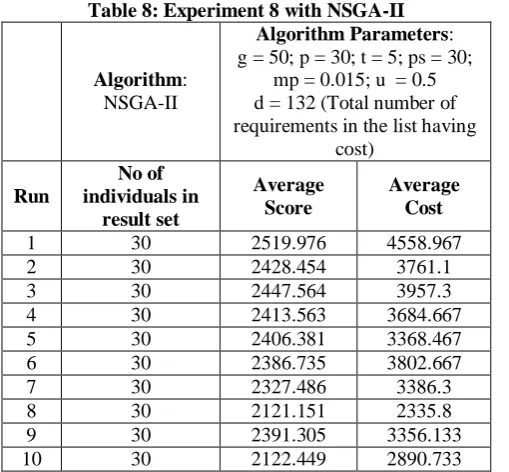
Table 8: Experiment 8 with NSGA-II
Algorithm: NSGA-II
Algorithm Parameters: g = 50; p = 30; t = 5; ps = 30;
mp = 0.015; u = 0.5 d = 132 (Total number of requirements in the list having
cost)
Run
No of individuals in
result set
Average Score
Average Cost
1 30 2519.976 4558.967
2 30 2428.454 3761.1
3 30 2447.564 3957.3
4 30 2413.563 3684.667 5 30 2406.381 3368.467 6 30 2386.735 3802.667
7 30 2327.486 3386.3
8 30 2121.151 2335.8
9 30 2391.305 3356.133 10 30 2122.449 2890.733
In experiment 8 in Table 8 above, comparing with experiment 7 in Table 7, the population size p and the size of mating pool are both set to 30 in Table 8, increased from the value of 20 set in Table 7. Results in both tables show that the number of individuals in each result set is the same as the size of the population. Results in Table 8 (with an increased population size) show a slight increase in the average score and cost values of run.
In experiment 9 in Table 9, the population size and the size of mating pool were increased further to 40. This led to an increased number of individuals in the result set, and a slight, almost negligible increase in the score averages of each run.
Experiments with the NSGA-II algorithm show that the score and cost values increase slightly with an increase in population size p, however, time of
execution also increases significantly with an increase in population size p. It is therefore difficult for a decision maker to control the level of score and cost values and target a desirable range.
Table 9: Experiment 9 with NSGA-II
Algorithm: NSGA-II
Algorithm Parameters: g = 50; p = 40; t = 5; ps = 40;
mp = 0.015; u = 0.5 d = 132 (Total number of requirements in the list having
cost)
Run
No of individuals in
result set
Average Score
Average Cost
1 40 2382.491 3424.35
2 40 2321.328 3367
3 40 2449.157 3450.45 4 40 2402.444 3216.475 5 40 2517.614 3820.45 6 40 2217.521 2580.175 7 40 2330.445 3248.075 8 40 2413.783 3641.325 9 40 2445.492 3636.55 10 40 2354.887 3727.85
The table below gives a comparison of result sets having about the same number of individuals selected from experiments with VNSTS and NSGA-II algorithms. A score-cost ratio is calculated for each. The table show some results from the NSGA-II algorithm having better score-cost ratio.
The following table gives a summary of the findings from the experiments conducted with VNSTS and NSGA-II:
Table 10: Comparison of results from VNSTS and NSGA-II
NSGA-II VNSTS
No of
Individuals Score Cost
Score/Cost Ratio
No of
Individuals Score Cost
Score/Cost Ratio 30 2519.976 4558.967 0.552752 30 2164.346 3825.633 0.565748 30 2428.454 3761.1 0.645677 30 2270.547 4285.5 0.529821 30 2447.564 3957.3 0.618493 30 2100.383 3047.2 0.689283 30 2413.563 3684.667 0.655029 30 1954.237 2744.533 0.712047 30 2406.381 3368.467 0.714385 30 1906.873 2625.367 0.726326 30 2386.735 3802.667 0.627648 30 1799.078 2250.333 0.799472 30 2327.486 3386.3 0.687324 30 2417.999 7388.167 0.32728 30 2121.151 2335.8 0.908105 29 2339.315 4498.034 0.520075 30 2391.305 3356.133 0.712518 29 2326.082 4446.069 0.523177 30 2122.449 2890.733 0.734225 29 2456.692 5488.207 0.447631
5. SUMMARY
This research work described how a hybrid of Variable Neighbourhood Search and Tabu Search could be applied to the Next Release Problem in Software Engineering. The Next Release Problem (NRP) is a problem arising from the need for a software engineer to decide on what requirements to develop as features in the next release of the software being developed from a long list of competing requirements, having costs and perceived values, all of which cannot be developed given a limited resources. The software engineer is interested in maximizing the total value gotten from the selected requirements while minimizing the cost of developing them. The choice of the method of solution is based on the work of Garcia-Torres et al. ([G+04]) who applied a hybrid of Variable Neighbourhood Search and Tabu Search to solving the Feature Subset Selection problem which the NRP is a type of ([B+06, ZHM07]). The model used in this project is a cost-value model for requirements ([ZHM07, D+11]), where only two objectives are considered with cost formulated as an objective. The real world Replacement Access, Library and ID Card project (RALIC) datasets ([Lim10], [LF12]) were used in performing experiments with the hybrid algorithm. The state-of-the-art algorithm NSGA-II was also implemented, with experiments carried out using the same data. Experiments showed that for result sets having the same number of individuals from either algorithms, some of the results from NSGA-II were slightly better. However, trade-offs such as easier and cheaper parameter tuning, larger solution set were discovered with the NSGA-II.
6. CONCLUSION
Experiments have shown that the VNSTS algorithm gives results with a relatively large and dynamic number of individuals with a predictable range, such that a decision maker can predetermine the range of the number of choices he would prefer by manipulating the algorithm parameters. A decision maker can also predetermine the range of score and cost values for which a Pareto optimal set is needed by manipulating the algorithm parameters.
Furthermore, from the results gotten from the experiments performed, it can be deduced that the VNSTS is a ‘good enough’ algorithm for application on the NRP, especially when the decision maker has a target cost value and he wishes to tune the algorithm parameters easily and cheaply (in terms of computational power), and also when the decision maker wants a very much wide set of options from which to select from.
Moreover, from the results of the experiments conducted, the VNSTS algorithm shows a good prospect, arriving at ‘good enough’ solutions, this means that it can be applied to solving other optimization problems, in and out of software engineering
7. RECOMMENDATION AND FUTURE
WORK
Informed by the prospects demonstrated by the VNSTS algorithm, further application of the algorithm on other search based software engineering areas is recommended. A more problem specific approach could be researched for each application to increase the chance of getting even better results. This research considered two objectives in the NRP, further application of the VNSTS could be done on the NRP, using a single objective or many (more than two) objectives with risk uncertainty.
Furthermore, since the VNSTS algorithm is an optimization algorithm, and given the success in its application on the FSS problem in literature and on NRP in this project, application of the VNSTS on other optimization problems is therefore a good way to proceed.
REFERENCES
[AAG10] F. Asadi, G. Antoniol, Y. Gueheneuc
- Concept locations with genetic algorithms: A comparison of four distributed architectures. In Proceedings of 2nd International Symposium on Search based Software Engineering (SSBSE 2010), Benevento, Italy, 2010. IEEE Computer Society Press.
[AGS16] S. Agarwal, S. Gupta, N. Sabharwal - Automatic Test Data Generation-Achieving Optimality Using Ant-Behaviour. International Journal of Information and Education Technology, Vol. 6, No. 2, February 2016.
[Bro15] J. Brownlee - Clever Algorithms: Nature-Inspired Programming Recipes. 2015.
http://www.cleveralgorithms.com/natur e-inspired/stochastic/tabu_search.html
[accessed 16/6/2016].
problem. Information and Software Technology 43 pgs. 883 – 890, 2001. [BSA06] S. Bouktif, H. Sahraoui, G. Antoniol -
Simulated Annealing for Improving Software Quality Prediction. In Proceedings of the 8th annual Conference on Genetic and Evolutionary Computation (GECCO ’06), pages 1893–1900, Seattle, Washington, USA. ACM, 2006.
[B+06] P. Baker, M. Harman, K. Steinhofel,
A. Skaliotis - Search Based
Approaches to Component Selection and Prioritization for the Next Release Problem. 22nd IEEE International Conference on Software Maintenance (ICSM '06), 2006.
[CA07] B. H. C. Cheng, J. M. Atlee - Research directions in requirements engineering. Proceedings of international conference on software engineering, ISCE 2007. Workshop on the future of software engineering (FOSE 2007). Minneapolis, pp 285– 303, 2007.
[DG97] M. Dorigo, M. Gambardella - Ant Colony System: A Cooperative Learning Approach to the Traveling Salesman Problem. IEEE Transactions on Evolutionary Computation. Vol. 1 Issue 1, 1997.
[D+02] K. Deb, A. Pratap, S. Agarwal, T. Meyarivan - A Fast and Elitist Multiobjective Genetic Algorithm: NSGA-II. IEEE Transactions on Evolutionary Computation. Vol 6, Issue 2. Pages 182-197, 2002.
[D+11] J. J. Durillo, Y. Zhang, E. Alba, M. Harman, A. J. Nebro - A Study of the Bi-Objective Next Release Problem. Empirical Software Engineering. February 2011, Volume 16, Issue 1, pp 29-60.
[D+15] J. del Sagrado, I. M. del Aguila, F. J. Orellana - Multi-objective ant colony optimization for requirements selection. Empirical Software Engineering. June 2015, Volume 20, Issue 3, pp 577-610, 2015.
[Gen03] M. Gendreau - An introduction to tabu search. Volume 57 of the series if the International Series in Operations Research & Management Science pp 37-54, 2003.
[Glo89] F. Glover - Tabu Search-Part I. Operations Research Society of America Journal on Computing Vol. 1, No. 3, Summer 1989.
[God97] P. Godefroid - Model Checking for Programming Languages using Verisoft. In Proceedings of the 24th ACM SIGPLAN-SIGACT symposium on Principles of Programming Languages, pages 174–186, Paris, France. ACM, 1997.
[GHA09] S. Gueorguiev, M. Harman, G. Antoniol - Software Project Planning for Robustness and Completion Time in the Presence of Uncertainty using Multi Objective Search Based Software Engineering. GECCO 09. Proceedings of the 11th annual conference on genetic and evolutionary computation. Pages 1673-1680, 2009.
[G+04] M. Garcia-Torres, F. Garcia-Lopez, B. Melian-Batista, J. A. Moreno-Perez, J. M. Moreno-Vega - Solving Feature Subset Selection Problem by a Hybrid Metaheuristic, 2004.
[Har10] M. Harman - Why the Virtual Nature of Software Makes it Ideal for Search Based Optimization. Fundamental Approaches to Software Engineering. Volume 6013 of the series Lecture Notes in Computer Science, pp 1-12, 2010.
[Hol75] J. H. Holland - Adaption in Natural and Artificial Systems. MIT Press, Ann Arbor, 1975.
[HC04] M. Harman, J. Clark - Metrics are fitness functions too. 10th International Software Metrics Symposium (METRICS 2004), pages 58–69, Los Alamitos, California, USA, September 2004. IEEE Computer Society Press. [HJ01] M. Harman, B. F. Jones -
Information and Software Technology 43. Pgs. 883 – 839, 2001.
[HM01] P. Hansen, N. Mladenovic - Variable neighborhood search: Principles and applications. European Journal of Operational Research. Volume 130, Issue 3, 1 May 2001, pp 449–467. [HM10] M. Harman, A. Mansouri - Search
Based Software Engineering: Introduction to the Special Issue of the IEEE Transactions on Software Engineering. IEEE Transactions on Software Engineering, Vol. 36, No. 6, November/December 2010.
[HT07] M. Harman, L. Tratt - Pareto Optimal Search Based Refactoring at the Design Level. Proceedings of the 9th annual conference on genetic and evolutionary computation. GECCO 07 pp. 1106-1113, 2007.
[HKF08] P. He, L. Kang, M. Fu - Formality Based Genetic Programming. In Proceedings of the IEEE Congress on Evolutionary Computation (CEC ’08) (IEEE World Congress on Computational Intelligence), pages 4080–4087, Hong Kong, China. IEEE Press, 2008.
[HMZ09] M. Harman, S. A. Mansouri, Y. Zhang - Search Based Software Engineering: A Comprehensive Analysis and Review of Trends Techniques and Applications. Technical Report TR-09-03, Department of Computer Science, King’s College London, April 2009.
[H+12] M. Harman, P. McMinn, J. Teixeira de Souza, S. Yoo - Search Based Software Engineering: Techniques, Taxonomy, Tutorial. Empirical Software Engineering and Verification, Volume 7007 of the series Lecture Notes in Computer Science pp 1-59, 2012.
[Joh07] C. Johnson - Genetic Programming with Fitness based on Model Checking. In Proceedings of the 10th European Conference on Genetic Programming, volume 4445 of LNCS, pages 114–124, Valencia, Spain. Springer, 2007.
[KP08] G. Katz, D. Peled - Genetic Programming and Model Checking: Synthesizing New Mutual Exclusion Algorithms. In Proceedings of the 6th International Symposium on Automated Technology for Verification and Analysis (ATVA ’08), volume 5311 of LNCS, pages 33–47, Seoul, Korea. Springer, 2008.
[K+08] P. Kapur, A. Ngo-The, G. Ruhe, A. Smith - Optimized staffing for product releases and its application at Chartwell Technology. J. Softw. Maint. Evol.: Res. Pract., 20: 365–386. doi: 10.1002/smr.379, 2008.
[Lim10] S. L. Lim - Social Networks and Collaborative Filtering in Large-Scale Requirements Elicitation. PhD Thesis. School of Computer Science and Engineering, University of New South Wales, Sydney, Australia, 2010.
[LF12] S. L. Lim, A. Finkelstein - StakeRare: Using Social Networks and Collaborative Filtering for Large-Scale Requirements Elicitation. IEEE Transactions on Software Engineering. Issue 3 Volume 38, pages 707 – 735, 2012.
[Min04] P. McMinn - Search-based Software Test Data Generation: A Survey. Software Testing, Verification and Reliability, 14(2), 105–156, 2004. [Min11] P. McMinn - Search-based testing:
Past, present and future. In Proceedings of the 3rd International Workshop on Search-Based Software Testing (SBST 2011), Berlin, Germany, 2011, To Appear. IEEE, 2011.
[MB06] P. K. Mahanti, S. Banerjee - Automated Testing in Software Engineering: using Ant Colony and Self-Regulated Swarms. In Proceedings of the 17th IASTED international conference on Modelling and simulation (MS ’06), pages 443–448, Montreal, Canada. ACTA Press, 2006. [MS76] W. Miller, D. Spooner - Automatic
[Nic12] B. Nicholas - The relevance of efficiency to different theories of society. Economics of the Welfare State (5th ed.). Oxford University Press. p. 46. ISBN 978-0-19-929781-8, 2012. [Rai09] O. Raiha - A Survey on Search Based
Software Design. Technical Report D-2009-1, Dept. of Computer Sciences, University of Tampere, 2009.
[RPV03] W. N. Robinson, S. D. Pawlowski, V. Volkov - Requirements Interaction Management. ACM Computing Surveys (CSUR). Volume 25 Issue 2, June 2003. Pages 132-190. ACM New York, NY, USA.
[SA13] A. S. Sayyad, H. Ammar - Pareto-Optimal Search-Based Software Engineering (POSBSE): A Literature Survey. Realizing Artificial Intelligence Synergies in Software Engineering (RAISE), 2013 2nd International Workshop. 00. 21-27, 2013.
[SX93] M. Schoenauer, S. Xanthakis - Constrained GA Optimization. In Proceedings of the 5th International Conference on Genetic Algorithms (ICGA ’93), pages 573–580, San Mateo, CA, USA. Morgan Kauffmann, 1993.
[V+05] J. M. Van den Akker, S.
Brinkkemper, G. Diepen, J.
Versendaal - Determination of the next release of a software product: an approach using integer linear programming. In: Proceeding of the 11th International Workshop on Requirements Engineering: Foundation for Software Quality (REFSQ 2005), pp. 119–124, 2005.
[ZH10] Y. Zhang, M. Harman - Search Based Optimization of Requirements Interaction Management. Search Based Software Engineering (SSBSE), 2010 Second International Symposium. 7-9 Sept. 2010. pp 47-56, 2010.
[ZHL13] Y. Zhang, M. Harman, S. L. Lim - Empirical Evaluation of Search Based Requirements Interaction Management. Information and Software Technology. January 2013, Vol.55(1): 126-152. [ZHM07] Y. Zhang, M. Harman, S. A.
![Fig. 1. Example of SBSE in requirements selection and regression testing ([H+12])](https://thumb-us.123doks.com/thumbv2/123dok_us/8959531.1868899/2.595.310.540.359.612/fig-example-sbse-requirements-selection-regression-testing-h.webp)
![Fig. 3. Random search may not find optimal solutions ([Min11])](https://thumb-us.123doks.com/thumbv2/123dok_us/8959531.1868899/3.595.324.543.385.544/fig-random-search-optimal-solutions-min.webp)
![Fig. 4. Hill climbing algorithm ([Min11])](https://thumb-us.123doks.com/thumbv2/123dok_us/8959531.1868899/4.595.46.278.471.616/fig-hill-climbing-algorithm-min.webp)
![Fig. 5. Global search Genetic Algorithms, considering various points in the search space ([Min11])](https://thumb-us.123doks.com/thumbv2/123dok_us/8959531.1868899/5.595.96.252.117.212/global-search-genetic-algorithms-considering-various-points-search.webp)