APPLICATION OF MARKOV PROCESSES
TO THE MACHINE DELAYS ANALYSIS
M. Saidi-Mehrabad
Department of Industrial Engineering, Iran University of Science and Technology
Narmak, 16844, Tehran, Iran, [email protected]
(Received: June 7, 2000 – Accepted in Revised Form: October 23, 2001)
Abstract Production and non-productive equipment and personnel delays are a critical element of any production system. The frequency and length of delays impact heavily on the production and economic efficiency of these systems. Machining processes in wood industry are particularly vulnerable to productive and non-productive delays. Whereas, traditional manufacturing industries usually operate on homogeneous raw material, in a restricted environment with closely controlled processing guidelines. The logging industry must continually deal with a raw material that comes in many different shapes, sizes and performs in an environment that is different from site to site. Furthermore, loggers; rarely have the opportunity to follow a predetermined production sequence, as men and machines must maneuver as conditions dictate. As a result machining systems can experience a broad range of delays that vary widely in frequency and length. The purpose of this study was to apply Markov process models to the analysis of delay times in machining processes. Such an approach will permit the random components of machining process to be integrated into a flexible mathematical model, using theoretical probability distributions, and providing analytic solutions to proportions of productive delay time.
Key Words Delays Analysis, Markov Process
ﻩﺪﻴﻜﭼ
ﺪﻨﺘﺴﻫ ﻱﺪﻴﻟﻮﺗ ﻢﺘﺴﻴﺳ ﺮﻫ ﻲﻧﺍﺮﺤﺑ ﻞﻣﺍﻮﻋ ﻲﻠﻨﺳﺮﭘ ﺕﺍﺮﻴﺧﺎﺗ ﻭ ﻱﺪﻴﻟﻮﺗﺮﻴﻏ ﻭ ﻱﺪﻴﻟﻮﺗ ﺕﺍﺰﻴﻬﺠﺗ .
ﻭ ﻲﻟﺍﻮﺗ
ﻣ ﺮﺑ ﺮﻴﺧﺎﺗ ﻝﻮﻃ ﻩﺮﻬﺑ ﻥﺍﺰﻴ
ﻲﻣ ﺮﻴﺛﺎﺗ ﺎﻬﻤﺘﺴﻴﺳ ﻦﻳﺍ ﺪﻴﻟﻮﺗ ﻭ ﻱﺭﻭ ﺪﻧﺭﺍﺬﮔ
. ﺯﺍ ﺏﻮﭼ ﻊﻳﺎﻨﺻ ﺭﺩ ﻱﺭﺎﻜﻨﻴﺷﺎﻣ ﺪﻨﻳﺍﺮﻓ
ﺭﺩ ﻷﻮﻤﻌﻣ ﻲﺘﻨﺳ ﻱﺪﻴﻟﻮﺗ ﻊﻳﺎﻨﺻ ﻪﻜﻳﺭﻮﻄﺑ ؛ﺖﺳﺍ ﺮﻳﺬﭘ ﺮﻴﺛﺎﺗ ﻱﺪﻴﻟﻮﺗ ﺮﻴﻏ ﻭ ﻱﺪﻴﻟﻮﺗ ﻢﺘﺴﻴﺳ ﺯﺍ ﻲﺷﺎﻧ ﺕﺍﺮﻴﺧﺎﺗ ﻲﻣ ﺭﺎﻛ ﺖﺧﺍﻮﻨﻜﻳ ﺩﺍﻮﻣ ﻱﻭﺭ ،ﻩﺪﺷ ﻝﺮﺘﻨﻛ ﻲﻠﻤﻌﻟﺍﺭﻮﺘﺳﺩ ﺎﺑ ﻭ ﺩﻭﺪﺤﻣ ﻲﻄﻴﺤﻣ ﺪﻨﻨﻛ
. ﺎﻨﺻ ﻡﻮﻤﻋ ﺩﺍﻮﻣ ﺎﺑ ،ﻱﺮﺑ ﺏﻮﭼ ﻊﻳ
ﻩﺯﺍﺪﻧﺍ ﻭ ﻝﺎﻜﺷﺍ ﻱﺍﺭﺍﺩ ﻡﺎﺧ
ﺪﻧﺭﺍﺩ ﺭﺎﻛﻭﺮﺳ ﻉﻮﻨﺘﻣ ﻱﺭﺎﻛ ﻂﻴﺤﻣ ﻭ ﺕﻭﺎﻔﺘﻣ ﻱﺎﻫ .
ﻱﺍﺮﺑ ﻲﻤﻛ ﺲﻧﺎﺷ ﻷﻮﻤﻌﻣ ﻊﻳﺎﻨﺻ ﻦﻳﺍ
ﺪﻧﺭﺍﺩ ﺪﻴﻟﻮﺗ ﻪﺑ ﻁﻮﺑﺮﻣ ﻲﻟﺎﻤﺘﺣﺍ ﻱﺎﻬﺘﻴﻌﻗﻮﻣ ﺎﺑ ﻦﻴﺷﺎﻣ ﻭ ﺮﮔﺭﺎﻛ ،ﻩﺪﺷ ﻦﻴﻴﻌﺗ ﻞﺒﻗ ﺯﺍ ﺕﺎﻴﻠﻤﻋ ﻑﺩﺍﺮﺗ .
ﻱﺎﻬﻤﺘﺴﻴﺳ
ﺗ ﻱﺩﺎﻳﺯ ﺩﺍﺪﻌﺗ ﻞﺑﺎﻘﻣ ﺭﺩ ،ﻪﺠﻴﺘﻧ ﺭﺩ ،ﻲﻨﻴﺷﺎﻣ
ﺪﻧﺭﺍﺩ ﺭﺍﺮﻗ ﺮﻴﻐﺘﻣ ﻲﻟﺍﻮﺗ ﻭ ﻲﻧﺎﻣﺯ ﻝﻮﻃ ﻱﺍﺭﺍﺩ ﺕﺍﺮﻴﺧﺎ .
ﻦﻳﺍ
ﻑﺪﻫ
ﻭ
ﻩﺩﻮﺑ
ﻱﺭﺎﻜﻨﻴﺷﺎﻣ
ﺪﻨﻳﺍﺮﻓ
ﺭﺩ
ﺮﻴﺧﺎﺗ
ﻥﺎﻣﺯ
ﻞﻴﻠﺤﺗ
ﻭ
ﻪﻳﺰﺠﺗ
ﻱﺍﺮﺑ
ﻮﻛﺭﺎﻣ
ﻩﺮﻴﺠﻧﺯ
ﻱﺎﻬﻟﺪﻣ
ﻱﺮﻴﮔﺭﺎﻜﺑ
،ﻖﻴﻘﺤﺗ
ﻩﺍﺭ
ﻭ
ﻲﻟﺎﻤﺘﺣﺍ
ﻊﻳﺯﻮﺗ
ﻱﺎﻬﻳﺭﻮﺌﺗ
ﺯﺍ
ﻩﺩﺎﻔﺘﺳﺍ
ﺎﺑ
ﻱﺭﺎﻜﻨﻴﺷﺎﻣ
ﺪﻨﻳﺍﺮﻓ
ﻲﻗﺎﻔﺗﺍ
ﻱﺍﺮﺟﺍ
ﻱﺯﺎﺳ
ﻪﭼﺭﺎﭘ
ﻚﻳ
ﻥﺎﻜﻣﺍ
ﺤﺗ
ﻭ
ﻪﻳﺰﺠﺗ
ﻞﺣ
ﻲﻣ
ﺩﻮﺟﻮﺑ
ﻲﺿﺎﻳﺭ
ﻝﺪﻣ
ﻚﻳ
ﻂﺳﻮﺗ
ﺍﺭ
ﺪﻴﻟﻮﺗ
ﺮﻴﺧﺎﺗ
ﻥﺎﻣﺯ
ﺎﺑ
ﺐﺳﺎﻨﺘﻣ
ﻞﻴﻠ
ﺩﺭﻭﺁ
.INTRODUCTION
The uncontrollable interaction offers a unique and complex problem for effectively analyzing machine delays. For any new technique to become generally accepted, it must be able to handle the analysis of uncontrollable interactions. To become competitive with simulation modeling, a new technique must not only handle the uncontrollable interaction, but also improve upon the performance of simulation in these situations. Productive and non-productive equipment
and personnel delays are a critical element of any production system. The frequency and length of delays impact heavily on the production and economic efficiency of these systems.
models, the Markov model improves upon this by providing an analytic solution. The Markov model also avoids the problems of correlated output data from simulations by explicitly recognizing that any possible future state is dependent only on the current state of the system and is conditionally independent of the past history of the system. The methodology for building a Markov model requires dealing with only two probability distributions, the Erlang and mixed Erlang, for modeling time based activities (such as cycle times) of the interacting machines. These probability distributions in turn, provide the necessary data for developing a system of algebraic equations for solving the Markov process model.
BACKGROUND
With well-developed techniques for analyzing productivity in traditional industries, we see a great deal of this methodology extrapolated to the non-traditional timber-harvesting environment. The constancy of traditional industrial productivity has led to standardization in a very deterministic fashion (i.e., usually via regression estimates). Managers are most concerned with developing normal performance ratings that provide benchmarks for evaluating employee performance. Traditional industrial productivity is assumed to approximate a normal distribution [1]. Normally distributed production times are taken as indicative of consistent work habits and normal work pacing, Steffy and Darby [2]. Cite non-symmetric production distributions as evidence of some abnormality. Positively skewed distributions are deemed to be indicative of restricted work output, due possibly to machine cycle time restrictions or other dependent operations. Alternatively, negatively skewed productivity distributions may indicate a worker is motivated to work slowly, but sets a limit on maximum cycle time. Applying general statements of this type to timber harvesting would be improper, since the variation in operating conditions will inevitably cause departure from symmetry in performance distributions. Various methods have been utilized to study machine cycle time delays, including: case studies, regression analysis, and simulation. Case studies generally focus upon developing simple summary statistics from observations on a system operating in a restricted setting [3]. There is generally no attempt to build a model to analyze the system and
test possible modifications in system components.
METHODS
The purpose of this study was to apply Markov process models to the analysis of delay times in cable logging systems. Such an approach will permit the random components of the cable logging production systems to be integrated into a flexible mathematical model, using theoretical probability distributions, and providing analytic solutions to proportions of productive and delay time.
CONTINUOUS PARAMETER MARKOV THEORY
Markov process theory provides a powerful mechanism for investigating the steady-state performance of production systems. The underlying construct of all Markov processes is that the probability a system will be in a given state at time t n+1 may be determined from the
knowledge of its state at tn and is conditionally
independent of the history of the system before tn.
For this study, the state of the system is assumed to be discrete, so that it can be described in terms of specific stages or phases of production or delay. Because timber harvesting systems are configured with finite numbers of machine and personnel, operating on finite numbers of trees or stems, discrete state processes will generally be used in modeling such systems.
Continuous parameter Markov models permit an analysis of the system at any time t within any of the stages of the system, providing a more realistic analysis of logging operations where a c t i vi t i e s a n d p r o d u c t i o n l e vel c h a n ge continuously. Using a discrete parameter Markov process would restrict the analysis to fixed points in time and would not adequately describe the probabilistic behavior of the system for decision-making purposes.
steady-state behavior, the system is assumed to have
been in operation for a sufficiently long period
of time, so that any effect of these initial
conditions is largely irrelevant. Second is the
matrix of transition probabilities, p (t). Each
element of p (t), p
ij(t), represents the
probability of moving from state i to state j,
over an interval of time of length t. Of crucial
importance in continuous parameter Markov
process theory is the requirement that the
process spend a negative exponentially
distributed amount of time in state i, before
making a transition into a different state j [4].
The implication is that the time the process
spends in state i is dependent only on the state
being visited. Otherwise, information about
past or future states and the time the process
had been in the current state would be relevant
to the prediction of the next state, which
violates the Markov property.
The forgetfulness property of the exponential
and the specific type of dependence is what
guarantees that the process is Markovian.
STATISTICAL MODELS FOR DATA ANALYSIS
As stated before the major objective of this study is to determine steady-state proportions of productive and delay time for cable logging systems. A secondary objective is to illustrate how the Markov models can be formulated using basic probability and statistical tools those are relatively easy to conceptualize and use.
In an effort to maintain a high degree of utility, yet be useful and easy to understand, a single class of probability distributions is used for this analysis: Erlang distributions. Erlang distributions are very useful because they represent a large, two-parameter family of distributions permitting only nonnegative values [5]. The distributions range all the way from the “pure random” exponential type to the completely regular, constant service-time situation [6]. Although, the Erlang family will not fit all possible production/delay time distributions, they will fit many of those encountered practice. One of the recurring problems with simulation
has been the difficulty in understanding, using and interpreting the models. By sacrificing some detail (e.g., not taking the simulation approach in modeling finer and finer elements of systems with a multitude of potential statistical distributions), the Markov approach, with Erlang distributions, can be a powerful tool that provides readily accessible solutions to difficult problems. For these reasons, this study has focused on the use of Erlang distributions for model development.
The key to Erlang models is that they will permit a degree of flexibility in modeling time-based random variables (e.g., cycle times); yet maintain the integrity of the Markov model. Mathematically, the Erlang density function can be expressed as:
f(t) = [α(αt) k-1 exp(-αt)]/(k-1) (1)
where k is a positive integer and α, t>0. Parameter k and α are referred to as shape and scale parameters, respectively. The expected value of the Erlang distribution is:
E(t) = k/α (2)
and the variance is:
Var (t) = k/α2 (3)
For Markov process applications, the key here is that Erlang distributions are a sum of k independent, identically distributed exponential random variables. Each independent, identically distributed exponential represents a stage in the activity of a system component, which can be represented conceptually by a holding device with k-stages. Then, in general, for each of the k-stages, the time spent in the j-th stage is exponentially distributed as follows:
f (t) = αexp(-αt) (4)
where, α, t>0. This construction provides several requisite properties:
variable, with scale parameter α. Although the time it takes to traverse the holding device is not exponential, the combination of k-exponential stages can be considered the statistical equivalent for the purposes of the Markov model.
2. By permitting only 1 entity in the holding device at a time guarantees that the sequence of times between consecutive departures is one of independent random variables.
3. The time unit an entity departs the holding device depends only on what cell it is in, because of the forgetfulness property of the exponential distribution.
4. The concept of stages allows one to describe the movements of an entity in discrete terms.
SOLUTIONS OF THE MARKOV PROCESS MODEL
It can be shown that a steady-state solution to the Markov process model can be determined from the following system of algebraic equations [7].
πΩ = 0 (5)
where π is a vector of steady-state probabilities and
Ω is referred to as the rate matrix or generator of the Markov process.
The elements of the rate matrix, P’ ij(t)’s, are
the derivatives of the P ij(t) evaluated at t=0.
Knowing the P’ij(t)’s is equivalent to knowing Pij(t)
for every i, j, and t>0. The P’ij(t)’s are known as
transition or instantaneous rates and depict the flow of probability between states of the process. For practical applications, the P’ij(t)’s are what the
analyst seeks and in the context of this study are always the scale parameter of the Erlang distribution for the activity in question.
Rate Matrices
The rows of the rate matrix Ωare termed current states of the process, while the columns are termed future states [8]. These states are developed from the individual Erlang statistical models used in describing the time-based activities of a machine or person, where each stage of the Erlang model represents a state. The entries within the cells of the rate matrix, indexed by current and future states, represent the rate of change of probability
between different states of the system [9].
Placement of rates in the cells of the rate matrix is zero. For example, an entity with a simple n-stage Erlang model can make transitions of the form; stage (n-2) to (n-1), but the instantaneous rate of transitions such as (n-3) to (n-1) is zero. This applies equally to simultaneous transition by two components of the process. This does not mean that such changes cannot occur; only that there rate of change of probability is zero.
It is also assumed that once an entity exits the n-th stage of its Erlang model, it immediately reenters stage one of its Erlang model or enters a different Erlang model denoting a different activity. When constructing a rate matrix the following criteria must be adhered to: 1. All off-diagonal terms are positive or zero, and
since they are not probabilities but rates of change of probability, they can be greater or less than 1. 2. The diagonal terms are all negative.
3. The diagonal terms are the negative of the sum of the positive terms on the same row, so that row sums are zero.
Two very important theoretical results provide for a unique probability solution for the type of Markov model applied here: finite state space and irreducibility. Because timber-harvesting systems are configured with finite numbers of men and machines, obtaining finite state spaces does not pose a problem. Irreducibility is achieved when a positive probability exists of eventually entering any state j from any state i. In practice this condition is not difficult to meet and will be evident from the final structure of the rate matrix. With an irreducible Markov process the steady-state probabilities exist and always have the same value, irrespective of the initial probability distribution of the process. Further, with irreducibility and finite state space it is guaranteed that there exists exactly one solution for the steady-state probabilities. The steady-state probabilities are obtained by using matrix methods for solving the system of algebraic equations presented in Equation 5.
CASE STUDY
cycle time was considered representative of times over a range of conditions. As such, cycle time was used as the performance variable of interest in the analysis.
Productive Cycle Time Analysis
The meandelay free cycle time from the field data was 3.3 minutes with a standard deviation of 1.03 minutes, for the 545 cycles. Since Erlang distributions are a special case of gamma distributions, the first step in distribution fitting was to determine the maximum likelihood estimates of the shape and scale parameters. Since the shape parameter of a gamma is a real number and the Erlang shape parameter is integer, it was necessary to choose the best fitting Erlang from the next highest and next lowest integer based on the maximum likelihood fit of the gamma shape parameter. The distribution fitting analysis yielded a delay-free cycle time distribution with k = 10 and α = 2.932.
Delay Time Distributions
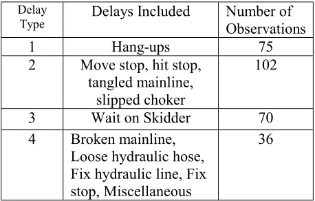
Eleven different delayswere identified in the course of the field studies, including: hang-ups, carriage delays (move stop and hit stop), mainline/choker delays (tangled, mainline, wait on skidder, slipped choker), and nonproductive carriage/line delays (broken mainline, loose hydraulic hose, fix hydraulic lines, fix stop, miscellaneous). Because of lack of data in several delay type categories, it was necessary to combine similar delays into more broadly defined groups. As a result, four groupings of delays were recognized and each group fit to an Erlang distribution (Table 1).
The summary statistics, from the field observations for each delay type are as shown in Table 2. Data in each delay grouping were fit to Erlang distributions using the same procedure outlined for delay-free cycle time. The resulting fits and their respective shape and scale parameters are summarized in Table 3.
With the fitted Erlang distributions it is now possible to describe productive and delay time within the Markov process context, by utilizing the concept of k-stage for each Erlang, where each stage is an independent and identically distributed exponential random variable with scale parameter
α. For example, productive time be conceptualized as 10 discrete stages, each requiring a random residence time equal to an exponential random variable with scale parameter α = 2.891.
Developing the Rate Matrix For Case Study
Thefirst consideration is defining the current and future state of the rate matrix. For the productive time component of the system there are 10 current and 10 future state that the system can occupy, as defined by the k = 10 Erlang model. For descriptive purposes, the state descriptor of the productive component will be defined as {pi}, where i = 1, 2, 3, …, 10, denoting the
Erlang stages of the productive cycle time model. There are four different delay types that the system can encounter, with a total of seven exponential stages. If only one delay occurred on any given cycle a 17x 17 rate matrix could TABLE 1. Four Types of Delays.
Delay
Type Delays Included Number of Observations
1 Hang-ups 75 2 Move stop, hit stop,
tangled mainline, slipped choker
102
3 Wait on Skidder 70
4 Broken mainline, Loose hydraulic hose, Fix hydraulic line, Fix stop, Miscellaneous
36
TABLE 2. The Summary Statistics For Each Delay Type.
Delay type
Mean (min.) Standard deviation
(min.)
1 3.84 3.54
2 2.12 1.40
3 1.95 1.30
4 7.98 10.20
TABLE 3. The Summary of Shape and Scale Parameters.
Delay Type K ?
characterize the system. However, multiple delays can occur on individual cycles, as evidenced by the field data. In fact, the data indicated that up to three of the different delays could occur on a given cycle, so that the possibility of multiple delays must be incorporated into the rate matrix. It is important to note that while multiple delays of a specific type may be possible on a given cycle, the data was based onthe total time spent in that delay for each cycle, so that once a delay type occurs it cannot occur again on that cycle. It is also recognized that any delay type could occur in any cycle with any other delay type. For purposes of modeling, the order of occurrence for delays does not affect the basic structure of the rate matrix. It simply means that once a procedure is assumed for ordering multiple delays, that procedure must remain consistent throughout.
The additional delay types, based on combination of the 4 original delay types are enumerated for two delays in a cycle (Table 4). For 3 delays in a cycle the combinations are given in Table 5.
In light of multiple delays occurring on any given cycle, the following generalized state descriptor was used to characterize the possible delay states of the system:
{Ni, Dj, Ek}
where,
Ni = the number of delays occurring in a cycle, i
=1, 2, or 3,
Dj = the type of delay occurring, j = 1, 2, …, 13, 14
Ek = the k-th Erlang stage for the j-th delay
type/sequence.
With this specification, it is possible to enumerate all states of the system. For example, state (2,5,1) denotes that 2 delays occurred in a cycle and the system is in delay type 5 (i.e., delay types 1 and 2 combined) and stage 1 of that delay sequence. The entire system can be described with 59 states, yielding a rate matrix 59x59. Since the possible transitions from a current state to future states are limited, the rate matrix will contain a large proportion of cells with zeroes as entries. Two additional pieces of information are required to complete development of the rate matrix:
1.
The probability that none, one, two or three delays occur on any given cycle.2.
The probability of a given delay type or combination of delay types occurring.These needs were developed directly from the raw data on cycle times and the occurrence of multiple delays and the different delay types. The probability of delays occurring was:
Pr[No delay] = 0.571 Pr[One delay] = 0.334 Pr[Two delays] = 0.088 Pr[Three delays] = 0.004
The probability of a specific delay type occurring on any given cycle was:
Pr[Delay type 1] = 0.256 Pr[Delay type 2] = 0.359 Pr[Delay type 3] = 0.242 Pr[Delay type 4] = 0.141
When two or three delays occur in a cycle it is necessary to know the probability of the various combination of delays. For example, when two delays occur, what is the probability that they are delay type one delay type two. Again, this information was determined from the field data as TABLE 4. Combination of the Four Original Delay Types.
Delay type Delays included
5 Type 1 and 2
6 Type 1 and 3
7 Type 1 and 4
8 Type 2 and 3
9 Type 2 and 4
10 Type 3 and 4
TABLE 5. The Combinations For 3 Delays.
Delay type Delays included
11 Type 1, 2, and 3
12 Type 1, 2, and 4
13 Type 1, 3, and 4
follows for two delays:
Pr[Delay type 5] = Pr[Delay types 1 and 2] = 0.2385 Pr[Delay type 6] = Pr[Delay types 1 and 3] = 0.2170 Pr[Delay type 7] = Pr[Delay types 1 and 4] = 0.1300 Pr[Delay type 8] = Pr[Delay types 2 and 3] = 0.3050 Pr[Delay type 9] = Pr[Delay types 2 and 4] = 0.0545 Pr[Delay type 10] = Pr[Delay types 3 and 4] = 0.0430
In the case of three delays, the field data lacked sufficient numbers of observations to develop reasonable estimates of the probabilities. Therefore, it was assumed that the probability for any of three delays types occurring on the same cycle were equal, as follows:
Pr[Delay type 11] = Pr[Delay types 1, 2, and 3] = 0.245 Pr[Delay type 12] = Pr[Delay types 1, 2, and 4] = 0.245 Pr[Delay type 13] = Pr[Delay types 1, 3, and 4] = 0.245 Pr[Delay type 14] = Pr[Delay types 2, 3, and 4] = 0.245
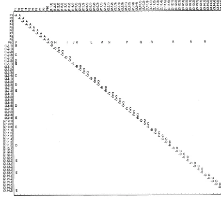
Figure 1 contains the complete rate matrix for the case study. The first 10 rows and columns are the productive states of the system (p1 – p10). Of
key importance is row 10 of the rate matrix. This row represents the final stage of the Erlang productive cycle time model. It is at this point, when the system must make the transition out of the 10-th stage, that the system can reenter the productive cycle time model or enter one of the {Ni, Dj, Ek} delay states. Given that the Pr[No
delay] = 0.571, the system will reenter the productive cycle time model 57.1% of the time and will enter one of the delay sequences 42.90% of the time. However, since the entries in the rate matrix are rates of change of probability, the probability must be transformed to rates. Two properties of rate matrices, mentioned earlier, can be used to accomplish this:
1. Row sums of the rate matrix must be zero. 2. The diagonal terms (i.e., denotes cases where
the system remains in the current state) are the negative of α from the Erlang model.
In this particular case, the entry in {p10, p1} is –
2.942. Then, the rate of change for moving from p10 to p1 is calculated as 2.942 times the probability of no delay (0.5721), which equals 1.6821. This, then, becomes the entry in { p10, p1 } of the rate matrix.
The rate matrix entries for moving into one of the
delay states are somewhat more difficult to calculate. The general procedure is to take the absolute value of the diagonal term (i.e., 2.941) times the probability of that one, two or three delays occurred (whichever case applies) times the probability of the particular delay type occurring. The procedure is best illustrated by using examples.
Assume that the next transition is to {p10, (1, 1, 1)}.
The cell entry is then 2.941 times the probability of one delay (i.e., 0.335) times the probability of delay type 1 (i.e., 0.257), which equals 0.253. For the cases in which two delays occur the procedure is exactly the same. Assume that the next transition is to {p10, (2, 2,
1)}. The entry in {p10, (2, 6, 1)} is 2.941 times the
probability of two delays (i.e., 0.089) times the probability of delay type 6 (i.e., 0.217), which equals 0.570.
Several additional items need clarified at this point. Once the system has move through a delay sequence, it always returns to p1 the first
productive stage of the cycle. When the system must move through a multiple delay sequence, it is assumed for the sake of simplicity that the sequence begins with the lowest numbered delay type. Once the system moves through the stage of that delay it immediately enters the first stage of the next highest numbered delay type. For example if delay type 1 and 2 occur, it is assumed that the system moves through the Erlang stage of delay type 1 first, followed by the 3 stages of delay type 2. It would make no difference in the results if the sequence were reversed.
Results Of The Case Study
The developedrate matrix used in equation (5) to solve for the steady state proportions of productive and delay time. Although the rate matrix is theoretically singular, it is possible to solve the system of equations by recalling that the steady-state probabilities must sum to one. Using this fact, solution of the system is handled by setting one row (or column) of the rate matrix to 1’s and setting the appropriate right-hand side element of the zero vectors to a 1. The system was solved using the PROC MATRIX procedure in SAS and the resulting steady-state probabilities were:
Pr[System in delay type 3] = 0.052 Pr[System in delay type 4] = 0.116
These probabilities were determined by summing over all states for each delay type and for each of the productive states. That is, the steady-state probabilities for each of the 10 productive states were summed to obtain the proportion of total time spent in a productive mode of operation. Based on these results, the system was productive almost two-thirds of the time, while the
remaining third was tied up in delay time, with hang-ups and miscellaneous delays occupying the majority of steady-state delay time. It is interesting to note that while the probability of miscellaneous delays was relatively low, it was more than offset by the distribution of time spent in a miscellaneous delay (as evidenced by the high average time) giving it the highest proportion of steady-state time.
productivity should initially focus on reducing the frequency of delays overall and to specifically focus on reducing the probability of hang-ups and miscellaneous delays.
One feature of Markov process models is that they allow the analyst to test the effects of various system adjustments without having to first implement them on the job. For instance, suppose the logging contractor could alter the probabilities of delays occurring, through a change in the mode of operation, as follows:
Pr[No delay] = 0.651 Pr[One delay] = 0.272 Pr[Two delays] = 0.074 Pr[Three delays] = 0.003
The steady-state probabilities resulting from this modification were:
Pr[System is productive] = 0.708 Pr[System in delay type 1] = 0.092 Pr[System in delay type 2] = 0.065 Pr[System in delay type 3] = 0.045 Pr[System in delay type 4] = 0.095
In this case the percentage increase in the proportion of productive time (about 6.8%) may not be justified since it required a 13.6% increase in the probability that no delay occurred. The cost of reducing the occurrence of delays may be greater than the savings resulting from the increase in steady-state productive time. For the operator, actual implementation of this change or any other change must be considered in light of any additional cost associated with such changes and the impact on the overall financial performance of the operation.
In making modifications, the operator or analyst can focus on two components of the system:
1. Reducing delay time for any given type of delay, which will alter the Erlang model of time-based activities for that delay.
2. Reduce the probability of occurrence of a delay type or the occurrence of delays in general, as illustrated in the above example
.
Either type of reduction should reduce the steady-state proportion of delay time for the
system. A third alternative may be to increase the productivity of the system, which will alter the productive time Erlang distribution. However, speeding up production beyond the capability of the system may cause an inordinate increase in delay time and presumably increase costs beyond acceptable levels.
The question, however, always remains: What is the most cost effective alternative available? Fortunately, the Markov model can be easily adapted to handle modifications in system components and to provide steady-state solutions to these modifications in a straightforward manner.
SUMMARY
This study was designed to illustrate the use of Markov process theory to the analysis of steady-state proportions of production and delay time of cable logging systems. The study was successful in that a stochastic model was developed and steady-state results were generated for each system. Of at least equal importance was the demonstration that stochastic models are viable tools for timber harvesting systems analysis.
A relatively elementary Markov process model that is both powerful and relatively easy to use was adapted to a relatively complex logging system. Yet, utilization of this model requires only elementary statistical tools for fitting Erlang distributions, some basic understanding of probability, and basic matrix algebra to solve systems of simultaneous algebraic equations. Solution of the model provided stead-state results for the proportions of productive and delay time. It was also shown how flexible the model can be for investigating the effect of possible modifications to the system.
REFERENCES
1. Blinn, C. R., “The Economics of Integrating the Harvesting and Marketing of Eastern Hardwood Timber to Achieve Increased Profitability”, Ph.D. Dissertation, VA, (1996),.208p. 2. Clarke, A. B. and Disney, R. L., “Probability and Random
Processes: A First Course with Applications”, J. Wiley and Sons, Inc., New York, (1992), 325p.
3. Conover, W. J., “Practical Nonparametric Statistics”, J. Wiley and Sons, New York, (1998), 495p.
5. Karlin, S. and Taylor, H. M., “A First Course in Stochastic Processes”, Academic Press, NY, (1992), 558p.
6. Mason, R. L., Tracy, N. D. and Young, J. C., “Development of Statistical Control of Correlated Variables”. ASQC Quality Congress Transactions, Milwaukee, (1998).
7. Seth, S. K. and Shukla, G. K., “Population Dynamics of Forest
Stands Stochastic Approach”, Indiana For. 98, (1996). 71-81. 8. Snedecor, G. W. and Cochran, W. G., “Statistical Methods.
The Iowa State University Press”, Ames, Iowa, (1999), 508p. 9. Peden, L. M., Williams, J. S. and Frayer, W. E., “A Markov