Continuous User Authentication via Random Forest

Fall 2018

Continuous User Authentication via Random Forest

Continuous User Authentication via Random Forest

Ting-wei Chang

Iowa State University, [email protected]

Follow this and additional works at: https://lib.dr.iastate.edu/creativecomponents

Part of the Other Computer Engineering Commons

Recommended Citation Recommended Citation

Chang, Ting-wei, "Continuous User Authentication via Random Forest" (2018). Creative Components. 49. https://lib.dr.iastate.edu/creativecomponents/49

Ting-Wei Chang

A thesis submitted to the graduate faculty

in partial fulfillment of the requirements for the degree of

MASTER OF SCIENCE

Major: Computer Engineering

Program of Study Committee: Daji Qiao, Major Professor

The student author, whose presentation of the scholarship herein was approved by the program of study committee, is solely responsible for the content of this dissertation/thesis. The Graduate College will ensure this dissertation/thesis is globally accessible and will not permit alterations

after a degree is conferred.

Iowa State University

Ames, Iowa

2018

DEDICATION

I would like to dedicate this thesis to my parents, without their support I would not have been

able to complete this work. I would also like to thank my major professor Dr. Qiao for his patient

TABLE OF CONTENTS

Page

LIST OF TABLES . . . v

LIST OF FIGURES . . . vi

ACKNOWLEDGMENTS . . . vii

ABSTRACT . . . viii

CHAPTER 1. Introduction . . . 1

CHAPTER 2. Background . . . 3

2.1 Random Forest . . . 3

2.1.1 Decision tree . . . 3

2.1.2 Bagging . . . 4

2.1.3 Algorithm of random forest . . . 4

2.1.4 Others properties of random forest . . . 5

2.2 Principle Component Analysis(PCA) . . . 6

2.3 Synthetic Minority Oversampling Technique(SMOTE) . . . 6

CHAPTER 3. Application of Random Forest . . . 8

3.1 Threat model . . . 8

3.2 System model and definition . . . 9

3.3 Design goal . . . 10

3.4 Methodology . . . 11

3.4.1 Data preprocessing . . . 12

3.5 Behavior Feature Extraction . . . 13

3.6 Random Forest for Learning and Classification . . . 15

3.6.1 Behavior Feature Classifier . . . 15

CHAPTER 4. Evaluation . . . 17

4.1 System performance . . . 18

4.1.1 Parameter Setup . . . 18

4.1.2 Performance Metrics . . . 18

4.1.3 Accuracy . . . 19

4.1.4 Delay of Detection . . . 20

4.2 Effect of Models and Parameters . . . 21

4.2.1 Effect of Size ofn-action-gram . . . 21

4.2.2 Effect of Feature Reduction and SMOTE . . . 22

4.3 Discussion . . . 23

4.3.1 Scalability of User Pool . . . 23

4.3.2 Comparison with other machine learning techniques . . . 24

LIST OF TABLES

Page

4.1 Area under curve(AUC) and equal-error rate (EER). The values are the

mean of 50 users . . . 19

4.2 Equal-error rate (EER) for differentnin n-gram. The values are ”mean(standard

deviation)” . . . 22

4.3 Dimensions ofn-action-gram behavior feature vectors before and after

fea-ture reduction. . . 22

LIST OF FIGURES

Page

2.1 Overview of random forest. . . 4

3.1 An example snapshot of a system log. . . 9

3.2 A generic model of user interactions with a software system. . . 10

3.3 Two-step user authentication with our proposed monitoring engine. . . 11

3.4 Overview of the proposed behavior and context monitoring engine. . . 12

3.5 An example global 2-action-gram feature space G under the activity se-quence model. In this example, d= 15 unique 2-action-grams are present in the training data. . . 15

4.1 Average ROC curve of 50 users. . . 20

4.2 EER of all users versus the number of observed actions. Upper line is maximum, upper bound of the box is 75% quantile, line in middle is median, lower bound of the box is 25% quantile, lower line is minimum, and the circles are outlier. . . 21

4.3 Example of legitimate user. . . 22

4.4 Example of imposter. . . 23

ACKNOWLEDGMENTS

I would like to take this opportunity to express my thanks to those who helped me with various

aspects of conducting research and the writing of this thesis. First and foremost, Dr. Daji Qiao for

his guidance, patience and support throughout this research and the writing of this thesis. I would

also like to thank Shen Fu for his help during this work, he gave many advise which inspire me to

ABSTRACT

Random forest is an important technique in modern machine learning. It was first proposed in

1995, and with the increasing of the compute power, it became a popular method in this decade.

In this paper, we present the background knowledge of random forest and also have comparison

with other machine learning methods. We also have some discussion of data preprocessing and

feature extraction. Then we study the application of random forest to a real world problem - an

authentication system which for continuous user authentication approach for web services based on

the user’s behavior. The dataset we used for evaluate is given by Workiva company, and the result

CHAPTER 1. Introduction

There has been plenteous interest in ensemble learning in recent year methods which has been

study by using multiple learning algorithms and aggregate their results to obtain better predictive

performance. Two most popular methods are bagging [1] and boosting [8] of classification trees.

Bagging stands for bootstrap aggregation, which reduce the variance of an estimate is to average

together multiple estimates. This can be implied that trees do not depend on earlier trees, each

bootstrap sample of the data set is independently constructed. The main principle of boosting is to

fit the decision trees to weighted versions of the data that are able to convert to stronger learner.

Then the predictions combined through a weighted majority vote to produce the final prediction.

[6] had first proposed the random decision forests using the random subspace method, which

implement the stochastic discrimination approach to classification. [1] introduced an extension of

the algorithm, it combines the idea of bagging and random selection of features. Random forest is

constructed by each tree using a different bootstrap sample of the data, which is only a subset of

the predictor variables is used. In each tree, nodes are split using the best split among all variables.

Then random forest using the best split among a subset of predictors to split the node. This

strategy gives random forest an outstanding performance even if compare to other classifiers, such

as support vector machine(SVM), nave bayes and K-nearest neighbor. Moreover, random forest

is flexible, easy to use machine learning algorithm that has only two hyper-parameter tuning (1)

Number of trees in the forest. (2) Number of variable in the random subset at each node. The

simplicity and the fact that it can be used for both classification and regression tasks makes the

random forest become one of the most used algorithms. The advantage of RF compare to other

classifiers are listed as follows:

• Runs efficiently on large data

• Give in formation about the relation between the variable and the classification.

• Little influence by the outlier and bad feature

The rest of this paper is organized as follows. In the chapter 2, we introduce the background of

random forest and compare it with other classifiers. Furthermore, we also introduce two methods for

data prepossessing which we have used in this paper. We discuss our main objectives, methodology

and the application of random forest in a real world problem is proposed in chapter 3. In chapter

4, we show the evaluation and discussion for our result. In chapter 5, we conclude the result and

CHAPTER 2. Background

2.1 Random Forest

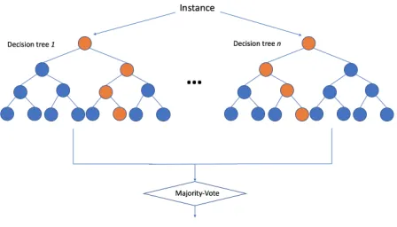
Random Forest is a supervised learning algorithm. The main idea of random forest is ensemble

many of decision tree to make a better prediction.

2.1.1 Decision tree

Decision tree is a decision support tool that uses a top-down tree-like model. Each internal

node in the tree represents a verification on an attribute, each branch represents the outcome of

the verification, and each leaf node represents a class or label. Generally, the decision trees are

used in operation research and calculating conditional probabilities, it should be paralleled by a

probability model as a best choice model.

There are 3 kinds method that we commonly used for decision tree, ID4, C4.5, CART. When

we building the tree, we need to extract the features from data as decision nodes. The principle

of choosing the features is that the features we chose can separate the different classes as much as

possible, this can be estimated by information gain, Gini coefficient, etc.

Pruning Optimal size of the final tree is one of the critical questions in the decision tree

algorithm. If the decision tree is too small, it might not capture the important information about

the data space. On the other hand, if the decision tree is too large, there might cause a problem

of overfitting on the training data and poorly generalizing to new samples. Nonetheless, it is

difficult to tell when to stop when growing a tree because it is impossible to tell if the addition

of a single extra node will significantly decrease error. This kind of issue is known as the horizon

contains a small number of instances, then use pruning to remove those nodes which do not provide

sufficient information.

Figure 2.1 Overview of random forest.

2.1.2 Bagging

Bagging, also called bootstrap aggregating is a technique for ensemble learning. The main

purpose of this method is to reduce variance and helps to avoid over-fitting problem. Here we use

bagging to the tree learner, given a training dataX =x1, , x2 and corresponding labelY =y1, , yn,

bagging repeatedly selectskrandom sample with replacement and fits trees to these samples. After

training, predictions for testing sample x can be made by taking the majority vote in the case of

classification trees.

Simply training many trees on a training data would give strong correlated trees. Bootstrap

sampling is a way to de-correlating the trees, which means even though the prediction of single tree

is sensitive to outliner or noise, the average of the forest is not. The procedure of bagging leads to

a better performance because it reduces the variance of the model without increase the bias.

2.1.3 Algorithm of random forest

The algorithm of random forest is quite easy to understand and simple as follows:

the best split among all predictors, we randomly sample mtry of the predictors and choose

the best split from among those variables.

3. Predict testing data by aggregating the predictions ofntree trees. (majority vote)

2.1.4 Others properties of random forest

Out of bag(OOB) In the training process, each tree is bootstrap from data which allow the

rest of the data consider as the testing set, this is called out-of-bag(OOB) sample. The excluded

OOB sample is used to evaluate the performance of the random forest in training by estimate the

mean square error(MSEOOB):

M SEOOB=n−1 n X

i=1

(yi−yˆiOOB)2 (2.1)

Where ˆyOOB is the average of the OOB predictions for the ith observation. The result of a

random forest is one single prediction which is of the average over all aggregations. The evaluation

of OOB has been proved is quite accurate, given that enough trees have been grown. (Bylander

2002)

Variable importance Random forest can be used to rank the importance of variables in

classification problem. The following methods has been described in Breimans paper. First, we

fit random forest to the training data, then the OOB error for each data point is recorded and

averaged over the forest during the fitting process. Then the importance score for the features are

computed by averaging the difference in OOB error before and after the permutation over all trees.

The score is normalized by the standard deviation of these differences. Features which has higher

score are ranked as more important than the features which has smaller value. However, there

are some drawbacks of determine the variable importance. For those data including categorical

variables with different number of levels, random forest are biased in favor of those attributes with

2.2 Principle Component Analysis(PCA)

The curse of dimensionality is one of an important is- sue in the data processing. One of the

solution is data extraction, mapping the data into a lower dimension. Extracting the data from a

higher dimension to a lower dimension not only can improve the performance of the classifier, but

also can reduce the data size. In this paper, principle component analysis(PCA)[7] is used to convert

our data into a set of values of linearly uncorrelated variables. PCA is mathematically defined as

an orthogonal linear transformation, it transform the largest variance of feature in the data comes

to lie on the first coordinate, also called the first component, and so on. For a p-dimensional data,

the transformation is defined as a set of weights vector, wk= (w1, w2, ..., wp)k that map each row

vectorx_(i) of X to a new vector of principle component scorest_(i)= (t1, t2, ..., tm)

tk(i) =x(i)·w(k)f or i= 1to n, k = 1to m (2.2)

To maximize the variance, the first vector

wi = argmax X

i

(t1)2(i), (2.3)

sincew(1) has been defined as a unit vector

wi = argmax

wTXTXw

wT_w , (2.4)

After we find the w(1), the first principle component of a data vector x(i)can be given as t1(i) =

x(i) ·w(1)in the transformed co-ordinates. The further components can be found in the same

method.

2.3 Synthetic Minority Oversampling Technique(SMOTE)

Learning from the imbalanced data can cause suboptimal classification performance. In the

previous works, a number of solutions to the imbalance problem were proposed. The simplest

dataset, solution includes adjusting the threshold of various classes, adjusting the costs of different

classes. The synthetic minority oversampling technique(SMOTE) [2] is one of the solution to the

imbalance data. SMOTE oversampling the minority by creating synthetic example along the line

segments in feature space, then joining any of the n nearest neighbors which is also minority class.

The amount of oversampling is influence by the number of randomly selected neighbors from the n

nearest neighbors. For the majority class, it is undersampled by randomly removing samples until

CHAPTER 3. Application of Random Forest

In this paper, we propose a method to implement random forest to a continuous authentication

software systems. The framework features a monitoring engine that supplements and enhances

the standard two-step authentication architecture used by companies such as Google, Facebook,

Twitter, etc.

The goal in this section is to indicate a) what kind of problem and scenarios our authentication

framework mainly focus on b)Introduce all the definitions in this system c) Define what kind of

dataset can be used for training in our framework, and d) the design goals we expect our approaches

to achieve.

3.1 Threat model

In practice, most software systems only perform user authentication when a user logs in to the

system. Once an attacker passes the initial authentication, the attacker has complete control and

access to the user’s account. Clearly, password authentication is not sufficient for our threat model,

and another layer of protection is needed to deal with these impostor attacks.

The software system discussed above may experience various types of attacks. In this work,

we focus onimpostor attacks, with impostor defined as an illegitimate user who accesses a system

by pretending to be a legitimate user. In our threat model, an impostor may attack in one of the

following ways:

Obtaining credentials (software level) The impostor obtains the password or other login

device, such as a workstation, that is already logged into the system by a legitimate user.

3.2 System model and definition

In this work, we consider a generic software system as follows.

• Each user account in the system has a username as its unique identifier and a password

needed to log into the account.

• After users log in, they interact with the software system by performing a stream of operations,

such as read, write, change, and more.

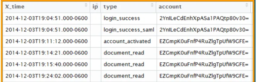
• Each user’s operation stream is recorded in a system log as a sequence of tuples consisting

of system time, operation type, and additional information. Figure 3.1 shows part of a real

system log provided by Workiva.

Figure 3.1 An example snapshot of a system log.

Action: Theaction of a user’s operation is a categorical variable clearly describing the

oper-ation type. The action is the major feature representing the user behavior in an operoper-ation stream.

”doc-ument read” in Figure 3.1. In some systems, the action is not explicit and needs to be extracted

from the operation stream as part of data preprocessing.

Session: A session is a section of an operation stream. In our approach, session is a general

concept, not a specific application term. We partition the operation stream into sessions based on

either explicit login/logout operation, or long idle-time intervals (timeouts). We classify users based

on sessions, instead of considering the entire operation stream, to make computations manageable.

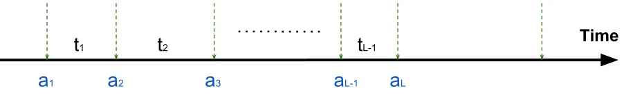
Our target software system could be hosted locally or remotely. Figure 3.2 shows a generic

model of interactions with such a software system, whereai denotes the action of theithoperation

of a session andti denotes the time interval between operations iand i+ 1.

Time

login

read

browse

write

logout

a

a

a

a

a

t

t

idle

login

t

Figure 3.2 A generic model of user interactions with a software system.

3.3 Design goal

To deal with impostor attacks, we introduce an monitoring engine into the common two-step

user authentication framework. As shown in Figure 3.3, our monitoring engine sits between the

first authentication and the second authentication. The engine monitors the user’s behavior

con-tinuously, comparing it with a pre-established user profile. If the user’s behavior or context differs

from normal, our monitoring engine raises an alarm, triggering the second step of authentication.

The design goals for our monitoring engine are to:

• Provide continuous user authentication to defend against impostor attacks.

• Detect impostors quickly after the intrusion occurs.

(FRR) and false-acceptance rate (FAR).

Figure 3.3 Two-step user authentication with our proposed monitoring engine.

3.4 Methodology

Figure3.4shows an overview of our behavior monitoring engine. The engine is broken down into

four modules: thedata preprocessing module, thefeature extraction module, thelearning

module, and the classification module. The data preprocessing module adapts the users’ raw

data (operation stream) for our engine and partitions it into sessions. In the training process, the

feature extraction module determines the behavior information features of each user and passes

them to the random forest training for profile establishment. In the testing process, the feature

extraction module passes the features of operations to the classification module in real-time, which

assigns a risk score that estimates the probability that the current session belongs to an impostor.

The risk score is converted into a binary result (impostor or not) by comparing it to a discrimination

threshold. In the remainder of this section, we describe our preprocessing, feature extraction, and

Figure 3.4 Overview of the proposed behavior and context monitoring engine.

3.4.1 Data preprocessing

Real-world data is often incomplete, inconsistent, and noisy. Good data preprocessing not only

makes the data usable, but also increases the performance of the system. The details of data

preprocessing are usually data-dependent, so here we only discuss general data preprocessing that

is appropriate for a typical dataset used in our approach. We outline two main steps: preprocessing

the operation stream, and extracting sessions.

The raw data of users in our system is expected to be a stream of categorical variable tuples,

usually including timestamp, operation type, user identification, and more. In this step, we remove

tuples which are meaningless operations or are not generated by the user. For example, consider

a tuple with operation type ”logout−timeout,” generated by the system automatically after the

user does not perform any operations for an amount of time. This tuple does not provide useful

the following ”logout” operation. However, in our experience, many users of software systems such

as web services do not logout manually. These users either let the system automatically logout due

to timeout, or perform operations regularly enough to remain logged in indefinitely. Therefore, we

use time-stamps as a supplemental method for extracting sessions. In this method, if a user does

not perform any operations for a certain length of time, we consider the previous operation tuple to

be the end of the session and consider the next operation tuple to be the start of a new session. Our

behavior feature extraction procedure consists of two steps: construction of a categorical variable

sequence for each session, and generation of a numeric feature vector representing each of the

sequences.

3.5 Behavior Feature Extraction

In this step, we transform the tuples from preprocessing into a sequence of categorical variables.

We propose two different models for this transformation: an activity sequence model, and a ”hybrid”

model that utilizes both activity sequences and time intervals.

Activity Sequence Model: In the activity sequence model, a session is represented as a

sequence of actions sorted by order of arrival. This model can distinguish legitimate users and

impostors if they focus on different activities and have different activity transition patterns.

For-mally, given the set of allrpossible operation typesO={type1, type2, ..., typer}, using the activity

sequence model, the sequence S of one session with L actions is S = (a1, a2, a3, ..., aL), where

ai ∈ O is the ith action of the user in the session. For example, if the operation stream in

Fig-ure 3.1 is a complete session, the behavior sequence of this session using the activity sequence

model is S = (login success, login success saml, account activated, document read, document read,

document read).

Hybrid Model: In the hybrid model, we consider both the order of actions in a session and

except between each pair of consecutive actions, we insert an additional entry that represents the

time between the actions. Formally, the sequence is S = (a1, t1, a2, t2, ..., aL−1, tL−1, aL), where

ai∈O is as before, andti is the time between ai andai+1. To apply this model in our framework,

ti must be a category value. We obtain category values from integer time values (e.g. seconds) by

placing the integer time values into log-scale buckets and mapping each bucket to a category index

number. Specifically, we map an integer time valuet to the categorytdiscrete as follows:

tdiscrete= [log10(t)], f or t >0, (3.1)

and tdiscrete = 0 for t= 0. With this method, the sequence S contains only categorical variables,

as in the activity behavior model. Again using the operation stream in Figure 3.1 as an example

session, the behavior sequence using the hybrid model isS = (login success, 0, login success saml,

3, account activated, 3, document read, 2, document read, 3, document read).

3.5.1 Generating a Numeric Feature Vector

In the second step of behavior feature extraction, n-action-gram representation is used to

gener-ate a numeric feature vector from each sequence. To do this, we first need to determine the globaln

-action-gram feature space. Given a sequence under the activity sequence modelS= (a1, a2, ..., aL),

the set of all types of n-action-grams (consecutive action subsequences of length n) appearing in

the sequence is denoted A(S). For the hybrid modelS = (a1, t1, a2, t2, ..., aL), eachn-action-gram

also includes the n−1 time intervals between the actions, for a total length of 2n−1 for each

subsequence. Suppose that duniquen-action-gram subsequences are present in the training data,

and assume that these d subsequences are all of the subsequences that will occur in practice.

Then, given the data sequences S1,S2, ..., SM, the global n-action-gram feature space is defined

as G = MS i=1

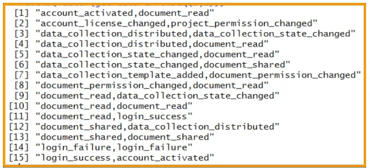
A(Si) = {b1, b2, ..., bd}, where bj is one type of n-action-gram. An example global

n-action-gram feature space is shown in Figure3.5.

Finally, for each sequence, we use a numeric vector~vof fixed lengthdto represent the sequence,

vi =

q(bi)

Pd

j=1q(bj)

, (3.2)

where q(bi) is the count of n-action-gram types bi in the sequence. Note that, after representing

each behavior sequence as a vector, the distance between two sequences can be computed as the

Euclidean distance of their feature vectors.

Figure 3.5 An example global 2-action-gram feature spaceG under the activity sequence model. In this example, d = 15 unique 2-action-grams are present in the training data.

3.6 Random Forest for Learning and Classification

This section describes how random forest learning and make the real-time classification. The

random forest use behavior information features defined above.

3.6.1 Behavior Feature Classifier

The monitoring engine is based on random forest classifier which use behavior feature as training

data. The training process can be divided in to 3 steps:

Step 1. Before learning, we bind the behavior feature vectors of all sessions of training data

lower-dimensional approximation of the data. PCA converts data into a set of scores corresponding

to different linearly uncorrelated variables (principal components). After PCA, we recreate the

feature space while ignoring all principal directions with a standard deviation of corresponding

principal scores less than 1% of the top principal direction. In this way, the number of feature

dimensions is greatly reduced. For example, in our evaluation, feature dimensions were reduced

from 1,214 to 540 when using the 2-action-gram hybrid sequence model.

Step 2. Training datasets for our monitoring engine can be greatly unbalanced. Usually, much

more of the data is from legitimate users than impostors, though in some situations, the opposite can

be true. Either way, learning from this unbalanced data can lead to poor classification performance.

We use the Synthetic Minority Oversampling Technique (SMOTE) [2] to deal with this issue. The

SMOTE algorithm generates a new, balanced dataset. SMOTE over-samples each minority class

sample by creating synthetic examples along the line segments joining all of the sample’skminority

class nearest neighbors. At the same time, SMOTE under-samples the majority class data.

Step 3. The balanced data generated by SMOTE is passed to random forest classifier then

starts training. The training result for each user will save as an”user profile”.

In the testing process, given the input session of a particular user into his user profile, the

classifier returns a behavior-based risk score. The risk score is computed as the fraction of decision

trees that classify the input session as belonging to an impostor.

If an impostor successfully logs into the system and starts performing operations, the monitoring

engine should raise an alarm as soon as possible. Therefore, in practice, the behavior risk score is

computed based on all operations in the current session and is updated whenever a new operation

CHAPTER 4. Evaluation

In this work, we want to evaluate how random forest perform for our approach on a real dataset

given by a Workiva which provides a cloud platform for reporting, compliance and data management

services. For each user in the dataset, his/her operation stream over the course of a month has been

recorded in the form of tuples with six categories: ”time”, ”IP”, ”operation type”, ”account

ID”, ”user ID”, and ”document.” We extract the n-action-gram behavior features from the

sequence of ”operation type,” while ”time” and ”IP” are used as context features in our approach.

Each day is divided into 4 intervals.

Insufficient of history data from some of the users has been found from our observation, which

can lead to an inaccurate prediction. Therefore, we chose the users who participated over 15 days

in a month, and contributed a variety of actions among the dataset. That is roughly 50 users match

the condition. In each scenario, we assume there is only one legitimate user, the other 49 users

are consider as impostors. One of the significant distinction between this work and most of the

previous work is that our dataset does not contain any data from real impostors. Therefore, we

evaluate our authentication system for each user by using the data of other users as impostors (i.e.

1 versus 49). This is a challenge for us, because the behavior from legitimate users can be very

similar. For each user in the dataset, we select 30% of the user’s sessions as testing data, resulting

in 70% of the sessions being used for training.

Since the data of each user is a operation stream through the whole month and it’s obviously

not reasonable to make a classification based on the entire stream, we first divide the stream into

many meanful pieces in data pre-processing, called session. Then our classification can be based

on sessions. The simplest way to define session is consider the interval between ”login success” and

”logout success”. However, according to our experience, most of the user don’t logout manually.

the time stamp as the condition to define the session of actions is more reasonable. Thus we use

60 minutesas the idle to separate sessions, as shown in Figure3.2.

4.1 System performance

4.1.1 Parameter Setup

For our evaluation, we implemented our proposed framework in the R language. In the data

preprocessing module, we use 60 minutes as the idle interval to separate sessions. In the

behavior-based classifier, by default we use the 2-action-gram hybrid model. In this work, we use random

forest (RF) as our behavior-based classifier.

There are 2 parameter that we need to tune for the random forest: number of trees(ntree) and

number of features for splitting at each tree node(mtry). Large number of trees produce more

stable models and co-variate importance estimates. However, it will require more memory and

longer running time. It has been discussed by [10] and proved that 500 trees is sufficient for a large

dataset, so we set ntree to 501. There is some discussion in the literature about the influence of

mtry. (Cutler 2008) claimed that different values of mtry did not affect the correct classification

rates of their model and other performance metrics such as AUC, ROC, etc., were stable under

different values of mtry. On the other hand, [10] reported that mtry has a strong influence on

predictor variable importance estimates. Generally, people tends to avoid the correlation of each

features, which recommend using less number of features in each tree such as 3/mor√m. In this

paper, we use √mas our mtry.

4.1.2 Performance Metrics

ROC Curve and AUC The receiver operating characteristic (ROC) curve [5] is a universal

metric for classifiers that output a probability score, making it a good choice for evaluation. The

ROC plots the true positive rate (TPR) against the false positive rate (FPR) of a binary classifier

approaching 1.0 indicates perfect performance of a classifier.

EER The error rate of a classifier characterizes how often the classifier correctly classifies

testing samples, making it more intuitive and easier to understand than the ROC curve and AUC.

We use equal-error rate (EER) [9] as our system metric instead of (ordinary) error rate, due to the

fact that our dataset is heavily unbalanced for two-class classification (one legitimate user versus

49 impostors). EER provides a better measure of our framework’s performance; for example, if the

classifier predicts all the testing samples to be majority class, the (ordinary) error rate can be very

low, but for our unbalanced dataset, this does not mean the classifier has good performance. EER

can be easily computed from the ROC curve by finding the point at which FPR is equal to the

false-negative rate (FNR).

Delay of Attack Detection For a real-time authentication system, another important metric

is the delay before an attack is detected, meaning the time between an impostor’s login and the

alarm raised by the system. The delay of attack detection can be represented as EER versus the

number of observed actions.

4.1.3 Accuracy

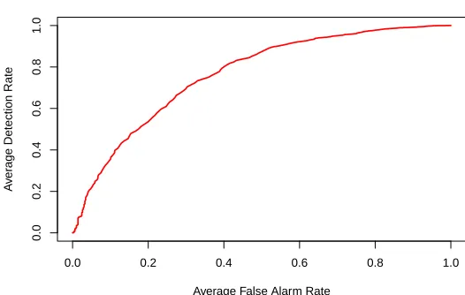
Figure 4.1 shows the average ROC curves of all users. The details of the ROC curves can be

found in Table 4.1. Most of the user in this work has achieved 0.7751 in AUC, however, some of

the users are difficult to classify, this kind of the users will be discuss later in this chapter.

Average Standard Deviation

Area Under Curve 0.7751 0.0238

Equal-Error Rate(%) 25.76 10.97

Average False Alarm Rate

A

v

er

age Detection Rate

0.0 0.2 0.4 0.6 0.8 1.0

0.0 0.2 0.4 0.6 0.8 1.0

Figure 4.1 Average ROC curve of 50 users.

4.1.4 Delay of Detection

To make our system more practically useful, our monitoring engine should be able to quickly

detect an impostor. In this section, we evaluate how many actions are required to accurately classify

legitimate users and impostors. We expect the EER to decrease quickly at the beginning, as the

number of observed actions increases, and eventually become stable.

To evaluate the delay of detection, we use testing data to simulate real-time users. Given a

testing session as described in Section 3.5.1, we first consider only the first two actions of the

sequence and the time interval between them for behavior feature extraction. This simulates the

situation where the user has only finished two actions in the session. Then we repeat this process

using the first three actions and corresponding time intervals, and so on. In each iteration, the

results of the context classifiers do not change, but the behavior classifier does, influencing the final

risk score. With this evaluation method, the output of a testing session can be represented by a

sequence of risk scores versus the number of actions which the user has finished.

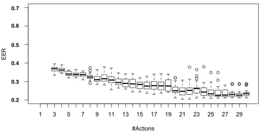
Figure 4.2 shows the EER of all users as the number of observed actions increases. As can

be seen in the figure, the EER stabilizes at around 20 actions, meaning after a user logs in and

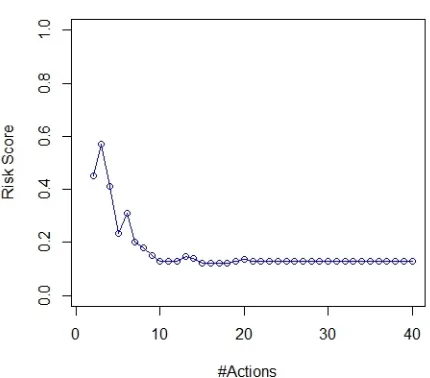
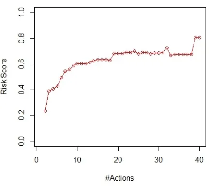
the number of actions in a session of a legitimate user, and the risk score decreases quickly as more

actions are observed. For comparison, Figure4.4shows an impostor session. With a discrimination

threshold of 0.5, this particular impostor can only perform around seven actions before the system

raises an alarm, demonstrating the short detection delay of our system.

Figure 4.2 EER of all users versus the number of observed actions. Upper line is maximum, upper bound of the box is 75% quantile, line in middle is median, lower bound of the box is 25% quantile, lower line is minimum, and the circles are outlier.

4.2 Effect of Models and Parameters

4.2.1 Effect of Size of n-action-gram

To show the effect of the parameter nin then-action-gram representation method, we present

the performance of 2, 3, 4 and 5-gram methods in Table 4.2. The overall performance of 2-gram

and 3-gram is close, while 4-gram and 5-gram have worse performance, specifically, higher FRRs

and lower FARs. This indicates the system tends to become unbalanced and predict more users as

impostors whennbecomes larger. This is because when the length of the sequence becomes longer,

the probability that the exact same sequence happens again for a user becomes smaller. Thus, at

Figure 4.3 Example of legitimate user.

and be correctly accepted by the system. Therefore, in practice, we choose 2-gram or 3-gram for

behavior feature extraction.

n-action-gram 2 3 4 5

EER (%) 25.76 (10.97) 29.53 (11.45) 32.95 (15.21) 45.05(18.75)

Table 4.2 Equal-error rate (EER) for different n in n-gram. The values are ”mean(standard deviation)”

4.2.2 Effect of Feature Reduction and SMOTE

n-action-gram 2 3 4 5

# dimensions (original) 1214 5265 12377 19954 # dimensions (after PCA) 540 1242 1438 1375

Table 4.3 Dimensions of n-action-gram behavior feature vectors before and after feature reduction.

To demonstrate the effectiveness of feature reduction in our system, we present the number of

dimensions of the n-action-gram features before and after PCA in Table 4.3. As can be seen, PCA

Figure 4.4 Example of imposter.

FRR (%) FAR (%)

without SMOTE 74.49 10.19

with SMOTE 33.72 18.71

Table 4.4 Effect of the SMOTE algorithm

behavior classifier. Additionally, PCA has little effect on the classification results. The results in

Table4.2include PCA, and the results without PCA are not significantly different.

The SMOTE algorithm is also very important for our dataset. Without SMOTE, there are

approximately 50 times as many imposter (other user) sessions as legitimate user sessions. This

serious imbalance causes most sessions in our testing data to be classified as impostors, making

FRR very large while FAR is very small (see Table 4.4).

4.3 Discussion

4.3.1 Scalability of User Pool

In practice, we prefer to use data from real impostors for training rather than data from other

of the number of users in the system. However, since we use data from other users as impostors in

our evaluation, the size of the user pool may influence the results. Generally, when the user pool

becomes larger, the probability that some users are similar will increase, which may result in worse

classification accuracy. Therefore, in this section, we evaluate the scalability of the user pool in our

experiments.

To do so, we vary the size of user pool, u, between 2 to 50 with a step size of two. Given a

specific size of the user poolu =uk, we randomly sample uk users from all 50 users and compute

the average EER over these uk users. We repeat the process of sampling uk users 50 times, and

compute EER. Figure 4.5 indicates that as u increases, the mean EER first fluctuates some and

then gradually stabilizes, with u having only a slight effect on the performance when u is large.

Overall, these results indicate that the size of the user pool has only a slight effect on performance

above a certain size, and it has little effect on our experiments.

Figure 4.5 EER versus number of users.

4.3.2 Comparison with other machine learning techniques

In this work, we successfully implement random forest into a authentication system and give a

fair result. Other classifiers such as KNN or SVM are also suitable for our system, but we gives

method based on statistics theory. It is a theory that established on a set of finite samples. The

main idea of SVM is try to maximizes the margin for classes, thus it relies on the concept of

”distance” between different points. General problems such as linear analysis, small sample, local

minimum points, can be solved by SVM. However, SVM is less interpretable, it is difficult to explain

how the features effect the result. Random forest has better interpretability because we can look

into each node in the decision tree. Furthermore, the training for SVM takes more time and process.

For example, if the data has n points, than the SVM is constructing an n×n matrix. Therefore

SVM is hardly handle a large set of data.

K-nearest neighbors(KNN) K-nearest neighbors(KNN)[4] is a method that classify the

point by looking at its neighbors, and find the majority group. The number of neighbors is a

ad-hoc problem. KNN has some nice properties, it is non-linear by defult, and it tends to perform

well with a large among of data points. Nonetheless, KNN is highly sensitive to bad features and

outliers, thus KNN highly rely on the data prepossessing to make a better prediction. For the RF,

the features are randomly selected in each decision tree, hence the classification will not generate

a result which has affected by the outliers or bad features. Another drawback of KNN is that it

needs to calculate the distance between every each two data points, which means it calculaten2 _if

the data has n points, that makes the training process not very efficient.

Neural network Neural network is one of the most popular technique and has been studied

and applied successfully in many problem. The reason why neural network is so popular is because

a)it has the ability to learn and model non-linear and complex relationships. b)it is very flexible,

neural net work does not impose any restrictions on the input variables. c)it can be used for a

time series input. However, the training time for the neural network can be extremely long once

the neural network has a large number of neural and layers. Another drawback for neural network

dataset is too small. On the other hand, random forest can be trained with a small dataset and

CHAPTER 5. Conclusion and Future Work

We dealt the primarily with adversarial model with impostors in this experiment. Even so,

impostors detection is still a difficult problem. Our approach did not achieve very high detection

rate with a low alarm rate for every each user. This is partly because all of the users we used in

this experiment are legitimate user, most of them have a similar pattern of behavior, which can be

a handicap to the classifier. Another reason is the effect of diverse behavior. We believe that the

higher diversity of behavior will also have a higher accuracy. However, the users in our dataset are

concentrate in only 20 kinds of action even if the variety of the action in our dataset is 87.

One possible work in the future is gathering more data and evaluating on an expanded dataset.

We believe the performance of our authentication approach would benefit from an expanded dataset,

both in terms of length of user histories , and in terms of variety of users. In particular, we believe

data from real impostors would be highly beneficial.

A second possibility for future work is implement different classifier such as recurrent neural

networks(RNN), which have become more and more popular in recent years. RNN has been used for

solve the time sequence problem, that we can fit our action sequence in. However, neural networks

usually require a very large dataset to train, so our one-month dataset may be too small.

To draw a conclusion, we propose a generic framework of two-step user authentication approach

for general remote software systems. In the framework, we use multiple factors for authentication,

including password, behavior, and context information, and we also design a mechanism to

au-tomatically tell which users are applicable. Our approach has been evaluated on real users data

and our results show that the behavior and context monitoring engine achieves high accuracy of

classification and short detection delay. Furthermore, the mechanism to distinguish non-applicable

Since this approach is only based on user’s behavior, we can apply our work to generic web

ser-vice. The framework expands on the multi-factor authentication approach by integrating behavior

into authentication. We have proposed various mechanisms to make our framework more feasible

in practice, including dimensionality reduction and handling of imbalanced data. Our approach has

been evaluated on real user data and our results show that our behavior and context monitoring

Bibliography

[1] Breiman, L. (1996). Bagging predictors. Machine learning, 24(2):123–140.

[2] Chawla, N. V., Bowyer, K. W., Hall, L. O., and Kegelmeyer, W. P. (2002). Smote: synthetic

minority over-sampling technique. Journal of artificial intelligence research, 16:321–357.

[3] Cortes, C. and Vapnik, V. (1995). Support-vector networks. Machine learning, 20(3):273–297.

[4] Cover, T. and Hart, P. (1967). Nearest neighbor pattern classification. IEEE transactions on

information theory, 13(1):21–27.

[5] Fawcett, T. (2006). An introduction to roc analysis. Pattern recognition letters, 27(8):861–874.

[6] Ho, T. K. (1995). Random decision forests. In Document analysis and recognition, 1995.,

proceedings of the third international conference on, volume 1, pages 278–282. IEEE.

[7] Jolliffe, I. (2011). Principal component analysis. In International encyclopedia of statistical

science, pages 1094–1096. Springer.

[8] Schapire, R. E. and Freund, Y. (2012). Boosting: Foundations and algorithms. MIT press.

[9] Schuckers, M. E. (2010). Receiver operating characteristic curve and equal error rate. In

Computational Methods in Biometric Authentication, pages 155–204. Springer.

[10] Strobl, C., Boulesteix, A.-L., Kneib, T., Augustin, T., and Zeileis, A. (2008). Conditional