Some Geometrical Bases for Incremental-Iterative Methods (RESEARCH NOTE)

(1)

RESEARCH NOTE

SOME GEOMETRICAL BASES FOR

INCREMENTAL-ITERATIVE METHODS

M. Rezaiee-Pajand*, M. Tatar and B. Moghaddasie

Department of Civil Engineering, Ferdowsi University of Mashhad P.O. Box 91775-1111, Mashhad, Iran

[email protected] – [email protected] - [email protected]

*Corresponding Author

(Received: December 29, 2008 – Accepted in Revised Form: July 2, 2009)

Abstract Finding the equilibrium path by non-linear structural analysis is one of the most important subjects in structural engineering. In this way, Incremental-Iterative methods are extremely used. This paper introduces several factors in incremental steps. In addition, it suggests some control criteria for the iterative part of the non-linear analysis. These techniques are based on the geometric of equilibrium path. Finally, some examples illustrate the capabilities of suggested approaches.

Keywords Non-Linear Analysis, Incremental-Iterative Method, Control Method

! "# . # % #

& '( % )*+ % # % % ! , !-" . . /01 #

% +)2#+)2 # % )#*+ 3#2 %

4 & . 5* %

"*6 %

*- % ! & % 0& 7 # 8 .

'( 9

: !- + . 7 ; < +)*+ : . % % +) < <8+

!

& % 7 8 % /=. )-.

1. INTRODUCTION

Incremental-iterative methods are able to perform non-linear analysis for structural problems. These approaches can trace the equilibrium path by predictor and corrector steps. Most of the iterative techniques follow the classical Newton-Raphson procedure with some modifications. In this method, load factor remains constant during iterations. This makes the analysis divergent when it faces the limit points on the equilibrium path. In order to solve the mentioned problem, other criteria have been examined, such as displacement [1], work [2,3], residual energy [4], orthogonality [5] and so on. In this way, the comparison of various techniques could reveal the advantages and disadvantages of presented approaches [6,7]. One of the most applicable techniques is the Arc-Length Method. In 1979, Riks introduced the constant arc-length which could pass the limit and

turning points [8]. Subsequently, Crisfield modified Riks' approach and established the cylindrical arc-length method [9,10]. Afterwards, Fujii and Ramm investigated the path switching for bifurcation points in equilibrium paths [11]. For more simplification, the linearization techniques (e.g. orthogonality [5]) can be applied.

On the other hand, the incremental part plays an important role in analysis convergence. Selecting suitable parameters in predictor steps, could make an excessive impression on the rate of convergence, specially in highly non-linear problems [12,13]. For example, a proper extrapolation in the incremental part can avoid divergence [14,15]. Incremental-iterative techniques, as a solution of non-linear problems, are also able to combine with Neural Networks, Boundary Element Method and Normal Flow Algorithm [16-18].

(2)

incremental-iterative solution. Furthermore, several incremental factors are examined to obtain the compatibility between suggested techniques and incremental parameters. Section 2 describes the incremental-iterative procedure. Afterwards, various formulations for the corrector load factor are suggested in Section 3. The state of predictor step is shown in Section 4. Finally, a number of numerical examples are provided to evaluate the suggested methods.

2. THE INCREMENTAL-ITERATIVE METHOD

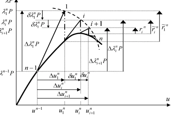
In this section, the structure of incremental-iterative analysis will be reviewed. As it is observed in Figure 1, the nth increment starts at equilibrium point (n−1).

First iterative point can be achieved by linearization:

P n 1 n 1 u 1 n

K − ∆ =∆λ (1)

Where, _Kn−1_{is the tangent stiffness matrix at}

) 1 n

( − , ∆u represents the incremental displacement, λ

∆ shows the incremental load factor and P is the external load vector. Superscripts and subscripts

indicate the number of increment and iteration, respectively. After each increment, iterative process begins. At this stage, n

i

δλ and n

i

u

δ ,

corrector load and displacement factors, are calculated and improve the incremental factors:

n i n

i n

1

i+ =∆λ +δλ λ

∆ (2)

n i u n i u n

1 i

u ₊ =∆ +δ

∆ (3)

In order to compute δuni, the following linear

problem should be solved:

n i r n i u n i

K δ = (4)

where, n i

r is the decreased residual force, and can be obtained by

P n

i n i r~ n i

r = +δλ (5)

In this equation, n i

r~ represents a residual force

vector. By substituting Equation 5 into (4), n i

u

δ can be computed as follows:

n i u n

i n i u n i

u =δ ′′ +δλ δ ′

δ (6)

(3)

Here, n i

u′′

δ and n

i

u′

δ have been produced by the residual force and external load, respectively:

n i r~ n i u n i

K δ ′′ = (7)

P n i u n i

K δ ′ = (8)

Equations 7 and 8 have no answers when the nth increment is located so close to a critical point. In order to overcome this problem, a coefficient should be considered beside the increment factor. As it is observed, another equation is needed to estimate n

i

δλ and complete the non-linear analysis process. It is needless to say that using a proper equation can have a great effect on the rate of convergence. There are many methods based on various assumptions to obtain a formula for δλni.

Most of these approaches have been extracted from the geometry of the load-displacement diagram. In 1981, Crisfield introduced one of the most reliable techniques in computation of the corrector load factor. He assumed that the length of n

1 i

u₊

∆ is constant for all iterations in each increment and it equals to the initial value Ln [9]:

n 1 u T n 1 u 2 ) n L

( =∆ ∆ (9)

2 ) n L ( n 1 i u T n 1 i

u ₊ ∆ ₊ =

∆ (10)

After substituting Equations 3 and 6 into (10), δλni

can be computed by solving Equation 11:

0 c ) n i ( b 2 ) n i (

a δλ + δλ + = (11)

n i u T n i u

a=δ ′ δ ′ (12)

n i u T ) n i u n i u ( 2

b= ∆ +δ ′′ δ ′ (13)

2 ) n L ( ) n i u n i u ( T ) n i u n i u (

c= ∆ +δ ′′ ∆ +δ ′′ − (14)

The mentioned approach is called The Cylindrical Arc-Length Method [9]. Because of simplicity in computer programming and adequate reliability,

this technique is excessively used in non-linear analyses.

3. ESTIMATION OF THE CORRECTOR LOAD FACTOR

There are many methods to procure a suitable formula for n

i

δλ . This section suggests some techniques which can be applied for highly non-linear problems.

3.1. Linearization of Arc-Length Method The cylindrical arc-length method leads to a second order Equation 10. It can cause some problems when one of two answers is selected. To avoid this, Equation 10 is replaced by the following equation:

2 ) n L ( ) n i u n 1 u ( T n i

u ∆ +δ =

∆ (15)

Where, L_n is obtained by using Equation 9.

Considering Equation 6, n i

δλ is available by a linear equation: n i u T n i u ) n i u n 1 u ( T n i u 2 ) n L ( n i ′ δ ∆ ′′ δ + ∆ ∆ − = δλ (16)

3.2. Orthogonality of n 1

u

∆ and n

i

u

δ One of the assumptions, that can lead to a simple formula for a corrector load factor, is to make an orthogonal condition between ∆u1n and

n i u δ : 0 n i u T n 1

u δ =

∆ (17)

By applying Equation 6, the value of n i

δλ will be in hand: n i u T n 1 u n i u T n 1 u n i ′ δ ∆ ′′ δ ∆ − = δλ (18)

(4)

analysis, is the residual length shown by n i

S in

each iteration. It is defined by summation of n i

u

δ and n

i r : n i r n i u n i

S =δ + (19)

Minimizing the value of the residual length is one of the techniques that results in a suitable formula for n

i δλ : 0 ) n i S T n i S ( = λ ∂ ∂ (20)

By substituting Equations 5, 6 and 19 into (20), the corrector load factor will be obtained:

) P n i u ( T ) P n i u ( ) P n i u ( T ) n i r~ n i u ( n i + ′ δ + ′ δ + ′ δ + ′′ δ − = δλ (21)

It is noteworthy that the load and the displacement have been divided by the length of the relative vectors at the first Predicator Step. Consequently, Equation 20 is dimensionless.

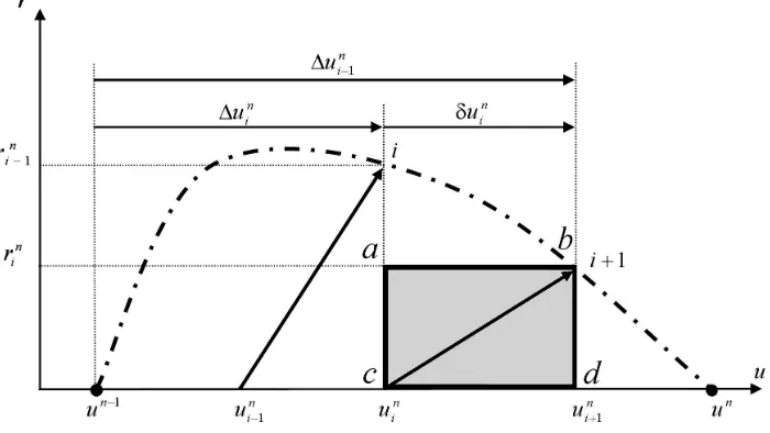
3.4. Minimizing the Residual Area The residual

area (or the residual energy) is an applicable parameter in estimation of the corrector load factor during non-linear analysis. This factor is a product of decreased residual force and corrector displacement factor. Minimizing the residual area (the area abcd in Figure 2) can be a proper criterion for iterative part of the analysis:

0 ) n i u T n i r

( δ =

λ ∂

∂

(22)

By applying Equations 5 and 6, n i

δλ is achieved:

n i u T P 2 n i u T n i r~ n i u T P n i ′ δ ′ δ + ′′ δ − = δλ (23)

3.5. Minimizing Residual Perimeter Another practical parameter is the residual perimeter. In fact, this factor is the perimeter of the residual area in Figure 2. Similar to the previous approach, minimizing the perimeter leads to a suitable formula for the corrector load factor:

0 ) n i r T n i r 2 n i u T n i u 2

( δ δ + =

λ ∂

∂

(24)

Similar to Section 3.3, Equation 24 is dimensionless.

(5)

By considering Equations 5 and 6, n i

δλ will be obtained: P T P n i u T n i u P T n i r~ n i u T n i u n i + ′ δ ′ δ + ′ δ ′′ δ − = δλ (25)

4. PREDICATOR STEP

When the equilibrium point (n−1) is definite, the

load incremental factor ( n 1

λ

∆ ) should be estimated at the beginning of the next step. There is no need to mention that the increment is directly related to the convergence of the analysis. In other words, if the value of increment were inordinately chosen large or small, the problem would become divergent or the rate of convergence would decrease.

Other incremental parameters can be utilized instead of the load increment. One of them is the length of the equilibrium path and called the length incremental factor (L_n). The value of L_n is dependent on previous length increment (Ln−1) [19]:

2 1 1 n J D J 1 n L n

L _

      − − ± = (26)

Where, JD and Jn−1 are the number of selected

iterations by the analyzer and the number of iterations in the preceding steps, respectively. Therefore, the load incremental factor at predicator step can be achieved by substituting Equation 26 into the following equation:

P T P n 1 u T P 2 n 1 u T n 1 u n L n i + ′ ∆ + ′ ∆ ′ ∆ ± = δλ (27)

Where, n

1

u′

∆ is obtained by solving a linear equation:

P n 1 u 1 n

K − ∆ ′ = (28)

The first value of length incremental factor (L₁) depends on the value of load increment at the initial

point ( 1 1 λ ∆ ): P T P 2 ) 1 1 ( 1 1 u T P 1 1 2 1 1 u T 1 1 u 2 ) 1 L

( =∆ ∆ + ∆λ ∆ + ∆λ (29)

In addition, the constant arc-length and cylindrical arc-length incremental factors (named the perimeter and displacement increments, respectively) have been applied by researchers. If

1 1 T 1

1P u

2∆λ ∆ in Equation 29 and n

1

T _u

P

2 ∆ ′ in Equation 27 were omitted, the procedure of perimeter increment would be achieved. Similarly, by neglecting PTP and (∆λ11)2PTP, displacement

incremental factor will be in hand. Another parameter, which is used in non-linear analysis, is the work (area) incremental factor.

5. NUMERICAL EXAMPLES

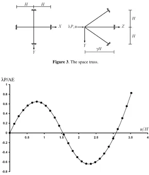
In this section, some examples are given to evaluate the advantages and disadvantages of the suggested methods. The behavior of the provided structures is highly non-linear (including snap-through and snap-back behaviors) and the analyses have been performed by several incremental factors. By doing this, the effects of incremental parameters on the iterative process can be seen. In the following, four space trusses and a shallow arch are analyzed by the cylindrical arc-length and five suggested methods. In these examples, the effect of material non-linearity is not considered and this paper focuses on geometrically non-linear structures. Each example contains the shape and properties of the structure, load-displacement diagram and a table. Tables give the number of iteration for each method which is related to the incremental factor. The sign of "—" in tables shows that the approach becomes divergent. In addition, the diagrams of load-displacement are based on cylindrical arc-length with displacement increment.

(6)

1

A= , E=100, H=100, γ= 2.375, P=100,

2 . 0

1

1=

λ

∆ , JD=2, Jmax=10 and permitted error 4

C=10−

ε .

The equilibrium path of the structure includes two limit points (Figure 4). Table 1 reveals that all the suggested techniques have the same iteration number in comparison with the cylindrical

arc-lengthmethod foreach increment factor.As Table1 shows,loadparametermakesthe analysisdivergent.

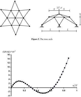
5.2. The Truss Arch As it can be seen, Figure 5 shows a truss arch with 24 members and 21 degrees of freedom [23,18].

In this figure, the values of A, E, H, L, S and

W are equal to 317 mm2, 3 × 103 N/mm2, 62.16 mm,

Figure 3. The space truss.

λP/AE

Figure 4. The load-displacement diagram for the space truss.

TABLE 1. The Number of Iterations in the Analysis of the Space Truss.

Method Incremental Factors

Load Displacement Length Perimeter Area

(7)

433 mm, 250 mm and 20 mm, respectively. At the beginning of analysis, P is assumed 150N, 1

1

λ

∆ is

5 .

0 , J_Dequals5,J_maxis 15andε_Cis equal to ₁₀−4_.

Figure 6 illustrates the load-displacement diagram containing two limit points. Table 2 presents the number of iteration for each approach with several incremental parameters. As it is shown, the displacement factor has almost the least iteration during analysis. Again, the load parameter does not obtain the correct equilibrium path. In this example, Minimizing Residual Length and Minimizing Residual Perimeter converge to the equilibrium point for most of the incremental factors, although the number of iteration has increased.

5.3.The Truss Dome The space truss in Figure7 has 264 members and 219 degrees of freedom [24]. This structure includes many degrees of freedom. Some characteristics of this truss are: A = 450 mm2, E = 2.1 × 105 N/mm2, H = 4580 mm, P = 15 × 103 N,

15 . 0

1

1=

λ

∆ , JD=5, Jmax=20 and

4

C=10−

ε .

The load-displacement diagram, similar to previous examples, contains two limit points (Figure 8). The number of iterations for each method is provided in Table 3. As it can be observed, the displacement factor leads to answer for all mentioned techniques, especially for Cylindrical Arc-Length and Minimizing Residual Area which reach the minimum iteration.

Four suggested methods converge to the equilibrium path with three different incremental factors in similar way.

5.4. The Shallow Truss Dome The structure in Figure 9 has 168 members and 147 degrees of freedom [25,18]. Some characteristics of the shallow truss dome are assumed as follows: A = 100 mm2, E = 103 N/mm2, H = 1790.22 mm, P = 1000 N,

25 . 0

1

1=

λ

∆ , JD=6, Jmax=20 and εC=10−4.

Figure 10 illustrates the diagram of the load-displacement. This structure buckles two times during analysis. Table 4 presents the number of iteration for each approach with several incremental factors. Except Minimizing Residual Area method, all techniques trace the equilibrium path with displacement, length and perimeter increments. Cylindrical Arc-Length and Orthogonality of n

1

u

∆

and n i

u

δ reach the equilibrium path with minimum iteration. Conversely, Linearization of Arc-Length needs the maximum iteration.

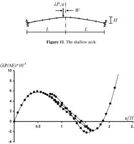
5.5. The Shallow Arch The structure shown in Figure 11 has a complicated behavior [6]. The arch is located on a circle arc and divided into 10 elements. The values of A, I, E, H, L and W

are dimensionless and equal to ₁₀4_, ₁₀8_, ₂₀₀_,

500, 5000 and 200, respectively. At the beginning of analysis, P is 1000, ∆λ11 is assumed 0.4, JD

equals 5, Jmax is 15 and εC is equal to 4

10− . The equilibrium path of the structure includes two turning points and two limit points. Figure 12 displays the diagrams ofload-displacement.Table5 presents the number of iteration for each technique with several incremental parameters. As it can be seen, the Orthogonality of n

1

u

∆ and n

i

u

δ and Minimizing Residual Area are become divergent for all incremental factors. On the other hand, Cylindrical Arc-Length with length incremental factor results in the minimum iteration. Linearization of Arc-Length, Minimizing Residual Length and Minimizing Residual Perimeter act similarly. It is noteworthy that these methods are convergence for a load incremental factor.

6. CONCLUSION

(8)

Figure 5. The truss arch.

(λP/AE)*10-4

Figure 6. The load-displacement diagram for the truss arch.

TABLE 2. The Number of Iterations in the Analysis of the Truss Arch.

Method

Incremental Factors

Cylindrical Arc-Length Linearization of Arc-Length

Orthogonality of n 1

u

∆ and n

i

u

δ

Minimizing the Residual Length Minimizing the Residual Area

Minimizing the Residual Perimeter

— —

61 61

61 153

66 145

— —

— 96

69 74

69 100

92 100

— —

— 102

(9)

Figure 7. The truss dome.

(λP/AE)*10-5

Figure 8. The load-displacement diagram for the truss dome.

TABLE 3. The Number of Iterations in the Analysis of the Truss Dome.

Method

Incremental Factors

u

∆ and n

i

u

δ

Minimizing the Residual Length

Minimizing the Residual Area Minimizing the Residual Perimeter

— —

52 74

69 75

52 79

— 65

93 69

— 69

— 64

93 69

— 69

— —

(10)

Figure 9. The shallow truss dome.

(λP/AE)*10-3

Figure 10. The load-displacement diagram for the shallow truss dome.

TABLE 4. The Number of Iterations in the Analysis of the Shallow Truss Dome.

Method

Incremental Factors

Cylindrical Arc-Length

Linearization of Arc-Length

Orthogonality of ∆u1n and n i

u

δ

Minimizing the Residual Length

Minimizing the Residual Area

—

99

244

101

116

—

116

140

195

147

183

—

183

152

193

141

177

—

176

—

(11)

7. REFERENCES

1. Batoz, J.L. and Dhatt, G., “Incremental Displacement Algorithms for Nonlinear Problems”, Int. J. Numer. Meth. Engng., Vol. 14, (1979), 1262-1266.

2. Chen, H. and Blandford, G.E., “Work-Increment-Control Method for Non-Linear Analysis”, Int. J. Numer. Meth. Engng., Vol. 36, (1993), 909-930. 3. Lin, T.W., Yang, Y.B. and Shiau, H.T., “A Work Weighted

State Vector Control Method for Geometrically

Figure 11. The shallow arch.

(λP/AE)*10-4

Figure 12. The load-displacement diagram for the shallow arch.

TABLE 5. The Number of Iterations in the Analysis of the Shallow Arch.

Method

Incremental Factors

u

∆ and n

i

u

δ

Minimizing the Residual Length Minimizing the Residual Area

—

566 —

270 —

246

240

319 —

274 —

289

165

340 —

290 —

268

—

385 —

— —

—

378

— —

591 —

(12)

Nonlinear Analysis”, Comput. Struct., Vol. 46, (1993), 689-694.

4. Widjaja, B.R., “Path-Following Technique Based on Residual Energy Suppression for Nonlinear Finite Element Analysis”, Comput. Struct., Vol. 66, (1998), 201-209.

5. For de, B.W.R. and Stiemer, S.F., “Improved Arc Length Orthogonality Methods for Nonlinear Finite Element Analysis”, Comput. Struct., Vol. 27, (1987), 625-630.

6. Clarke, M.J. and Hancock, G.J., “A Study of Incremental-Iterative Strategies for Non-Linear Analyses”, Int.J.Numer.Meth.Engng.,Vol.29,(1990),1365-1391. 7. Regon, S.A., Gurdal, Z. and Watson, L.T., “ A

Comparison of Three Algorithms for Tracing Nonlinear Equilibrium Paths of Structural Systems”, Int. J. Solid Struct., Vol. 39, (2002), 689-698.

8. Riks, E., “An Incremental Approach to the Solution of Snapping and Buckling Problems”, Int. J. Solid Struct., Vol. 15, (1979), 529-551.

9. Crisfield, M.A., “A Fast Incremental/Iterative Solution Procedure that Handles Snap-Through”, Comput. Struct., Vol. 13, (1981), 55-62.

10. Bashir-Ahmed, M. and Xiao-Zu, S., “Arc-Length Technique for Nonlinear Finite Element Analysis”, J. Zhejiang Univ. SCI, Vol. 5, No. 5, (2004), 618-628. 11. Fujii, F. and Ramm, E., “Computational Bifurcation

Theory: Path-Tracing, Pinpointing and Path-Switching”, Engng. Struct., Vol. 19, No. 5, (1997), 385-392. 12. Kouhia, R. and Mikkola, M., “Tracing the Equilibrium

Path Beyond Simple Critical Points”, Int. J. Numer. Meth. Engng., Vol. 28, (1989), 2923-2941.

13. Yang, Y.B., Lin, S.P. and Leu, L.J., “Solution Strategy and Rigid Element for Nonlinear Analysis of Elastically Structures Based on Updated Lagrangian Formulation”, Engng. Struct., Vol. 29, (2007), 1189-1200.

14. Lopez,S.,“An Effective Parametrization for Asymptotic Extrapolations”, Comput. Meth. Appl. Mech. Engng.,

Vol. 189, (2000), 297-311.

15. Lopez, S., “Geometrically Nonlinear Analysis of Plates and Cylindrical Shells by a Predictor-Corrector Method”, Comput. Struct., Vol. 79, (2001), 1405-1415. 16. Kim, J.H. and Kim, Y.H., “A Predictor-Corrector Method

for Structural Nonlinear Analysis”, Comput. Meth. Appl. Mech. Engng., Vol. 191, (2001), 959-974. 17. Mallardo, V.and Alessanderi, C., “Arc-Length Procedures

with BEM in Physically Nonlinear Problems”, Engng. Anal. Bound. Elem., Vol. 28, (2004), 547-559. 18. Saffari, H., Fadaee, M.J. and Tabatabaei, R., “Nonlinear

Analysis of Space Trusses using Modified Normal Flow Algorithm”, ASCE J. Struct. Engng., Vol. 134, No. 6, (2008), 998-1005.

19. Bathe, K.J. and Dvorkin, E.N., “On the Automatic Solution of Non-Linear Finite Element Equations”, Comput. Struct., Vol. 17, (1983), 871-879.

20. Rezaee Pajand, M. and Taghavian Hakkak, M., “Nonlinear Analysis of Truss Structures using Dynamic Relaxation”, International Journal of Engineering, Vol. 19, No. 1B, (December 2006), 11-22.

21. Legaro, S.S. and Valvo, P.S., “Large Displacement Analysis of Elastic Pyramidal Trusses”, Int. J. Solid Struct., Vol. 43, No. 16, (2004), 4867-4887.

22. Casciaro, R., Salerno, G. and Lanzo, A.D., “Finite Element Asymptotic Analysis of Slender Elastic Structures: A Simple Approach”, Int. J. Numer. Meth. Engng., Vol. 35, (1992), 1397-1426.

23. Krenk, S., “An Orthogonal Residual Procedure for Non-Linear Finite Element Equations”, Int. J. Numer. Meth. Engng., Vol. 38, (1995), 823-839.

24. Krishnamoorthy, C.S., Ramesh, G. and Dinesh, K.U., “Post-Buckling Analysis of Structures by Three-Parameter Constrained Solution Techniques”, Finit. Elem. Anal. Design, Vol. 22, (1996), 109-142. 25. Powell, G. and Simons, J., “Improved Iteration Strategy