ORIGINAL ARTICLE
Optimization of Uncertain Structures
with Interval Parameters Considering Objective
and Feasibility Robustness
Jin Cheng
1, Zhen‑Yu Liu
2*, Jian‑Rong Tan
1, Yang‑Yan Zhang
1,3, Ming‑Yang Tang
1and Gui‑Fang Duan
1,2,3Abstract
For the purpose of improving the mechanical performance indices of uncertain structures with interval parameters and ensure their robustness when fluctuating under interval parameters, a constrained interval robust optimization model is constructed with both the center and halfwidth of the most important mechanical performance index described as objective functions and the other requirements on the mechanical performance indices described as constraint functions. To locate the optimal solution of objective and feasibility robustness, a new concept of interval violation vector and its calculation formulae corresponding to different constraint functions are proposed. The math‑ ematical formulae for calculating the feasibility and objective robustness indices and the robustness‑based preferen‑ tial guidelines are proposed for directly ranking various design vectors, which is realized by an algorithm integrating Kriging and nested genetic algorithm. The validity of the proposed method and its superiority to present interval optimization approaches are demonstrated by a numerical example. The robust optimization of the upper beam in a high‑speed press with interval material properties demonstrated the applicability and effectiveness of the proposed method in engineering.
Keywords: Robust optimization, Uncertain structure, Interval violation vector, Feasibility robustness, Objective robustness, Nested genetic algorithm
© The Author(s) 2018. This article is distributed under the terms of the Creative Commons Attribution 4.0 International License (http://creativecommons.org/licenses/by/4.0/), which permits unrestricted use, distribution, and reproduction in any medium, provided you give appropriate credit to the original author(s) and the source, provide a link to the Creative Commons license, and indicate if changes were made.
1 Introduction
The uncertainties in material properties, geometric dimensions, load conditions and so on are ubiquitous for engineering structures [1]. The optimal solutions to the optimization models of engineering structures that neglect these uncertainties may be infeasible because their mechanical performance indices will fluctuate under the uncertainties [2]. Hence these uncertainties must be considered in handling the optimization prob-lems of uncertain engineering structures [3, 4]. Robust design optimization is a frequently-utilized methodol-ogy to improve the robustness of structures and reducing the sensitivities of their mechanical performance indices to uncertain factors [5–8]. In the construction of various
robust optimization models, the objective robustness is often achieved by simultaneously optimizing the mean of the objective mechanical performance index and minimizing its variation under uncertainties while the constraint robustness is to ensure the satisfaction of con-straints when the constraint performance indices fluctu-ate under the influences of uncertain parameters [9].
Most researches on robust design optimization were conducted based on the assumption that the probabil-istic distributions of uncertain factors were known [10,
11]. For instance, Doltsinis et al. [12] applied the pertur-bation technique and the incremental loading procedure for the response analysis of path-dependent non-linear structural systems with random parameters, and evalu-ated the sensitivities of the mean and variance of the structural performance function by direct differentiation in the framework of stochastic finite element analysis.
Tang and Périaux [13] proposed a robust optimization
method capable of locating Pareto and Nash equilibrium
Open Access
*Correspondence: [email protected]
2 State Key Laboratory of CAD & CG, Zhejiang University, Hangzhou 310027, China
solutions. Zhao and Wang [14] proposed an efficient approach for solving the robust topology optimization problem of structures under loading uncertainty based on linear elastic theory and orthogonal diagonalization of symmetric matrices. Sahali et al. [15] proposed an effi-cient genetic algorithm (GA) for multi–objective robust optimization of machining parameters considering ran-dom uncertainties. Martínez–Frutos et al. [16] proposed a robust shape optimization approach of continuous structures via the level set method, which modeled the uncertainty in loads and material as random variables with different probability distributions as well as random fields. However, it is often difficult or computationally expensive to determine the probabilistic distributions of uncertain factors in many engineering problems [17].
In order to realize the robust optimization of uncertain structures in the absence of the probabilistic distribution information of uncertainties, several non-probabilistic methods have been proposed in recent years to account for the uncertainties [18, 19]. Au et al. [20] proposed a robust design method based on the convex model and achieved the robustness of the objective function by minimizing the worst value of unsatisfactory degree functions of the uncertain parameters and ensured the feasibility robustness by a sub-optimization conducting
the worst-case analysis. Takewaki and Ben–Haim [21]
represented the uncertainties in the power spectral den-sity of load and the parameters of the structure’s vibration model by info-gap models, and proposed a robust—sat-isficing methodology for the info-gap robust design of uncertain structures. However, the above methods are very complex when the parameter numbers are large. Sun et al. [22] proposed a bi-level mathematical model with interval objective and constraint functions for robust design optimization. The single objective function was converted into two objective functions for minimizing the mean and variation while the constraint functions were reformulated with the acceptable robustness level. However, the so-called robust solution obtained by their method cannot ensure the robustness of all constraints. Karer and Skrjanc [23] proposed a robust optimization framework for PID controllers by describing the uncer-tain dynamics of the process as an interval model, which was firstly transformed into a deterministic model and then solved by a particle swarm optimization algorithm. Li et al. [24] proposed an actuator placement robust optimization method for active vibration control system with interval parameters. Both nominal value and radius of the performance index were considered in the inter-val optimization model, which was also transformed into a deterministic one by weighted processing and then solved by GA.
To sum up, present non-probabilistic robust optimiza-tion approaches have difficulties in ensuring the robust-ness of all constraints and achieving the globally optimal robust solutions to real engineering problems. Moreover, the solution algorithms employed in the present robust optimization approaches based on interval models are indirect ones. That is, they firstly transformed the inter-val models into deterministic ones and then solved the resulting deterministic models by conventional deter-ministic optimization algorithms. The shortcomings of such indirect robust optimization approaches are similar to the indirect ones for solving general interval optimi-zation models [25, 26]. Specifically, different acceptable robustness levels or satisfactory degrees of interval con-straints prescribed in model transform process will lead to different optimal solutions. Additionally, the trans-formation of interval models into deterministic ones also deviates from the original intention of uncertainty modeling.
To avoid the limitations of indirect algorithms for solv-ing interval optimization models, we have proposed a direct interval optimization algorithm for uncertain structures by introducing the concept of the degree of interval constraint violation (DICV) [27] based on Hu’s “center first halfwidth next” interval order rela-tion [28]. Specifically, a design vector x has zero DICV for constraint g(x,U)≤B= [bL,bR] =
bC,bW
when
gC(x) <bC or gC(x)=bC and gW(x)≤bW; otherwise,
the DICV is nonzero for the constraint (where g(x,U) is
the mechanical performance index of a structure under the influence of interval parameter U, B is the given interval constant, superscripts L, R, C, W indicate the left bound, right bound, center and halfwidth of an interval). The feasibility of a design vector x is determined by the total DICV of all its interval constraints and a design vec-tor x is regarded as feasible when its total DICV is zero. And finally the design vectors are directly sorted accord-ing to the DICV–based preferential guidelines. How-ever, there may be gL(x)≤bL or/and gR(x)≥bR when gC(x)≤bC. That is, the constraint g(x,U)≤B may be
violated although design vector x is regarded as feasible when gC(x)≤bC according to the definition of DICV.
Consequently, the DICV–based direct interval optimiza-tion algorithm cannot ensure the constraint robustness of the optimal solution.
mechanical performance index in a constraint function. The mathematical formulae for calculating the interval violation vectors of a design vector corresponding to var-ious constraint functions are provided. Then the objec-tive and feasibility robustness indices of various design vectors can be calculated based on their values of total interval violation vectors. And finally, the design vec-tors of an uncertain structure are sorted according to the robustness-based preferential guidelines, which is real-ized by integrating the Kriging technique and nested GA.
2 Robust Optimization Model of an Uncertain Structure with Interval Parameters
The mechanical performance indices of an uncertain structure are described as the functions of both design variables and interval parameters. The center and halfwidth of the most important mechanical perfor-mance index of the uncertain structure are described as the objective functions while the requirements on the other mechanical performance indices are described as constraint functions. Then the robust optimization model of an uncertain structure with interval parameters is described as
where
s.t.,
where x is an n-dimensional design vector, U is a
q-dimensional interval parameter vector;f(x,U) is the
most important performance index while gi(x,U) is the ith performance index with restriction. Both f(x,U) and
gi(x,U) are nonlinear continuous functions about x and U, but the mechanical performance indices gi(x,U) in
constraints may degenerate into deterministic ones, such as gi(x). fC(x) and fW(x) are the center and halfwidth of f(x,U) while fL(x) and fR(x) are the left and right
(1)
min
x
fC(x),fW(x),
fC(x)=fR(x)+fL(x)2
=
max U
f(x,U)+min U
f(x,U)
2;
fW(x)=
fR(x)−fL(x)
2 = max U
f(x,U)−min U
f(x,U)
2.
gi(x,U)≤(≥)Bi=bLi,bRi,i=1, 2,· · ·,p; x=(x1,x2,· · ·,xn);
U =
U1,U2,· · · ,Uq;
Uj=
uLj,uRj,j=1, 2,· · · ,q.
bounds of f(x,U). B
i is the given interval constant for the
ith constraint, which may degenerate into a real number. The left and right bounds of the mechanical perfor-mance index gi(x,U) in the ith interval constraint func-tion of Eq. (1) can be computed by
where p is the number of constraint functions.
3 Definition of the Interval Violation Vector and its Calculation
3.1 Definition of the Interval Violation Vector for an Interval Constraint
For the ith interval constraint gi(x,U)≤Bi= [bLi,bRi]
in Eq. (1), there are a total of six positional relations between gi(x,U)= [giL(x),giR(x)] and Bi = [bLi,bRi] as
shown in Figure 1. It is obvious that the interval con-straint gi(x,U)≤Bi = [bLi,bRi] is fully satisfied when the
positional relation of the mechanical performance index
gi(x,U) and the given interval constant Bi is illustrated
as Figure 1(a) when bLi −giL(x)≥gR
i (x)−giL(x) and bRi −giR(x)≥bR
i −bLi, including the case that giR(x)=bLi . Correspondingly, the violation degrees for both the left and right bounds of the interval mechanical performance index gi(x,U) are zero in the case shown in Figure 1(a).
Therefore, the following concept of interval violation vector is introduced to describe the violation degree of a design vector for an interval constraint.
Definition 1 (Interval violation vector)
The interval violation vector of an interval constraint gi(x,U)≤Bi= [bLi,bRi] is a two-dimensional vector, the
components of which describe the violation degrees of the left and right bounds of the interval mechanical per-formance index gi(x,U) of an uncertain structure under
the influence of interval parameter vector U.
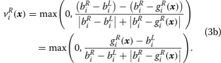
Specifically, the interval violation vector of constraint gi(x,U)≤Bi= [bLi,bRi] is
where viL(x) and viR(x) are the violation degrees of the left
and right bounds of gi(x,U), and there is
(2)
giL(x)=min
U gi(
x,U); giR(x)=max
U gi(
x,U); i=1, 2,· · ·,p,
(3)
vi(x)=
vLi(x),vRi(x)
,
(3a)
viL(x)=max
0,
giR(x)−giL(x)−bLi −giL(x)
giR(x)−giL(x) +
bLi −giL(x) =max 0, g R
i (x)−bLi giR(x)−gL
i(x)+
bLi −giL(x)
As can be seen from Eq. (3), the interval violation vector vi(x)=
vLi(x),vRi(x) of interval constraint
gi(x,U)≤Bi= [bLi,bRi] has the following properties:
(1) There are 0≤viL(x)≤1 and 0≤vR
i(x)≤1 for any
design vector x.
(2) There is vi(x)=(0, 0) when giR(x)≤b L
i as shown in Figure 1(a).
(3) There is vLi(x)=1 when gL i(x)≥b
L
i, see
Fig-ures 1(d)–(f).
(4) There is viR(x)=1 when gR
i (x)≥b
R
i, see Figures 1(c),
(e), (f).
3.2 Calculation of the Interval Violation Vector for Various Constraints
For a mechanical performance index independent of interval parameters, there is gi(x)=giL(x)=g
R
i(x), and
the constraint gi(x,U)≤Bi= [bLi,bRi] in Eq. (1)
degen-erates as gi(x)≤Bi= [bLi,bRi] correspondingly. Then the
(3b)
vRi(x)=max
0,
bRi −bLi
−bRi −giR(x)
biR−bLi +
bRi −giR(x)
=max
0, g
R
i (x)−bLi bRi −bLi +bRi −giR(x)
.
formula for calculating the interval violation vector of such a constraint should be adjusted as Eq. (4).
In engineering, the interval constant Bi= [bLi,bRi]
in Eq. (1) may also degenerate into a real number,
namely, there is bi=bLi =bRi. In this case, the con-straint gi(x,U)≤Bi= [biL,bRi] in Eq. (1) degenerates as
gi(x,U)≤bi and the formula for calculating the interval
violation vector of such a constraint should be adjusted as Eq. (5).
Furthermore, the constraint gi(x,U)≤Bi= [bLi,bRi]in
Eq. (1) will degenerate as gi(x)≤bi when the mechanical
performance index is independent of the interval param-eters and the interval constant degenerates into a real number. And then the formula for calculating the interval violation vector for such a constraint will be simplified as Eq. (6).
As can be observed from Eqs. (3)–(6), there are
vi(x)=(0, 0) when gi(x)=bLi or bi=giR(x) or gi(x)=bi ,
otherwise, the values of vi(x) can be calculated by Eq. (3).
Consequently, the formula for calculating the interval violation vector of constraint gi(x,U)≤Bi= [bLi,biR] can
be concluded as Eq. (7).
Similarly, the formula for calculating the interval viola-tion vector of constraint gi(x,U)≥Bi= [bLi,bRi] can be
deduced as Eq. (8), the detailed derivation of which is not provided here for space–saving sake.
(4)
vi(x)=
� max �
0, gi(x)−bLi � �bLi−gi(x)
� �
� , max
�
0, gi(x)−bLi bRi−bLi+
� � �b
R i−gi(x)
� � �
��
, when gi(x)�=bLi;
(0, 0), when gi(x)=bLi.
(5)
vi(x)= � max � 0, g R i(x)−bi
giR(x)−giL(x)+
� �bi−giL(x)
� � � , max � 0, g R i(x)−bi
� � �bi−g
R i(x)
� � �
��
, when bi �=giR(x);
(0, 0), when bi=giR(x).
(6)
vi(x)= max
0, gi(x)−bi
|bi−gi(x)|
, max0, gi(x)−bi
|bi−gi(x)|
, when gi(x)�=bi;
(0, 0), when gi(x)=bi.
(7)
vi(x)=
(0, 0), when sign�� � �
giL(x)−gR i (x)
�
×�bLi −bRi�� � �
+sign��
�giR(x)−bLi � � �
=0;
�
max
�
0, giR(x)−bLi gR
i(x)−giL(x)+ � �bL
i−giL(x) � �
�
, max
�
0, giR(x)−bLi bRi−biL+
� � �b
R i−giR(x)
� � � �� , otherwise. (8)
vi(x)=
(0, 0), when sign�� � �
bLi −bRi�
×�giL(x)−gR
i (x) ��
� �
+sign��
�bRi −giL(x) � � �
=0;
�
max
�
0, bRi−giL(x)
bR i−bLi+
� �gL
i(x)−bLi
� � �
, max
�
0, bRi−giL(x)
giR(x)−giL(x)+
� � �g
R i(x)−bRi
� � �
��
, otherwise.
Then design vector x is regarded as feasible robust when vT(x)=(0, 0) and it is not when vT(x) > (0, 0) .
And the feasibility robustness index of design vector x can be calculated by
As can be seen from Eq. (10), the larger total interval violation vector will lead to the smaller feasibility robust-ness index for a design vector. Moreover, the feasibility robustness index for a design vector has the following properties.
(1) For a feasible robust design vector x, there is IFR(x)=1.
(2) For a design vector x that is not feasible robust, there is 0≤IFR(x) <1.
(3) The larger feasibility robustness index indicates the better acceptability of a design vector as far as the constraints are concerned.
4.2 Objective Robustness Index and its Calculation
The center and halfwidth of the objective mechanical performance index should be regarded as equally impor-tant in the robust optimization of an uncertain structure
(10)
IFR(x)=1− |vT(x)|
√ 2p=
1−
vLT(x)2+vRT(x)2
√
2p. 4 Preferential Guidelines Considering Objective
and Feasibility Robustness
In order to directly solve the robust optimization model in Eq. (1), two robustness indices are introduced to eval-uate the objective and feasibility robustness of a design vector. The feasibility robustness index is utilized to evaluate the acceptability of a design vector as far as the constraint functions are concerned while the objective robustness index is utilized to evaluate the superiority and robustness of a design vector as far as the objective mechanical performance index is concerned. Then the robustness–based preferential guidelines are proposed for realizing the direct ranking of various design vectors.
4.1 Feasibility Robustness Index and its Calculation
The feasibility robustness index can be calculated from the total interval violation vector of all the constraints in the robust optimization model considering that the total interval violation vector reversely reflects the feasibility robustness of a constraint function. Specifically, the total interval violation vector corresponding to design vector x can be calculated by Eq. (9) as far as the interval violation vectors of all constraints gi(x,U)≤(≥)Bi(i=1, 2,· · ·,p)
are calculated by Eq. (7) or Eq. (8):
(9)
vT(x)=
p
i=1
regardless of their possible difference in orders of mag-nitude. To achieve this aim, all the feasible robust design vectors are sorted according to their corresponding val-ues of fC(x) and fW(x) with the rank numbers obtained
as rC(x), rW(x) respectively. A design vector with the
smaller objective value is assigned a larger rank number and the design vector with the largest objective value is assigned the rank number of 1. Then the rank vector of design vector x are generated as r(x)=
rC(x),rW(x)
. And finally, the objective robustness index of design vec-tor x is calculated by
It is obvious from Eq. (11) that the objective robust-ness index is positive for any design vector, and the larger objective robustness index indicates the better and more robust of a design vector as far as the objective mechani-cal performance index is concerned.
4.3 Preferential Guidelines for Ranking Various Design Vectors
As far as their objective and feasibility robustness indices are calculated by Eq. (10) and Eq. (11), all of the alterna-tive design vectors can be ranked according to the follow-ing preferential guidelines:
(1) A feasible robust design vector is always superior to an infeasible one. That is, design vector x1 is superior to design vector x2 when IFR(x1)=1 and IFR(x2) <1 .
(2) The infeasible design vectors are ranked accord-ing to their correspondaccord-ing values of feasibility robustness indices. Specifically, infeasible design vector x1 is superior to infeasible design vector x2
when IFR(x1) >IFR(x2).
(3) The feasible robust design vectors are ranked according to their objective robustness indi-ces. Specifically, feasible design vector x1 is superior to feasible design vector x2 when IOR(x1) >IOR(x2).
5 Integrated Algorithm for Directly Solving the Interval Robust Optimization Model
A robust optimization algorithm integrating Kriging models and nested GA is proposed to directly solve the constrained interval robust optimization model of the uncertain structure. The Kriging model is utilized here to replace finite element analysis (FEA) for efficiently computing the mechanical performance indices of the uncertain structure. For the mechanical performance index influenced by n-dimensional design vector x and
q-dimensional interval vector U, such as f(x,U) and
(11)
IOR(x)=
rC(x)2
+rW(x)2 .
gi(x,U) in Eq. (1) is concerned, the sample points for
constructing the Kriging model should be generated in
the (n+q)-dimensional space determined by n design
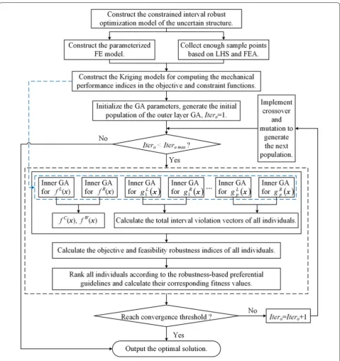
variables and q interval parameters based on Latin hyper-cube sampling (LHS). To ensure the prediction accuracy of Kriging models, the adaptive resampling technology proposed in our previous work [29] is also adopted. Spe-cifically, the construction of every Kriging model is an iterative process until the achievement of satisfactory local and global precision evaluated by multiple correla-tion coefficient R2 and relative maximum absolute error (RMAE). The inner layer GAs integrated with Kriging models calculate in parallel the intervals of the mechani-cal performance indices under the influence of uncer-tain parameters while the outer layer GA realizes the direct sorting of various design vectors according to the robustness-based preferential guidelines and locates the optimal solution to the constrained interval robust opti-mization model.
The flowchart of the proposed direct interval robust opti-mization algorithm is illustrated in Figure 2, the implemen-tation of which proceeds as follows.
Step 1: Construct the robust optimization model of an uncertain structure with interval param-eters. The mechanical performance indices of the uncertain structure are described as the functions of design variables and inter-val parameters. The center and halfwidth of the most important mechanical performance index are described as objective functions while the requirements of the other mechani-cal performance indices are described as con-straint functions.
Step 2: Construct the Kriging models for efficiently computing the mechanical performance indi-ces of the uncertain structure based on finite element (FE) model, LHS and adaptive resam-ple technology.
Step 3: Initialize the GA parameters involved in the nested optimization, including the population sizes, maximum iteration numbers, crossover and mutation probabilities of the inner and outer layer GAs. Set the iteration number of the outer layer GA as 1 and generate the initial population.
implemented in parallel for computing the left and right bounds of the mechanical perfor-mance indices.
Step 5: Output the design vector with the largest fit-ness value if the convergent threshold or maxi-mum iteration number of the outer layer GA is reached. Otherwise, increase the iteration num-ber of the outer layer GA by 1 and go to Step 4.
6 Illustrative Examples
Two illustrative examples are investigated in this section to verify the effectiveness of the proposed approach for directly solving interval robust optimization problems and its applicability in engineering practice. The con-struction of Kriging models is unnecessary for the first example since its objective and constraint functions are analytical. It is obvious that the proposed robust interval
optimization algorithm has the same advantages as our previous one in realizing the direct solution of interval optimization problems and avoiding the complicated model transformation process. Consequently, the opti-mization results obtained by the proposed algorithm are only compared with those obtained by the direct one hereinafter.
6.1 Numerical Example
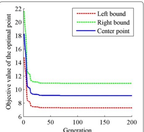
The constrained interval robust optimization model in Eq. (12) is utilized as a benchmark example, which is firstly solved by the proposed algorithm with the GA parameters listed in Table 1. Besides the maximum itera-tion number given as a stop criterion, the outer layer GA evolution is terminated when the absolute difference of
fC(x) between the optimal solution and the average of
current population is less than 10−3.
Figure 3 illustrates the convergent curves of numeri-cal example obtained by the proposed algorithm. The objective value of the optimal solution con-verges at the 78th generation. The optimal solution is
xo=(3.17, 0.02, 2.00), the corresponding objectives and
constraints of which are fC(xo)=9.11, fW(xo)=1.80, g1(xo, U)= [10.00, 12.41] andg2(xo, U)= [7.55, 9.94] respectively. It is obvious that both constraints in Eq. (12) are fully satisfied at xo=(3.17, 0.02, 2.00),
demonstrat-ing the feasibility robustness of two constraints.
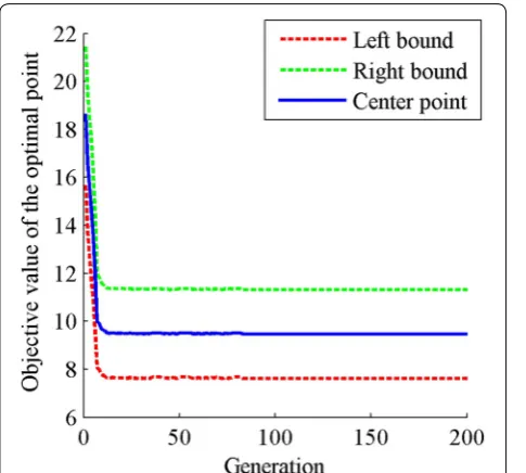
The robust optimization model in Eq. (12) is also solved by our previous algorithm [27] with the GA parameters and convergent threshold prescribed the same as those in the proposed one. The objective values of the opti-mal solution converge at the 86th generation, with the
(12)
min
x �
fC(x),fW(x)� =
min
x ��
fR(x)+fL(x)��
2,�
fR(x)−fL(x)��
2�
wherefR(x)=max
U f(
x,U),fL(x)=min
U f(
x,U);
f(x,U)=U12(x1+2)+U2x22+U32x23 s.t.,
g1(x,U)=U1x21−U22x2+U3x3≥ [8.0, 10.0];
g2(x,U)=U1x1+U2x2+U32x23+1.0≥ [4.5, 5.0].
x1∈ [1, 10],x2∈ [0, 9],x3∈ [2, 8].
U1=[0.8, 1.0],U2=[0.9, 1.1],U3=[1.0, 1.2].
optimal solution obtained as x∗=(3.11, 0.20, 2.08) and
the convergent curves illustrated in Figure 4.
Table 2 lists the optimization results of the numerical example obtained by two algorithms. As can be seen from Table 2, the 2nd constraint function g2(x,U)≥ [4.5, 5.0]
is fully satisfied at both the optimal solutions. But the 1st constraint function g1(x,U)≥ [8.0, 10.0] may be violated at the optimal solution x∗=(3.11, 0.20, 2.08) obtained by our previous algorithm while it is always satisfied at the optimal solution xo=(3.17, 0.02, 2.00) obtained by
the proposed algorithm. That is, the optimal solution x* obtained by our previous algorithm is not a robust one as far as the constraints are concerned while the opti-mal solution xo obtained by the proposed algorithm is. The improvement is gained from the definition of inter-val violation vector and the robustness-based prefer-ential guidelines. Specifically, the interval constraint
g1(x,U)≥ [8.0, 10.0] at x* is regarded as feasible accord-ing to the “center first halfwidth next” interval order rela-tion for evaluating the feasibility of a constraint in our previous algorithm since g1C(x∗)=10.79>9.0 but x* is
obviously not feasible robust according to the definition of interval violation vector in Section 3. Consequently, the proposed algorithm can yield a more robust solution than our previous one as far as the constraint functions are concerned.
It is also clear from Table 2 that both objective func-tions of the optimal solution obtained by the proposed algorithm are smaller than those obtained by our previ-ous one, which demonstrates that the proposed algo-rithm can obtain a better and more robust solution than
Table 1 GA parameters for numerical example in Eq. (12)
GA Population
size Crossover probability Mutation probability Maximum iteration number
Outer layer 100 0.90 0.05 200 Inner layer 50 0.99 0.05 150
the previous one as far as the objective functions are con-cerned. Moreover, the convergent curves in Figures 3, 4
demonstrate that the proposed algorithm can locate the optimal solution more efficiently than the previous one.
6.2 Engineering Example
The upper beam of an ultra–precision high-speed press is utilized to verify the applicability of the proposed method in the robust optimization of practical engineer-ing structures with interval parameters. Figure 5 illus-trates the 3D solid model and cross section of the upper beam. The geometrical parameters h1, h2, l1, l2, l3 in Fig-ure 5(b) are chosen as design variables while its material density ρ and elastic modulus E are interval parameters.
According to the performance requirements of the upper beam, the maximum deformation reflecting stiff-ness is the most important mechanical performance index, the center and halfwidth of which are described as
the objective functions. With the weight and maximum equivalent stress described as constraint functions, the robust optimization model of the upper beam is con-structed as
where x is the design vector while U is the interval parameter vector; d(x, U) is the maximum deformation;
dC(x) and dW(x) are the center and halfwidth of d(x, U) while dL(x) and dR(x) are the left and right bounds of d(x,
U); w(x, U1) and δ(x, U) are the weight and maximum equivalent stress respectively.
(13)
min
x
dC
(x),dW
(x)
,
wheredC(x)=
dR(x)+dL(x)
2,
dW(x)=
dR(x)−dL(x)
2;
dR(x)=max
U
d(x,U), dL(x)=min U
d(x,U);
s.t.,w(x, U1)=w(x,ρ)≤ [5000, 5010]kg;
δ(x, U)≤ [45, 46]MPa.
x=(h1, h2, l1, l2, l3), U =(U1, U2);
210 mm≤h1≤250 mm, 250 mm≤h2≤300 mm,
80 mm≤l1≤120 mm, 25 mm≤l2≤55 mm,
330 mm≤l3≤390 mm;
U1=ρ= [7280, 7320]kg/m3,
U2=E = [126, 154]GPa.
Figure 4 Convergent curves of numerical example obtained by our previous algorithm
Table 2 The optimization results of numerical example obtained by proposed and previous algorithms
Algorithm Optimal
solution Objective functions Constraint functions [f L, f R],
fC
,fW [g L
1, gR1] [gL2, gR2]
Proposed xo= (3.17,
0.02, 2.00) [7.31,10.92], 9.11, 1.80
[10.00, 12.41] [7.55, 9.94]
Previous x* = (3.11,
0.20, 2.08) [7.62,11.31], 9.47, 1.84
[9.58, 12.00] [7.98, 10.53]
As far as the initial design of the upper beam is con-cerned, there is x = (230, 270, 100, 50, 350) mm. The mechanical performance indices of the initial design under interval parameters E and ρ are listed in Table 3. It is obvious from Table 3 that neither constraint is satisfied for the initial design of the upper beam.
6.2.1 Optimization Results Obtained by Proposed Algorithm
Figure 6 illustrates the 1/4 FE model of the upper beam. A pressure of 800 kN is exerted at every joint between the upper beam and driving oil cylinder. A bearing load of 250 kN is applied on the end bearing hole while a bear-ing load of 500 kN is applied on the mid bearbear-ing hole.
Based on the Kriging models constructed by the adaptive resampling technology with the same preci-sion requirements as Ref. [30] (namely, R2>0.95 and RMAE<0.05), the robust optimization model in Eq. (13) can be directly solved by the proposed algorithm with the GA parameters listed in Table 4. The outer layer GA evolution is terminated when the absolute difference of
dC(x) between the optimal solution and the average of
the current population is less than 10−4.
Table 3 Mechanical performance indices of the initial design scheme of the upper beam
[wL, wR] kg [δL, δR] MPa [d L, d R] mm, dC
,dWmm
[5216.2, 5232.3] [45.21, 50.00] [0.1716, 0.2114], 0.1915, 0.0199
A Fixed Support
B Frictionless Support C Frictionless Support 2 D Force: 8.0x10⁵N
E Bearing Load: 2.5x10⁵N
F Bearing Load 2: 5.0x10⁵N
Figure 6 1/4 FE model of the upper beam: loads and constraints
Table 4 GA parameters for the robust optimization of the upper beam
GA Maximum
iteration number
Population
size Crossover probability Mutation probability
Inner layer 150 60 0.99 0.05 Outer layer 300 120 0.90 0.01
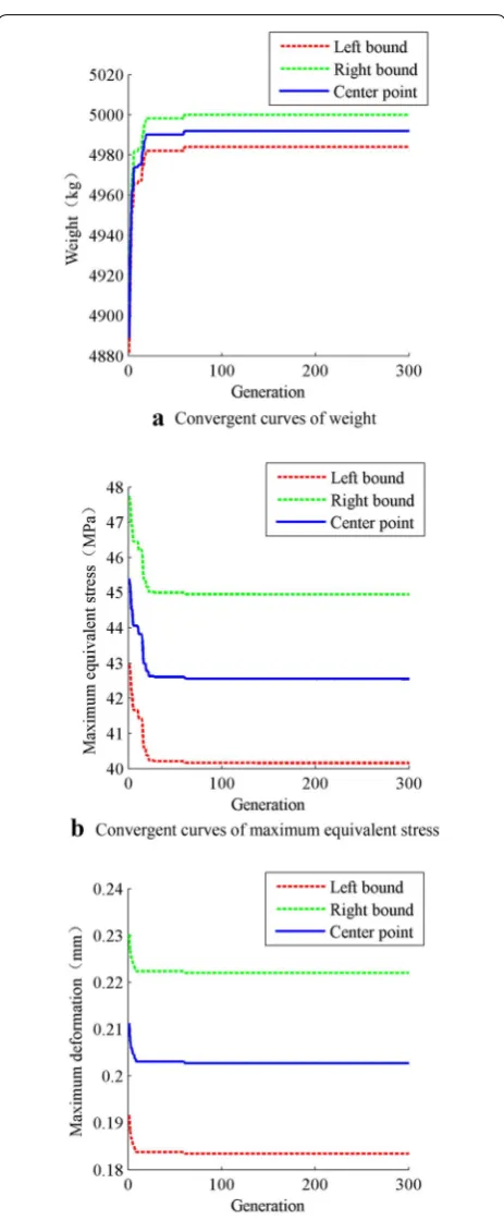
The convergent curves corresponding to the weight, maximum equivalent stress and maximum deforma-tion of the upper beam obtained by the proposed algo-rithm are illustrated in Figure 7, which converge at the 121st generation. The optimal solution is obtained as
xo= (238.89, 280.22, 81.61, 32.73, 386.21), the corre-sponding objective values of which are dC(xo) = 0.2027,
dW(xo) = 0.0193 while the weight and maximum equiva-lent stress in constraints are w(xo, U
1) = [4983.9, 5000.0] and δ(xo, U) = [40.16, 44.95] respectively. It is obvious that both constraints in Eq. (13) are fully satisfied at xo and the feasibility robustness is improved after optimiza-tion. A comparison on the objective values of the optimal solution xo with that of the initial design demonstrates that the objective robustness is also improved since dW is decreased after optimization.
6.2.2 Comparison with Previous Algorithm
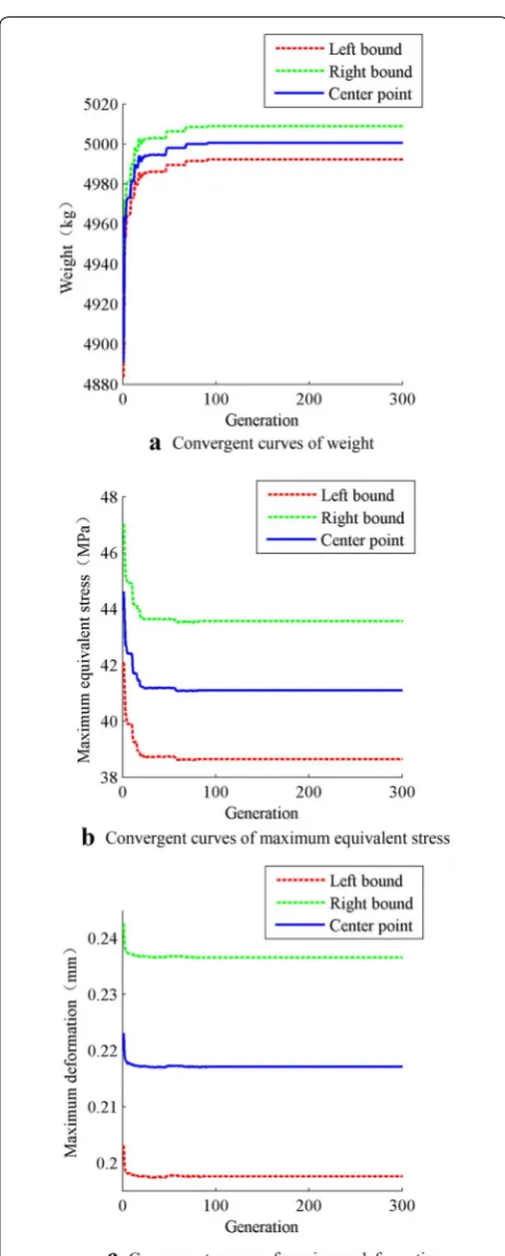
The constrained interval robust optimization model in Eq. (13) is also solved by our previous algorithm [27] with the GA parameters and convergent threshold set-tled the same as those in the proposed algorithm. The objective values of the optimal solution converge at the 146th generation, with the optimal solution obtained as x*= (248.03, 296.28, 85.31, 30.31, 387.89). Figure 8 illustrates the convergent curves of the mechanical per-formance indices of the upper beam obtained by our previous algorithm, a comparison of which with those in Figure 7 demonstrates that the proposed algorithm can locate the optimal solution more efficiently than the pre-vious one.
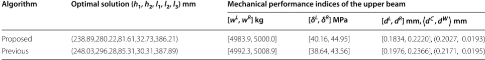
Table 5 compares the optimization results
obtained by the proposed and our previous algo-rithm [27], which shows that the 2nd constraint func-tion δ(x,U)≤ [45, 46]MPa is fully satisfied at both
optimal solutions. But the 1st constraint function w(x,U1)=w(x,ρ)≤ [5000, 5010]kg may be violated
at x*= (248.03, 296.28, 85.31, 30.31, 387.89) obtained by our previous algorithm but it is always satisfied at
xo= (238.89, 280.22, 81.61, 32.73, 386.21) obtained by the proposed algorithm. This is due to the fact that the 1st constraint function is regarded to be satisfied at x* according to the “center first halfwidth next” interval order relation in our previous algorithm since there is w1C(x∗)=5000.6 kg≤5005 kg but its corresponding
interval violation vector is vw(x∗)=(0.26, 0.80)
accord-ing to Definition 1 in Section 3. At the same time, the optimal solution obtained by the proposed algorithm has the smaller center and halfwidth of the maximum defor-mation in the objective functions than those generated by the previous algorithm. Hence the proposed algo-rithm can yield a better and more robust solution than the previous one. This is due to the improved criteria for
evaluating the violation degrees of various constraints and the robustness-based preferential guidelines utilized in the proposed algorithm.
7 Conclusions
To improve the mechanical performance indices of an uncertain structure with interval parameters and ensure their satisfaction with performance requirements when fluctuating under uncertainties, a constrained interval robust optimization model was constructed with both the center and halfwidth of the most important mechani-cal performance index described as objective functions and the other mechanical performance indices included in constraint functions. A novel concept of interval vio-lation vector was proposed for evaluating the feasibility robustness of a design vector, the mathematical formulae for calculating the interval violation vectors of various constraint functions were also provided. Then the robust-ness–based preferential guidelines were proposed for directly ranking various design vectors and an algorithm integrating Kriging technique and nested GA was put forward to realize the direct solution of the constrained interval robust optimization problem.
The proposed direct interval robust optimization algo-rithm has the same advantage as our previous one [27] in avoiding the complex model transformation process from interval to deterministic. The optimization results of the numerical example demonstrated that the pro-posed algorithm was more efficient and effective than our previous one. The robust optimization of the upper beam in a high-speed press with interval material density and elastic modulus demonstrated the feasibility and validity of the proposed method in engineering practice.
Authors’ Contributions
JC, Z‑YL and J‑RT were in charge of the whole trial; JC wrote the manuscript; Y‑YZ, M‑YT and G‑FD assisted with sampling and laboratory analyses. All authors have read and approved the final manuscript.
Author details
1 State Key Laboratory of Fluid Power & Mechatronic Systems, Zhejiang Univer‑ sity, Hangzhou 310027, China. 2 State Key Laboratory of CAD & CG, Zhejiang University, Hangzhou 310027, China. 3 Key Laboratory of Micro‑systems and Micro‑structures Manufacturing of Ministry of Education, Harbin Institute of Technology, Harbin 150001, China.
Authors’ Information
Jin Cheng, born in 1978, is currently an associate professor at State Key Laboratory of Fluid Power & Mechatronic Systems, Zhejiang University, China. She
received her PhD degree from Zhejiang University, China, in 2005. Her research interests include uncertainty modeling, structural optimization and intelligent design. Tel: +86‑571‑87951273; E‑mail: [email protected].
Zhen‑Yu Liu, born in 1974, is currently a professor at State Key Laboratory of CAD & CG, Zhejiang University, China. He received his PhD degree from Zhejiang University, China, in 2002. His research interests include CAD, virtual prototyp‑ ing, virtual‑reality‑based simulation and robotics. E‑mail: [email protected].
Jian‑Rong Tan, born in 1954, is currently an academician of the Chinese Academy of Engineering, professor at State Key Laboratory of Fluid Power & Mechatronic Systems, Zhejiang University, China. His research interests include CAD &CG, mechanical design and theory, digital design and manufacture. E‑mail: [email protected].
Yang‑Yan Zhang, born in 1993, is currently a master candidate at State Key Laboratory of Fluid Power & Mechatronic Systems, Zhejiang University, China. Her research interest is uncertainty optimization of engineering structures. E‑mail: [email protected].
Ming‑Yang Tang, born in 1991, received his master’s degree from Zhejiang University, China, in 2017. His research interest is uncertainty optimization of engineering structures. E‑mail: [email protected].
Gui‑Fang Duan, born in 1979, is currently an associate professor at State Key Laboratory of Fluid Power & Mechatronic Systems, Zhejiang University, China. His research interests include CAD &CG, digital design and manufacture. E‑mail: [email protected].
Competing Interests
The authors declare that they have no competing interests. Ethics Approval and Consent to Participate
Not applicable. Funding
Supported by National Natural Science Foundation of China (Grant Nos. 51775491, 51475417, U1608256, 51405433).
Publisher’s Note
Springer Nature remains neutral with regard to jurisdictional claims in pub‑ lished maps and institutional affiliations.
Received: 19 July 2017 Accepted: 17 April 2018
References
[1] B Y Liu, S X Huang, W H Fan, et al. Data driven uncertainty evaluation for complex engineered system design. Chinese Journal of Mechanical Engineering, 2016, 29(5): 889–900.
[2] J Cheng, Y X Feng, Z Q Lin, et al. Anti‑vibration optimization of the key components in a turbo‑generator based on heterogeneous axiomatic design. Journal of Cleaner Production, 2017, 141: 1467–1477.
[3] C Yang, S Tangaramvong, W Gao, et al. Interval elastoplastic analysis of structures. Computers & Structures, 2015, 151: 1–10.
[4] X Y Long, C Jiang, C Yang, et al. A stochastic scaled boundary finite ele‑ ment method. Computer Methods in Applied Mechanics Engineering, 2016, 308: 23–46.
Table 5 Comparison of the optimization results of the upper beam obtained by the proposed and previous algorithms
Algorithm Optimal solution (h1, h2, l1, l2, l3) mm Mechanical performance indices of the upper beam
[wL, wR] kg [δL, δR] MPa [dL, dR] mm, dC,dWmm
[5] Y P Ju, C H Zhang. Robust design optimization method for centrifugal impellers under surface roughness uncertainties due to blade fouling. Chinese Journal of Mechanical Engineering, 2016, 29(2): 301–314. [6] T Ma, W G Zhang, Y Zhang, et al. Multi‑parameter sensitivity analysis
and application research in the robust optimization design for complex nonlinear system. Chinese Journal of Mechanical Engineering, 2015, 28(1): 55–62.
[7] F Y Li, G Y Sun, X D Huang, et al. Multiobjective robust optimization for crashworthiness design of foam filled thin–walled structures with ran‑ dom and interval uncertainties. Engineering Structures, 2015, 88: 111–124. [8] X Guo, X F Zhao, W S Zhang, et al. Multi‑scale robust design and opti‑
mization considering load uncertainties. Computer Methods in Applied Mechanics Engineering, 2015, 283: 994–1009.
[9] Z Kang, B Song. On robust design optimization of truss structures with bounded uncertainties. Structural and Multidisciplinary Optiomization, 2013, 47(5): 699–714.
[10] N Changizi, M Jalalpour. Robust topology optimization of frame struc‑ tures under geometric or material properties uncertainties. Structural and Multidisciplinary Optimization, 2017, 56(4): 791–807.
[11] J D Deng,W Chen. Concurrent topology optimization of multiscale structures with multiple porous materials under random field loading uncertainty. Structural and Multidisciplinary Optimization, 2017, 56(1): 1–19.
[12] I Doltsinis, Z Kang, G D Cheng, Robust design of non‑linear structures using optimization methods, Computer Methods in Applied Mechanics Engineering, 2005, 194(12–16): 1779–1795.
[13] Z L Tang, J Périaux. Uncertainty based robust optimization method for drag minimization problems in aerodynamics. Computer Methods in Applied Mechanics Engineering, 2012, 217–220(1): 12–24.
[14] J P Zhao, C J Wang. Robust topology optimization under loading uncer‑ tainty based on linear elastic theory and orthogonal diagonalization of symmetric matrices. Computer Methods in Applied Mechanics Engineering, 2014, 273: 204–218.
[15] M A Sahali, I Belaidi, R Serra. Efficient genetic algorithm for multi–objec‑ tive robust optimization of machining parameters with taking into account uncertainties. International Journal of Advanced Manufacturing Technology, 2015, 77: 677–688.
[16] J Martínez–Frutos, D Herrero–Pérez, M Kessler, et al. Robust shape optimization of continuous structures via the level set method. Computer Methods in Applied Mechanics Engineering, 2016, 305: 271–291.
[17] J L Wu, Z Luo, Y Q Zhang, et al. Interval uncertain method for multibody mechanical systems using Chebyshev inclusion functions. International Journal for Numerical Methods Engineering, 2013, 95(7): 608–630.
[18] D Wu, W Gao, G Lib, et al. Robust assessment of collapse resistance of structures under uncertain loads based on Info–Gap model. Computer Methods in Applied Mechanics Engineering, 2015, 285: 208–227.
[19] S X Guo, Z Z Lu. A non–probabilistic robust reliability method for analysis and design optimization of structures with uncertain–but–bounded parameters. Applied Mathematical Modelling, 2015, 39: 1985–2002. [20] F T K Au, Y S Cheng, L G Tham, et al. Robust design of structures using
convex models. Computers & Structures, 2003, 81(28–29): 2611–2619. [21] Takewaki, Y Ben–Haim. Info–gap robust design with load and model
uncertainties. Journal of Sound and Vibration, 2005, 288(3): 551–570. [22] W Sun, R M Dong, H W Xu. A novel non–probabilistic approach using
interval analysis for robust design optimization. Journal of Mechanical Science and Technology, 2009, 23: 319–3208.
[23] G Karer, I Skrjanc. Interval–model–based global optimization framework for robust stability and performance of PID controllers. Applied Soft Com-puting, 2016, 40: 526–543.
[24] Y L Li, X J Wang, R Huang, et al. Actuator placement robust optimization for vibration control system with interval parameters. Aerospace Science and Technology, 2015, 45: 88–98.
[25] F Y Li, Z Luo, G Y Sun, et al. Interval multi–objective optimization using Kriging model: Interval multi–objective optimisation of structures using adaptive Kriging approximations. Computers & Structures, 2013, 119(1): 68–84.
[26] J Cheng, G F Duan, Z Y Liu, et al. Interval multiobjective optimization of structures based on radial basis function, interval analysis, and NSGA–II. Journal of Zhejiang University–Science A, 2014, 15(10): 774–788. [27] J Cheng, Z Y Liu, Z Y Wu, et al. Direct optimization of uncertain structures
based on degree of interval constraint violation. Computers & Structures, 2016, 164: 83–94.
[28] B Q Hu, S Wang. A novel approach in uncertain programming part I: New arithmetic and order relations for interval numbers. Journal of Industrial and Management Optimization, 2006, 2(4): 351‑371.
[29] J Cheng, Z Y Liu, Z Y Wu, et al. Robust optimization of structural dynamic characteristics based on Kriging model and CNSGA. Structural and Multi-disciplinary Optimization, 2015, 51(2): 423–437.