Interpretation Neutrality in the Classical Domain
of Quantum Theory
Joshua Rosaler
Abstract
I show explicitly how concerns about wave function collapse and ontology can be decoupled from the bulk of technical analysis necessary to recover localized, approxi-mately Newtonian trajectories from quantum theory. In doing so, I demonstrate that the account of classical behavior provided by decoherence theory can be straight-forwardly tailored to give accounts of classical behavior on multiple interpretations of quantum theory, including the Everett, de Broglie-Bohm and GRW interpreta-tions. I further show that this interpretation-neutral, decoherence-based account conforms to a general view of inter-theoretic reduction in physics that I have elab-orated elsewhere, which differs from the oversimplified picture that treats reduction as a matter of simply taking limits. This interpretation-neutral account rests on a general three-pronged strategy for reduction between quantum and classical theo-ries that combines decoherence, an appropriate form of Ehrenfest’s Theorem, and a decoherence-compatible mechanism for collapse. It also incorporates a novel ar-gument as to why branch-relative trajectories should be approximately Newtonian, which is based on a little-discussed extension of Ehrenfest’s Theorem to open systems, rather than on the more commonly cited but less germane closed-systems version. In the Conclusion, I briefly suggest how the strategy for quantum-classical reduction described here might be extended to reduction between other classical and quan-tum theories, including classical and quanquan-tum field theory and classical and quanquan-tum gravity.
1
Introduction
As several authors have noted, a full quantum-mechanical account of classical be-havior requires an explanation of both the “kinematical” and “dynamical” features of classicality. Kinematical features include determinate values for properties such as position and momentum, separability or effective separability of states across dif-ferent subsystems, and others. Dynamical features of classicality, on the other hand, consist primarily in the approximate validity of classical equations of motion. Most work on quantum-classical relations focuses on recovering one or the other aspect of classicality, but not both together. 1 For example, literature on semi-classical analysis, including discussions of the WKB approximation,~→0 limits and various formal quantization procedures, focuses primarily on the recovery of classical equa-tions of motion and related mathematical structures of classical mechanics but tends to sidestep questions about the recovery of determinate measurement outcomes and other kinematical features of classical behavior. On the other hand, most literature on quantum measurement focuses on kinematical features of classicality while pay-ing relatively little attention to the problem of explainpay-ing the approximate validity of Newton’s equations.
However, an important subset of the literature on decoherence theory goes fur-ther than most sources toward recovering both the kinematical and dynamical fea-tures of classicality in a unified way. Predictably, though, where the recovery of kinematical features is concerned, these analyses come up against the notorious dif-ficulties associated with collapse of the quantum state. 2 While decoherence offers a promising mechanism for suppressing intereference among, and in some sense defin-ing, the various possible “outcomes” represented by the quantum state, it does not by itself explain why only one of these alternatives appears to be realized, much less with the specific probabilities given by the Born Rule. Further explanation, which goes beyond the resources furnished by decoherence theory, is required to account for the phenomenology of Born Rule collapse. The present investigation shows how results from decoherence theory can be combined with the specific collapse mech-anisms and ontologies associated with different realist interpretations of quantum theory in order to give a more complete - if also more speculative - account of both the kinematical and dynamical features of classical behavior. While the strategy for quantum-classical reduction summarized here reflects an understanding of classical behavior that is implicitly held - at least in its broad outlines - by many experts on decoherence theory, I seek to bring this picture into sharper focus by consolidating insights that remain dispersed across the literature and by making explicit several points that have not been sufficiently emphasized or developed. My analysis here aims in particular to bring out two important features of the decoherence-based framework for recovering classical behavior:
1) Interpretation Neutrality
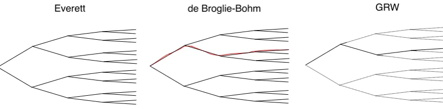
I offer a detailed development of the view that the bulk of technical analysis needed to recover classical behavior from quantum theory is largely independent of the precise features of the collapse mechanism and ontology of the quantum state. The analysis below demonstrates that concerns about wave function collapse and ontology can be addressed as a coda - allbeit a necessary one - to the account of classical behavior suggested by decoherence theory, so that one need not start anew in the recovery of classical behavior with each new interpretation3 of quantum the-ory that is considered. The interpretation-neutral strategy for recovering classical behavior summarized here rests on three central pillars: decoherence, which gener-ates a branching structure from the unitary quantum state evolution, such that the state of the system of interest relative to each branch is well-localized; Ehrenfest’s Theorem for open quantum systems, which ensures that the only branches with non-negligible weight are branches relative to which the system’s trajectory is ap-proximately Newtonian; a decoherence-compatible prescription for collapse, which serves at each moment to select just one of the branches defined by decoherence in accordance with the Born Rule. The underlying physical mechanism (associated
2I will take the term “collapse” here to encompass both real, dynamical collapse processes as
well as processes in which collapse of the quantum state is merely effective or apparent.
3As several authors have noted, different “interpretations” of quantum mechanics, such as
the Everett, de Broglie-Bohm and GRW interpretations, are more properly regarded as separate
with some particular interpretation of quantum mechanics) for this decoherence-compatible collapse is left unspecified.
This analysis counters the notion promulgated by some authors that recovering classical behavior from quantum theory is a highly interpretation-dependent affair. For example, many advocates of the de Broglie-Bohm (dBB) interpretation have defended an approach built entirely around a condition that is more or less unique to dBB theory: namely, the requirement that the “quantum potential” or “quantum force,” which generates deviations of Bohmian trajectories from Newtonian ones, go to zero. 4 Elsewhere, I have argued that the quantum potential is something of a red
herring and that the most transparent route to recovering classicality in dBB theory relies primarily on structures common to many interpretations, which are associated with decoherence theory [41]. The present article extends this analysis of classical behavior beyond the context of dBB theory to consider other realist interpretations as well, including the Everett and GRW interpretations. It also provides a more detailed elaboration of the interpretation-neutral, decoherence-based framework for recovering classical behavior.
2) A Specific Sense of “Reduction”
Second, I show that the interpretation-neutral framework for recovering classical behavior provided by decoherence theory fits a more general model-based picture of inter-theoretic reduction in physics that I have elaborated and defended elsewhere, according to which reduction between theories is based on a more fundamental concept of reduction between two models of a single, fixed system [40]. Here, I un-derstand a “model” to be specified by some choice of mathematical state space (e.g., phase space, Hilbert space) and some additional structures on that space that serve to constrain the behavior of the state (e.g., Hamilton’s equations, Schrodinger’s equation). This approach differs in important respects from the more conventional approach to reduction in physics that seeks to recover one theory simply as a math-ematical limit of another - typically, in the case of quantum-classical relations, by taking the limit~→0 orN → ∞- while recognizing that limits still carry a strong relevance for inter-theory relations in physics. It also differs from approaches to reduction that have been emphasized in the philosophical literature, which aspire to give a completely general account of reduction across the sciences and so fail to cap-ture the strongly mathematical character of reductions within physics specifically. One feature that distinguishes the view of reduction employed here from these other approaches is that, rather than attempting to give criteria for reduction directly betweentheories as these other approaches do, it is grounded in a more fundamen-tal and more local concept of reduction between two models of a single physical system. Moreover, reduction between models of a single system on this approach is an empirical, a posteriori relation between models rather than a formal, a priori relation that can be assessed on purely logical or mathematical grounds. While this account of inter-theoretic reduction incorporates insights about reduction previously highlighted by other accounts, its novelty lies in the particular combination of
fea-4It is possible to define the quantum potential and force in other interpretions, but because these
tures that it possesses: namely, that it is model-based rather than theory-based, “local” rather than “global”, anda posteriori rather than a priori. By highlighting an important sense of reduction and showing how decoherence theory provides a viable framework for effecting this kind of reduction between quantum and classical theories, I seek to provide a counterweight to recent discussions - in particular, by Batterman, Berry and Bokulich - that have urged a move away from thinking about quantum-classical relations as an instance of reduction [5], [6], [10]. In a separate article, I argue that the singular mathematical limits that Batterman and Berry take to block reduction between classical and quantum mechanics do not block reduction between these theories in the particular sense described here [39].
Beyond its defense of these two points, much of the novelty of the present dis-cussion lies in its explicit synthesis of various elements from different parts of the literature on decoherence, the measurement problem and the quantum-classical cor-respondence, and in its attentiveness to nuances that arise when joining these vari-ous elements - from the explicit requirement that an interpretation-neutral collapse prescription be decoherence-compatible, to subtle variations in the decoherence con-ditions required for effective collapse across different interpretations, to the imple-mentation of the open-systems form of Ehrenfest’s Theorem rather than the more commonly discussed but less appropriate closed-system form. The discussion is structured as follows. Section 2 provides an overview of sources in the decoherence literature that attempt to explain the validity of classical equations of motion and highlights points on which the present discussion serves to complement these inves-tigations. Section 3 discusses several important points of terminology and method-ology, including my usage of the term “classical” and a description of the general approach to reduction adopted here. Section 4 describes a framework for recov-ering classical behavior that is based in results from decoherence theory but that remains non-commital as to the precise mechanism for collapse and the ontology of the quantum state. Section 5 shows how the interpretation-neutral account of clas-sical behavior provided by decoherence can be specially tailored to give an account of classicality in the Everett, de Broglie-Bohm and GRW interpretations, thereby resolving - if only in a speculative way - ambiguities associated with collapse in the interpretation-neutral account. Section 6 acknowledges a number of general con-cerns about decoherence-based approaches to recovering classical behavior. Section 7, the Conclusion, briefly considers some broader implications of the analysis given here, including possible extensions of this strategy to the relations between quantum and classical field theory and classical and quantum gravity. The core claims of the article are defended in Sections 3, 4 and 5.
2
Existing Decoherence-Based Accounts of
New-tonian Behavior
dif-fers from, and serves to complement, these other investigations. Generally speaking, none of these sources formulates the decoherence-based account of classical behavior in a way that can be transparently and straightforwardly tailored to accommodate multiple interpretation-dependent collapse mechanisms, and none explicitly frames its analysis of classicality within the more general account of inter-theoretic reduc-tion in physics that I advocate here.
In [2] and [3], Bacciagaluppi describes in verbal, qualitative terms the general approach to recovering classical behavior that I elaborate in more technical detail below. In particular, he regards decoherence theory as an interpretation-neutral body of results that serves to define the range of possible measurement 5 outcomes
associated with different branches of the quantum state, and interpretation-specific collapse mechanisms as serving to select one of these branches in accordance with the Born Rule. 6 Beyond developing this general approach in more technical detail,
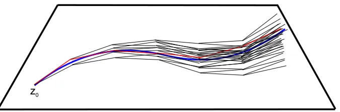
our analysis differs from Bacciagaluppi’s with regard to the particular form of Ehren-fest’s Theorem that it invokes to explain why branch-relative trajectories should be approximately Newtonian. While Bacciagaluppi invokes the familiar closed-systems version of Ehrenfest’s Theorem, our analysis relies on a more germane but less familiar version of this theorem derived by Joos and Zeh for the special class of open systems whose reduced state obeys the Caldeira-Leggett master equation (see [28], Ch.3). Our analysis carries Joos and Zeh’s result further by showing that on timescales where ensemble wave packet spreading of the system in question is suf-ficiently small, the localized, branch-relative state of the system will approximately follow a Newtonian trajectory, deviating from Newtonian form only through small, stochastic, branch-dependent “quantum fluctuations” (see Figure 2).
Zurek has shown how classical equations of motion for probability distributions over phase space can be recovered in open quantum systems undergoing decoherence [66]. In particular, he has argued that as a result of decoherence, the Wigner func-tion representafunc-tion of the state of an open quantum system approximately obeys a classical Fokker-Planck equation, which takes the form of a classical Liouvillle evo-lution combined with a momentum diffusion term. In cases where the corresponding diffusion coefficient is sufficiently small, the evolution of the Wigner function distri-bution approximates the ordinary classical Liouville evolution. Concerning the more fine-grained level of description in terms of individual trajectories rather than distri-butions over phase space, Bhattacharya, Habib and Jacobs and Habib, Shizume and Zurek both note that the Fokker-Planck evolution is equivalent to a Langevin equa-tion driven by Gaussian white noise [7], [24]. The diffusion term that contributes to the distribution dynamics reflects the influence of the additional noise term at the level of the trajectory dynamics. Rather than motivating the introduction of local-ized, stochastic quantum trajectories indirectly through the analysis of phase space probability distributions as these authors do, our discussion extracts these
trajecto-5I understand “measurement” here in a generalized sense that takes measurement to be any
physical interaction that establishes the appropriate sort of correlation between the system of interest and degrees of freedom external to that system. Crucially, a measurement in this sense need not involve an “apparatus” or “observer”.
6As Bacciagaluppi observes in [3], and as I discuss further in Section 5, it is an open question
ries directly from an analysis of the branching structure of the quantum state. This strategy much more readily facilitates the tailoring of decoherence-based results to a variety of different collapse mechanisms and ontologies associated with different interpretations.
Gell-Mann and Hartle approach the recovery of classical equations of motion from the perspective of the decoherent histories framework and the closely related path integral formalism for open quantum systems [20], [26]. They show that the only trajectories of an open quantum system that contribute non-negligibly to its path integral are approximately Newtonian in form. These results are also discussed in the work of Halliwell [25]. As in the preceding analyses, the roles of branching and collapse in the recovery of determinate Newtonian trajectories are not made transparent in these discussions, nor is the signifcance of these results across different interpretations. 7
It is also worth briefly mentioning several other sources that concern the re-covery of approximately Newtonian trajectories within decoherence theory. In [44], Schlosshauer argues that wave packet trajectories should be approximately New-tonian for a narrowly defined set of models and initial conditions, but does not discuss the more general mechanisms and results that give rise to approximately Newtonian trajectories over a wide range of different models and initial conditions, as we do here. In [45], Schlosshauer examines the relationship between decoherence and various interpretations of quantum theory; our discussion in Section 5 below complements Schlosshauer’s by emphasizing that quantitatively different forms of decoherence are needed to induce effective collapse across different interpretations. Landsman’s [31] cites a special role for decoherence in explaining the dynamical origin of coherent states, which he claims are needed to ensure certain correspon-dences in the mathematical limit ~ → 0. However, Landsman’s focus is primarily on mathematical correspondences between the formalisms of quantum and classical mechanics, rather than directly on the quantum mechanical description of classical behavior.
3
Terminology and Methodology
In this section, I clarify several points of terminology and methodology employed in the discussion below. First, I explain my usage of terms such as “classical” and “quasi-classical”. Second, I describe a model-based sense of reduction in physics that I have elaborated in detail elsewhere; in later sections, I argue that decoher-ence theory provides a viable strategy for effecting this type of reduction between quantum and classical mechanics.
7It is worth noting here that Gell-Mann and Hartle regard the formalism of decoherent histories
3.1
The Meaning of “Classical”
The term “classical” carries a range of different meanings across the literature on quantum-classical relations. In the context of recovering classical behavior within quantum theory, I take it to denote the following kinematical and dynamical re-quirements:
Kinematical Requirements
• quasi-classicality: The system in question must possess determinate or approx-imately determinate values for position and momentum simultaneously; within the constraints of the uncertainty principle, it is possible for both quantities to be simultaneously sharply defined relative to macroscopic scales of length and momentum.
• separability: One some level, the state of a system exhibiting classical behavior should be determined completely by the states of its individual subsystems. 8
• “objectivity”: Disjoint subsystems of the environment - including those associ-ated with any observers that may be present - must agree on the quasi-classical values for position, momentum or other variables that they register for the sys-tem of interest. This requires a strong measure of redundancy in the encoding of information about the central system within the environment (see, e.g., [64], [44], Section 2.9 and references therein for further elaboration of this concept of objectivity; see [17] for a critique of this notion).
Dynamical Requirements
• obeying classical equations: Quasi-classical trajectories must approximate the solutions to classical equations of motion over appropriate timescales and within appropriate margins of error. As I discuss below, these timescales and margins of error are constrained by the timescales and margins of error within which the classical model of a system successfully tracks the system’s behavior.
Examples of the sort of system whose classical behavior we seek to model quantum mechanically include the following:
• center of mass of the Moon, planets, etc.
• center of mass of a golf ball, baseball, etc.
• charged particle (e.g., alpha particle, proton, electron) in a bubble chamber or particle accelerator.
8Of course, in quantum theory this is not the case for general states since the density matrix of
It is important to note, as others have, that the set of systems that are well-described by purely classical models includes not only macroscopic bodies but also (as in the last set of examples) bodies of atomic and sub-atomic size. For example, in a particle accelerator or bubble chamber, it is classical equations - specifically, the Lorentz force law - that are used to predict and guide the particles’ motion. It is also worth taking a moment to note that the term “classical” is sometimes used to describe phenomena for which a certainhybrid of quantum and classical concepts is effective - for example, in studies of semi-classical analysis and applications of the WKB approximation in quantum physics (see, for example, [5], Ch.7 and [6]). I do not employ the term in this manner, reserving it instead for behavior that is well-described by models that are exclusively classical and do not contain any reference to quantum mechanical concepts.
3.2
A Local, Empirical, Model-Based Concept of Inter-Theoretic
Reduction in Physics
The term “reduction” is notoriously slippery. In the context of inter-theory relations in physics, the term is often associated with the requirement that one theory be a “limit” or “limiting case” of another. However, as I have argued in detail elsewhere, this requirement is extremely vague since the limit of a theory is not a mathemat-ically well-defined concept (nor, for that matter, is the concept of a theory) and it is far from clear what it means, in general, for one theory to be a limit of an-other [40]. To judge from common occurrences of this manner of speaking, it seems that the limit-based concept of reduction is defined generally by little more than the very weak requirement that somehow, something like a limit be involved in the relationship between some portions of the two theories involved.
difficulty for the Kemeny-Oppenheim account of reduction has been to make this concept of systematization precise, while another has been its heavy reliance on the observational-theoretical distinction, which has been widely discredited since the decline of logical positivism and empiricism. Because they aspire to give accounts of reduction across the sciences and not just in physics, neither the Nagel/Schaffner nor the Kemeny/Oppenheim model of reduction fully captures the specifically math-ematical character of reductions within physics.
Elsewhere, I have argued for an alternative model-based concept of reduction in physics that incorporates important insights from each of these accounts while correcting some of their shortcomings [40]. Rather than defining reduction in physics as a matter of effecting a single wholesale derivation of one theory’s laws from those of another, as the Nagelian and limit-based accounts tend to do, the account of reduction in physics that I propose defines reduction between theories in terms of a more fundamental notion of reduction between two models that represent the same physical system - for example, between the quantum mechanical and quantum field theoretic models of a single electron, or between the classical and quantum models of an everyday object like a baseball. The specification of a model typically consists in the specification of a state space and some dynamical or other constraints on the behavior of these states. For example, in models of quantum mechanics, this entails a commitment to a particular Hilbert space of some specified dimension (that is, assuming a non-algebraic approach to quantum theory) with some particular Hamiltonian defined over it. In models of classical mechanics, it typically entails a commitment to a particular phase space or configuration space of fixed dimension and topology, also with some particular Hamiltonian or Lagrangian. Thus, following van Fraassen and other advocates of the “semantic” view of theories, a theory can be associated with some category of models - for example, in the case of quantum mechanics, the category of models that can be formulated in terms of the unitary evolution of some Hilbert space vector - while a choice of particular model within that category to describe some particular system involves more detailed specifications (e.g., of a specific Hilbert space and Hamiltonian) [54].
Specifically, I take “theory Th reduces to theory Tl” to mean that every
circum-stance under which a real system’s behavior is accurately represented by some model of theory Th is also a circumstance in which that same behavior is represented at
least as accurately, and in at least as fine-grained a way, by some model of theory
Tl. 9 Thus the primary requirement for “reduction” as I use the term here is that
the domain of applicability of the reduced theory be subsumed into that of the re-ducing theory. Because every system in the domain of a theory is represented by some particular model of that theory, this notion of reduction between theories can be understood in terms of the more fundamental notion of reduction between two models of a single system, which I designate reductionM. Reduction between two
theories, reductionT, can be defined in terms of reduction between two models of a
single physical system,reductionM, as follows:
Theory Th reducesT to theory Tl iff for every system S in the domain
of Th - that is, for every physical system S whose behavior is accurately
represented by some model Mh of Th - there exists a modelMl of Tl also
representing S such that Mh reducesM toMl.
ReductionM is a three-place relation between Mh,Mland some real physical system
S 10 , which requires that M
l provide at least as accurate and detailed a
descrip-tion of S’s behavior as Mh in all cases where Mh is successful. Where both models
successfully describe (to within some margin of approximation) the same features of
S, consistency requires a certain dovetailing between the models, which is typically manifested as a certain mathematical relationship between the models. However, it is important to stress that reductionM only requires this dovetailing to occur in
cases where Mh furnishes an accurate representation ofS, and that the models are
permitted to diverge arbitrarily outside of this domain. The particular form of the mathematical relationship between Mh and Ml that underwrites reductionM in a
given case will depend on the general classes of model to which Mh and Ml
be-long. Moreover, this relationship will typically be parametrized by empirical values characterizing the accuracy and scope of Mh in its representation of S. In [40], I
give precise conditions for reductionM in a class of cases where both models are
deterministic dynamical systems, and briefly suggest how these criteria might be generalized. Below, I specify conditions forreductionM in the class of cases relevant
to us here, concerning the reduction of a deterministic dynamical systems model to a stochastic dynamical model.
It is worth highlighting two features of this model-based approach to reduction in physics. First, it is “local” in the sense that it allows reduction between theories to be effected through numerous distinct, context-specific inter-model derivations across different systems or classes of system, rather than requiring the existence of a single “global” derivation that applies uniformly across the entire domain of the high-level theory. Second, this kind of reduction is that it is an a posteriori, or “empirical”, rather than an a priori, or “formal”, relationship between theories/models. While it is often supposed that reduction in physics is solely a feature of the mathematical or logical relationship between two theories or models, the question of whether one representation succeeds at describing the world in all cases where the other does often has an unavoidable empirical component. The distinction between formal and empirical approaches to quantum-classical reduction is discussed further in [39].
10There are at least two ways of clarifying the meaning of the term “physical system”. The first is
In the context of the reduction between classical and quantum models of a single system, the classical model can be formulated as a determinsitic dynamical system while the precise nature of the quantum model is interpretation-dependent - for ex-ample, models of the Everett and dBB interpretations are deterministic while models of GRW theory are stochastic. However, as I explain in detail below, by relying on the branching structure that arises through decoherence, it is possible to define an effective, stochastic model of the branch-relative quantum state evolution that applies across many different interpretations of quantum theory. 11 This effective model assumes a decoherence-compatible type of collapse, but leaves the detailed physical mechanism governing collapse unspecified. What this physical mechanism happens to be varies according to interpretation. Thus, while the reduction of the deterministic classical model to the effective, stochastic quantum model of a sys-tem is an interpretation-neutral affair, the task of underwriting the latter model’s collapse process within a particular interpretation-specific model is not.
The reduction of the classical model to the effective, stochastic quantum model of a systemS falls into the category of inter-model reductions in which a deterministic dynamical systems model is reduced to a stochastic dynamical model sharing the same time parameter. It is possible to state formal requirements forreductionM in
this class of cases that are quite general. Denote the state space ofMhbySh and the
unique time-t evolution of the initial state xh ∈ Sh by Dh(xh, t). Denote the state
space of Ml by Sl and a stochastic time-t evolution of the initial state xl ∈ Sl by
Dl(xl, t). Note thatDl(xl, t) is not a function in the strict mathematical sense since
the time-t evolution of a given initial state does not have a single predetermined value, but emerges probabilistically. Letdh be the set of initial conditions xh inSh
such that Dh(xh, t) tracks the evolution of the system S within margin of error δ
over a time greater than or equal toτ. While there is some flexibility in the choice of values for dh, δ and τ, bounds on these values are empirically constrained by
the quality and scope of fit between Mh and S. Given a triple (δ, τ, dh), reduction
between the models requires that there exist a time-independent function B(xl) 12
from the state spaceSl of the low-level model to the state spaceSh of the high-level
model and some setdl of states inSl such thatB(dl) = dh and for allxl ∈dl,
B(Dl(xl, t))−Dh(B(xl), t)
<2δ, (1)
or less formally,
B(Dl(xl, t))≈Dh(B(xl), t), (2)
for all 0 ≤ t < τ, with probability 1− for very small . 13 The factor of 2 in 2δ
is included because, if the high-level trajectory approximates the system’s evolution to within marginδ and the trajectory induced by the low-level dynamics throughB
11Such effective stochastic quantum evolutions can be modeled using the formalism of quantum
stochastic calculus; see, for example, [18] and [19] for details.
12Note that “time-independent” here means that the functionBis notexplicitly time-dependent;
it may depend indirectly on time through any time dependence ofxl.
Figure 1: In cases where the high-level model of a system is deterministic, the low-level model is stochastic and both models share a time parameter,reductionM requires that the trajectories on Sh induced via B by the low-level dynamics approximate those high-level trajectories that successfully track the behavior of the physical systemS.
also approximates the system’s evolution to within δ, as reductionM requires, then
these trajectories may be separated from each other by as much as 2δ.
Briefly summarized, reductionM in this class of cases requires that with very
high likelihood, the operations of dynamical evolution and application of the “bridge map” or “bridge function”Bapproximatelycommutewithin the relevant empirically determined margins. Equivalently, reductionM requires that all physically salient
high-level trajectories be approximated within appropriate margins by trajectories that areinduced on the high-level state space by the low-level dynamics through the bridge map (see Figure 1). From a physical point of view, this requirement may be interpreted as follows. SincereductionM requires that Ml succeed at describing S’s
behavior in all cases where Mh does, when the evolution of xh successfully tracks
real features of S, there must be some quantity defined within Ml that, with very
high likelihood, tracks these same features at least as accurately. The quantity
B(xl), which is the same type of mathematical object as xh, but whose dynamics
are determined byMl, fills this role if the requirement (2) for reduction holds. Thus,
the requirement (2) helps to ensure thatB(xl) provides an adequate surrogate forxh
in cases whereMh is successful at describing S’s behavior. The possibility of using
3.3
A Few Caveats
The local, model-based, empirical approach to reduction adopted here suggests a precise mathematical criterion for reduction between classical and quantum models of a single system exhibiting classical behavior. These criteria, which follow the general pattern of eq. (1), are formulated in Section 4.7. However, no attempt is made here to provide a rigorous proof that this condition holds across all systems where classical behavior occurs. It is likely that many of the details required to give such a proof will vary across different systems, so that full rigor can only be achieved through specialization to particular systems or classes of system. My goal here is only to outline the centralstrategy offered by decoherence theory for explaining why this condition should hold generally across systems that exhibit classical behavior -that is, to describe a general template into which a more complete derivation could be fit.
4
An Interpretation-Neutral, Decoherence-Based
Strategy for Quantum-Classical Reduction
In this section, I outline an interpretation-neutral, decoherence-based strategy for re-covering classical behavior from quantum theory, which relies heavily on the general approach to reduction outlined in the previous section. In a nutshell, this strategy rests on three central pillars: 1) decoherence to generate a branching structure for the quantum state, such that the state of the system of interest relative to any single branch is always quasi-classical; 2) a decoherence-compatible collapse pre-scription that selects one of these branches in accordance with the Born Rule, and whose underlying physical mechanism is left unspecified; 3) an appropriate form of Ehrenfest’s Theorem to ensure that quasi-classical, branch-relative trajectories are approximately Newtonian over relevant timescales. In Section 5, I show how concerns about the physical mechanism underpinning this decoherence-compatible collapse prescription can be addressed as a coda - albeit a necessary one - to the interpretation-neutral account given in this section, and that interpretation-specific aspects of the quantum mechanical description of classical behavior can therefore be quarantined to a relatively narrow portion of the overall analysis. In other words, we will see how the different collapse mechanisms and ontologies associated with different interpretations can be “slotted in” to this interpretation-neutral account to give a more complete, if more speculative, picture of classical behavior than the one provided by the interpretation-neutral picture alone. Thus, we will see more explicitly than previous investigations how one can go quite far in providing a quantum-mechanical account of classical behavior without taking on the specu-lative metaphysical commitments associated with some particular interpretation of quantum theory. Of course, we must also keep in mind that at most one of these interpretation-specific accounts can be correct as a description of the mechanism that nature itself employs.
basis of coherent states implies decoherence of histories defined with respect to an approximate PVM on phase space. To each such history is associated a branch vector and a corresponding localized (though not necessarily Newtonian) trajectory through classical phase space. Using these branch vectors, it is possible to define an effective, decoherence-compatible prescription for collapse that serves to “black-box” all interpretation-specific details within a single portion of the analysis - where by “decoherence-compatibility” I mean that the outcome of any collapse is some normalized branch vector, and the probability of this outcome occurring conforms to the Born Rule. A form of Ehrenfest’s Theorem derived for open quantum sys-tems implies that stochastic, localized trajectories defined through this effective, decoherence-compatible collapse prescription are overwhelmingly likely to be ap-proximately Newtonian on certain timescales.
4.1
Setup
Decoherence-based models of classical behavior take the system of interest S - say, the center of mass of a baseball - to be embedded in a larger closed system SE, where E consists of all degrees of freedom external to S and is typically referred to as S’s “environment” (e.g., air molecules, photons, dust particles, measuring apparati, human observers). The Hilbert space HSE of SE is the tensor product
of the Hilbert space HS of S and the Hilbert space HE of E. The state of SE,
|Ψi ∈ HSE, is assumed always to evolve according to a Schrodinger equation of the
form,
i∂|Ψi ∂t =
ˆ
HS⊗IˆE + ˆIS⊗HˆE+ ˆHI
|Ψi, (3)
where we have set ~ ≡ 1, ˆHS and ˆHE operate, respectively, on HS and HE, ˆIE is
the identity on HE , ˆIS is the identity on HS, ˆHI operates on states in HS⊗ HE,
and
ˆ
HS =
ˆ
P2
2M +V( ˆX), (4)
with ˆX and ˆP the position and momentum operators on HS. A well-known model
of this form is the model of quantum Brownian motion, in which E consists of many independent oscillators whose position operators are linearly coupled through
ˆ
HI to the position operator of S (see, for example, [28], [44] and [12]). For the
purposes of this discussion, I will assume only that ˆHE and ˆHI are consistent with
a Caldeira-Leggett master equation for the reduced state ˆρ≡T rE[|ΨihΨ|] of S:
idρˆ
dt = [ ˆHS,ρˆ]−iΛ
h
ˆ
X,hX,ˆ ρˆii, (5)
where Λ is a constant that depends on the detailed parameters of ˆHE and ˆHI. The
first term on the right-hand side of this equation generates the unitary evolution of ˆ
be ignored. However, the sort of analysis of classical behavior given here can be straighforwardly generalized to the case where a dissipative term is included in the master equation for ˆρ, the main difference being that the dynamical equations of the corresponding classical model will contain a frictional term in this case. For derivations of the Caldeira-Leggett equation in the context of different models for the unitary evolution of SE, see [44], [28] and references therein.
4.2
Environmental Decoherence and Coherent Pointer States
Assume for the moment that the total system SE begins at t = 0 in a product state |Ψ0i =|ψi ⊗ |φi, where |ψi ∈ HS and |φi ∈ HE. Though the assumption of
an initial product state is unrealistic in cases where the evolution of SE is always unitary and whereS andE interact, analyzing this simple case first is an important step in describing the evolution of more general initial states. In general, such a state will evolve under SE’s unitary dynamics into a state that is entangled. The rate at which the degree of entanglement between the two systems increases depends strongly on the choice of |ψi. Two popular ways to quantify the degree of entanglement between a system and its environment are the von Neumann entropy,
SV N ≡ −T r( ˆρlog( ˆρ)) and the linear entropy, SL = 1 −T r( ˆρ2) (the latter is the
leading approximation to the former when the former is expanded in powers of (1−ρˆ)). Several authors have argued that for the systems of interest to us here, these measures of entanglement increase most slowly when|ψi is a minimum uncertainty coherent state|Q, Pi ∈ HS that is narrowly localized about some values of position
Qand momentumP. Expressed in a position basis for S, these states are Gaussian in form:
ΨQ,P(X)≡ hX|Q, Pi=Ae−α(X−Q) 2
eiP X, (6) where A is an appropriate normalization constant, α determines the position- and momentum-space distribution widths associated with this state and these widths multiply to ~
2. Zurek, Habib and Paz have argued this point for the specific case
where the potential V in S’s self Hamiltonian is that of a harmonic oscillator. 14
Through a method known as thepredictability sieve, they consider the time depen-dence of the linear entropy S(t) for a range of different initial pure states |ψi of S
and find that the |ψi for which S increases most slowly are minimum uncertainty coherent states [65]. More qualitative, heuristic arguments have been used to extend this conclusion to more general choices of potential V; see, for example, [44], Ch.’s 2.8 and 5.2 and [56], Ch. 3. Partly because minimum uncertainty coherent states are narrowly localized both in position and momentum and because they tend to avoid entanglement on longer timescales than other states, they are widely thought to provide a quantum mechanical counterpart to points in classical phase space.
Assuming that the pointer states of S are coherent states, let us consider how this assumption constrains the unitary evolution of the quantum state of SE. My discussion here closely follows [56], Section 3.7. Using the condensed notation Z ≡
14In fact, while we limit our attention here to the case of “pure decoherence” described in (5),
(Q, P), |Zi ≡ |Q, Pi, an arbitrary state of SE at some initial time t = 0 can be expressed in the form,
|χ0i=
Z
dZ0 α(Z0)|Z0i ⊗ |φ(Z0)i (7)
where α(Z0) is an expansion coefficent, |Z0i ∈ HS and |φ(Z0)i ∈ HE. (Note that,
initially, the |φ(Z0)i need not be orthogonal.) After the very brief timescale τD
associated with decoherence, we will have that hφ(Z00)|φ(Z0)i ≈ 0 for Z0 and Z00
sufficiently different. To determine the evolution of the overall state, let us first consider the unitary evolution of a single element of the initial superposition,|Z0i ⊗
|φ(Z0)i, and then use the linearity of the Schrodinger evolution to determine the
evolution of the full state. On the timescale ∆t >> τD over which ˆHS induces
significant changes onHS, a single element of the above superposition evolves as
|Z0i ⊗ |φ(Z0)i ∆t
=⇒ Z
dZ1β(Z0, Z1)|Z1i ⊗ |φ(Z0, Z1)i (8)
wherehφ(Z00, Z10)|φ(Z0, Z1)i ≈0 ifZ0 andZ00, orZ1 andZ10, are sufficiently different.
Likewise, evolving each element of this last superposition forward in time by ∆t, we have
|Z1i ⊗ |φ(Z0, Z1)i ∆t
=⇒ Z
dZ2β(Z0, Z1, Z2)|Z2i ⊗ |φ(Z0, Z1, Z2)i, (9)
where hφ(Z00, Z10, Z20)|φ(Z0, Z1, Z2)i ≈ 0 if Zk and Zk0 are sufficiently different, for
any 0≤k ≤2. Iterating this process N times, we obtain,
|Z0i ⊗ |φ(Z0)i N∆t
=⇒ Z
dZ1...dZN B(Z0, ..., ZN) |ZNi ⊗ |φ(Z0, ..., ZN)i (10)
where
B(Z0, ..., ZN)≡β(Z0, Z1)β(Z0, Z1, Z2) ... β(Z0, Z1, Z2, ..., ZN−1, ZN). (11)
By linearity of the Schrodinger evolution, we then have for the evolution of the arbitrary initial state (7),
|χ(N∆t)i=
Z
dZ0...dZN α(Z0)B(Z0, ..., ZN)|ZNi ⊗ |φ(Z0, ..., ZN)i, (12)
with
hφ(Z00, ..., ZN0 )|φ(Z0, ..., ZN)i ≈0 if ZkandZk0 are sufficiently different, for any 0 ≤k≤N.
(13) Relations (12) and (13) provide a completely general expression for the evolution of the quantum state ofSE up to an arbitrary time N∆t 15 under the assumption
15Here N∆tis implicitly assumed to be less than timescales associated with quantum Poincare
that the coherent states |Zi are the pointer states of S under its interaction with
E. Because the different environmental states |φ(Z0, ..., ZN)i are mutually
orthog-onal for different trajectories (Z0, ..., ZN), each such environmental state serves in a
sense to record the sequence or history of localized states of S associated with this trajectory, (|Z0i,|Z1i, ...,|ZNi). Note that this trajectory, while localized, need not
be approximately Newtonian.
4.3
Environmental Decoherence and Decoherent Histories
The formalism of decoherent histories is useful for describing the branching structure that the quantum state acquires as a result of environmental decoherence. I briefly and informally review the basic elements of this framework, including the mathemat-ical concepts of projection-valued measure (PVM), positive operator-valued measure (POVM), history operators, and decoherence of histories.
4.3.1 PVM’s and POVM’s
A projection-valued measure (PVM) on a Hilbert space H is a set of self-adjoint operators{Pˆα} on H such that
X
α
ˆ
Pα = ˆI, (14)
ˆ
PαPˆβ =δαβPˆα, (15)
where there is no summation over repeated indices. The concept of a positive operator-valued measure (POVM) on H generalizes the notion of a PVM by re-laxing the requirement of orthogonality in (15). Thus, a positive-operator-valued measure (POVM) on a Hilbert spaceH is a set{Πˆα}of positive operators such that
X
α
ˆ
Πα = ˆI. (16)
An operator ˆO is positive if it is self-adjoint and hΨ|Oˆ|Ψi ≥ 0 for every |Ψi ∈ H. Note that every PVM is also a POVM.16
4.3.2 An Approximate PVM Constructed from Coherent States
Following Ch. 3 of Wallace’s [56], consider a partition {µα} of the classical phase
space ΓS of the system S introduced in Section 4.1. To such a partition we can
associate the POVM {Πˆα} onHS, where the operators ˆΠα are defined by
ˆ Πα ≡
Z
µα
dZ |ZihZ|. (17)
16See [35] or [14] for a more comprehensive introduction to PVM- and POVM-based treatments
Assuming that the cells µα = uαx ×uαp of the partition have configuration space
volume dX ≡ vol(uαx) and momentum space volume dP ≡ vol(uαp) larger than
those associated with a coherent pointer state, the operators in this POVM will also constitute an approximate PVM, so that
ˆ
ΠαΠˆβ ≈δαβΠˆα. (18)
We can then extend the set {Πˆα} to an approximate PVM on HSE by defining
the set of operators {Pˆα}, where ˆPα ≡ Πˆα ⊗IˆE, with ˆIE the identity on HE. It
is worth emphasizing that the classical phase space ΓS employed in defining this
approximate PVM is not assumed to have any fundamental ontological status, but rather is employed simply as a mathematical tool in defining a structure that is fundamentally quantum mechanical. The fact that this particular PVM is useful for analyzing the branching structure of the pure state evolution ofSE follows from the fact that the coherent states are pointer states of S under its interaction with
E, which in turn follows from the form of SE’s quantum Hamiltonian.
4.3.3 Decoherent Histories
The approximate coherent state PVM just defined is useful for describing the branch-ing structure that emerges from the unitary quantum state evolution through deco-herence. Let us consider the evolution ofSE’s state |Ψiup to some arbitrary time
t >> τD, dividing t into N equal intervals ∆t >> τD, so that t=N∆t:
|Ψ(N∆t)i=e−iHN∆tˆ |Ψ0i (19)
= X
αN
ˆ
PαN
!
e−iH∆tˆ
X
αN−1
ˆ
PαN−1
...e
−iH∆tˆ X
α1
ˆ
Pα1
!
e−iH∆tˆ X
α0
ˆ
Pα0
!
|Ψ0i
(20)
= X
α0,...,αN
ˆ
PαNe
−i
~H∆tˆ Pˆα
N−1...e
−iH∆tˆ Pˆ α1e−
i
~H∆tˆ Pˆα0|Ψ0i (21)
= X
α0,...,αN
ˆ
Cα0...αN|Ψ0i (22)
where ˆCα0...αN ≡PˆαNe
−i
~Hˆ∆tPˆα
N−1...e
−iHˆ∆tPˆ α1e−
i
~Hˆ∆tPˆα0 and in going from the first
to the second line we have used the fact that P
αi
ˆ
Pαi = ˆISE. Each component
ˆ
Cα0...αN|Ψ0i corresponds to a particular history or sequence (µα0, ..., µαN) of regions
through phase space. I will further assume that the same partition {µα} is used
to define the set of approximate PVM operators { Pˆαi } at all times i∆t, where
0≤i≤N. The two histories (α0, ..., αN) and (α00, ..., α
0
N) are said to be decoherent
if the corresponding Hilbert space vectors are orthogonal - that is, if
hΨ0|Cˆ
†
α0 0α01...α0N
ˆ
Cα0α1...αN|Ψ0i ≈0 (23)
forαk6=α0kfor any 0≤k ≤N (this condition is sometimes designated “medium
is called decoherent if any two distinct histories in the set are decoherent. A history is said to be realized if its corresponding Hilbert space vector has non-negligible weight - that is, if |Cˆα0...αN|Ψ0i| ≥ for some small threshold value . Any history
that is not realized is automatically decoherent with respect to every other history, since the inner product of the associated component of the quantum state vector with any other such component will be zero. As Paz and Zurek have argued, and as one can see for oneself by expanding the vectors ˆCα0...αN|Ψ0iin terms of coherent
states using the definition (17) of the operators ˆΠαi, environmental decoherence
rel-ative to a coherent state pointer basis forS, as expressed in (13), entails decoherence of different phase space histories, as expressed in (23) [37].
4.4
Decoherence, Branching and the Unitary Quantum State
Evolution
If the condition (23) is satisfied at all timesN∆tfor different N, the unitary evolu-tion considered at successive time steps takes the form,
|Ψ(0)i=|Ψ0i
|Ψ(τD)i=
X
α0
ˆ
Cα0|Ψ0i
hΨ0|Cˆ
†
α0 0
ˆ
Cα0|Ψ0i ≈0 if α0 6=α00
|Ψ(∆t)i= X
α0,α1
ˆ
Cα0α1|Ψ0i
hΨ0|Cˆ
†
α0 0α01
ˆ
Cα0α1|Ψ0i ≈0if αi =6 α0i f or 0≤i≤1
|Ψ(2∆t)i= X
α0,α1,α2
ˆ
Cα0α1α2|Ψ0i
hΨ0|Cˆ
†
α00α01α02Cˆα0α1α2|Ψ0i ≈0if αi 6=α
0
i f or 0≤i≤2
.. .
|Ψ(N∆t)i= X
α0,α1,α2,...,αN
ˆ
Cα0α1α2...αN|Ψ0i
hΨ0|Cˆ
†
α0
0α01α02...α0N
ˆ
Cα0α1α2...αN|Ψ0i ≈0 if αi 6=α
0
i f or 0≤i≤N,
where ˆCα0 ≡ e−i ˆ HτDPˆ
α0. 17 The unitary evolution in this case exhibits a tree-like
structure in that the probability that one of the mutually decohered components
17Note that it is necessary to evolve the total state forward by the decoherence time τ
ˆ
Cα0...αi|Ψ0i of the total quantum state at time i∆t transitions into the component
ˆ
Cβ0...βiβi+1|Ψ0i at time (i+ 1)∆t is effectively zero unless (β0, ..., βi) = (α0, ..., αi) 18
. That is, the unitary evolution of the vector ˆCα0...αi|Ψ0i will give rise to multiple
distinct, mutually decohered vectors ˆCα0...αiαi+1|Ψ0i (one for each αi+1) at future
times, but the initial segments of the histories associated with those future vec-tors must coincide with the history (α0, ..., αi) of their parent vector. 19 For this
reason, the ˆCα0...αi|Ψ0i are sometimes called branch vectors and the corresponding
normalized states branch states. Let us further stipulate that these branch vectors should be maximally fine-grained with respect toSin the sense that the phase space regions µα used to define the approximate coherent state PVM {Pˆα} should be as
small as possible consistent with (18) and with different histories (α0, ..., αi) being
mutually decohered at each timei∆t. In this case, the dimensionsdX and dP of the
partition cells µα should not be much greater, respectively, than the position- and
momentum-space widths of a coherent pointer state, and the phase space volume
dXdP should not be much larger than 1 - or, equivalently,~n (where, recall, we have
set ~ ≡ 1). Note that ~n = 1 represents the volume in S’s phase space associated with a single coherent state, assuming thatS’s phase space has dimension 2n.
4.5
Effective, Stochastic, Quasiclassical State Evolution
Within the decoherence literature, the world of experience is widely thought to be described at any given time by just one of the quasi-classical branches that arise in the unitary evolution ofSE’s total quantum state. To each branch at each time, we can formally assign an effective, normalized “branch state”,
1
Wα0...αN
ˆ
Cα0...αN|Ψ0i, (24)
whereWα0...αN ≡
q hΨ0|Cˆ
†
α0...αNCˆα0...αN|Ψ0i. Given the unitary branching evolution
just described, we may formally define the following effective, stochastic evolution for the branch state of SE:
1
Wα0
ˆ
Cα0|Ψ0i
prob.|Wα0α1|2 |Wα0|2
−−−−−−−−→ 1
Wα0α1
ˆ
Cα0α1|Ψ0i
prob.|Wα0α1α2|2 |Wα0α1|2
−−−−−−−−−→ 1
Wα0α1α2
ˆ
Cα0α1α2|Ψ0i
prob.|Wα0α1α2α3|2 |Wα0α1α2|2
−−−−−−−−−−−→
...
prob.|Wα0α1α2...αN−1αN| 2 |Wα0α1α2...αN−1|2
−−−−−−−−−−−−−−−→ 1
Wα0α1α2...αN
ˆ
Cα0α1...αN|Ψ0i
prob.|Wα0α1α2...αN−1αN αN+1| 2 |Wα0α1α2...αN−1αN|2
−−−−−−−−−−−−−−−−−−→ ....
(25)
18To calculate the transition amplitude, apply the evolution operator e−iHˆ∆t to the
vector Cˆα0...αi|Ψ0i, followed by the identity operator in the form
P αi+1
ˆ
Pαi+1, yielding
P αi+1
ˆ
Cα0...αiαi+1|Ψ0i. Take the inner product of the resultant vector with ˆCβ0...βiβi+1|Ψ0i for
arbitrary (β0, ..., βi, βi+1). Decoherence of histories at time (i+ 1)∆tensures that this inner
prod-uct will be zero unless (β0, ..., βi) = (α0, ..., αi).
Each step in this evolution,
1
Wα0...αi
ˆ
Cα0...αi|Ψ0i
prob. |Wα0...αiαi+1| 2 |Wα1...αi|2
−−−−−−−−−−−−→ 1
Wα1...αiαi+1
ˆ
Cα1...αiαi+1|Ψ0i. (26)
may be regarded as a combination of a unitary, deterministic branching process,
1
Wα0...αi
ˆ
Cα0...αi|Ψ0i
e−iHˆ∆t
−−−−→ 1
Wα0...αi
X
αi+1
ˆ
Cα0...αiαi+1|Ψ0i, (27)
where hΨ0|Cˆα†0 0...α0iα
0
i+1
ˆ
Cα1...αiαi+1|Ψ0i ≈ 0 if αj 6= α
0
j for any 0 ≤ k ≤ i+ 1, and a
non-unitary, stochastic collapse process,
1
Wα0...αi
X
αi+1
ˆ
Cα0...αiαi+1|Ψ0i
prob.|Wα0...αiαi+1| 2 |Wα0...αi|2
−−−−−−−−−−−→ 1
Wα0...αiαi+1
ˆ
Cα0...αiαi+1|Ψ0i. (28)
It is straightforward to see that the collapse probability |Wα0...αiαi+1| 2
|Wα0...αi|2 coincides with
the Born Rule. Though ad hoc, this collapse prescription is more precise than the prescription appearing in most quantum mechanics texts in that it is explicitly required to be decoherence-compatible - that is, the only allowed outcomes of a collapse process under this prescription are branch states defined by decoherence, whereas the more conventional textbook prescription makes no mention of decoher-ence 20. It is also important to note that the square modulus |W
α1,α2,...,αi|
2 of the
branch state ˆCα1α2...αi|Ψ0i is equal to the probability of the sequence
1 Wα0
ˆ
Cα0|Ψ0i, 1
Wα0α1
ˆ
Cα0α1|Ψ0i, ... , W 1
α0α1...αi−1
ˆ
Cα0α1...αi−1|Ψ0i,
1 Wα0α1...αi−1αi
ˆ
Cα0α1...αi−1αi|Ψ0ion our
effective stochastic evolution 21. Thus, the unitary branching structure described
20See, for example, [34], [42] and [22]. Schwabl’s [46] is something of an exception in that
it includes a short discussion of decoherence-based models of quantum measurement (thanks to Michel Janssen for pointing me to Schwabl’s text).
21To see this, recall that the square modulus of ˆC
α1α2...αN|Ψ0i is equal, by definition, to the
quantity |Wα1α2...αN|
2. Let us now independently calculate the probability of the sequence of
states in (25) according to our effective branch-relative state evolution. This probability is simply
equal to the product of the probabilities |Wα1,α2,...,αi,αi+1|2
|Wα1,α2,...,αi|2 for all transitions (α1, α2, ..., αi) →
(α1, α2, ..., αi, αi+1):
|Wα1α2| 2
|Wα1| 2 ×
|Wα1α2α3| 2
|Wα1α2|
2 ×...×
|Wα1α2...αN−2αN−1| 2
|Wα1α2...αN−2|
2 ×
|Wα1α2...αN−1αN| 2
|Wα1α2...αN−1|
2 (29)
(30)
=|Wα1α2...αN|
2. (31)
By a series of simple cancellations, we can see that the probability on the left-hand side is equal to the square modulus of the branch weight|Wα1α2...αN|
in Section 4.4 formally encodes every possible 22 evolution allowed by our effective,
stochastic branch-state evolution as well as the probability of every such evolution. The stochastic evolution (25) implies a corresponding evolution of the branch-relative reduced density matrix ofS. Definingρˆα0...αn≡|Wα 1
0...αn|2
T rE(Cˆα0...αn|Ψ0ihΨ0|Cˆ†α0...αn),
this evolution is
ˆ
ρα0 −→ρˆα0α1 −→ρˆα0α1α2 −→ ... −→ρˆα0α1α2...αN −→ .... (32)
The states ˆρα0...αiare quasi-classical in that the distributionρα1...αi(X)≡ hX|ρˆα1...αi|Xi
overS’s position is narrowly peaked on the scaledX while the distribution ˜ρα1...αi(P)≡
hP|ρˆα1...αi|PioverS’s momentum is narrowly peaked on the scaledP (recall thatdX
anddP are the position- and momentum-space dimensions of the partition cellµαi).
To each such state, there corresponds a unique past sequence ˆρα0,ρˆα0α1, ...,ρˆα0α1...αi−1
of quasi-classical states from which it must have evolved according to the effective stochastic dynamics, but many possible future sequences of branch-relative quasi-classical states to which it may give rise. Note that the discreteness of the timesteps ∆tis an artefact of the manner in which we have chosen to describe an evolution that occurs continuously in time. Defining the stochastic trajectory ˆρα(N∆t)≡ρˆα0...αN,
where ˆρα0...αN is the outcome of theN
th“collapse”, we can see that when we make the
time intervals ∆t successively smaller - and N successively larger for fixed t - our discrete, stochastic, reduced-state trajectory provides successively better approxi-mations to a continuous, stochastic quasiclassical trajectory of reduced 23 states,
ˆ
ρα(t).
4.6
Quantum Trajectories in Classical Phase Space
The sequence (32) induces a stochastic trajectory on the classical phase space of
S when we take branch-relative expectation values of S’s position and momentum operators:
22At the coarse level of description where interpretation-specific details of collapse are omitted,
there is a correspondingly coarse sense of “possibility” on which future descendents of one’s current branch all represent distinct possible future evolutions, and on which branches other than the one that happens to have been realized could have possibly been realized instead. Of course, the precise sense in which other branches could have been realized, and in which future descendents of one’s current branch represent possible future evolutions, varies across interpretations. In dBB theory, for example, the future branch is completely predetermined by an exact specification of the Bohmian configuration and the quantum state; thus, the sense in which other branches are possible requires us to imagine alternative values for the present Bohmian configurations. In GRW theory, by contrast, there is a sense in which the future branch-relative evolution is completely open and not determined by any details of the present state of the world. It is the coarse, effective sense of possibility, rather than the more precise sense associated with any particular interpretation, that I invoke in the present context.
23Note that “reduced” here is intended in the sense of “reduced density matrix” - that is, to
Xα0...αN ≡
1
|Wα0...αN|
2hΨ0|Cˆ
†
α0...αN
ˆ
X⊗IˆE
ˆ
Cα0...αN|Ψ0i=T rS
ˆ
ρα0...αNXˆ
Pα0...αN ≡
1
|Wα0...αN|
2hΨ0|Cˆ
†
α0...αN
ˆ
P ⊗IˆE
ˆ
Cα0...αN|Ψ0i=T rS
ˆ
ρα0...αNPˆ
,
or, more concisely,
Zα0...αN ≡
1
|Wα0...αN|
2hΨ0|Cˆ
†
α0...αN
ˆ
Z⊗IˆE
ˆ
Cα0...αN|Ψ0i=T rS
ˆ
ρα0...αNZˆ
(33) where Zα0...αN ≡ (Xα0...αN, Pα0...αN) ∈ µαN and ˆZ ≡ ( ˆX,Pˆ). The trajectory in
classical phase space induced by the stochastic evolution (32) is
Zα0 −→ Zα0α1 −→ Zα0α1α2 −→ ... −→ Zα0α1α2...αN −→ ... .
As in Section 5.1, we may take the time intervals ∆t successively smaller in order to approximate a continuous trajectory Zq(t) ≡ T r
S[ ˆρα(t) ˆZ], where Zq(N∆t) =
Zα0...αN =T rS[ ˆρα0...αNZˆ].
4.7
Why
Newtonian
Trajectories? Dynamical Requirements
for Inter-Model Reduction
Within the decoherence literature, it is often thought that the determinate, quasi-classical states of affairs that characterize the world of our experience are represented by individual branches of the total quantum state. Thus, it is natural to suppose that the physical degrees of freedom that are represented in classical models by a point in phase space should be represented in the corresponding quantum model by branch-relative expectation values of position and momentum, around which the branch-relative distributions in these quantities are tightly peaked. Assuming that this is the case, there remains the further question of why, in cases where the system
S is the center of mass of a body such as the moon, a baseball, or an alpha particle, the evolution of these branch-relative expectation values according to the effective, stochastic quantum evolution described above should, with very high likelihood, approximate some solution to Newton’s equations of motion.
We can pose the question more formally and precisely within the context of the local, empirical, model-based approach to reduction described in Section 3.2. The state space of the high-level model Mh in this case is the classical phase
space ΓS of the system S. The high-level dynamics are prescribed by the
the state space of the low-level model to be the space Q(HS) of density matrices
on the Hilbert space of the system S and the low-level dynamics to be given by (32), which in turn is derived from the prescription (25). 24 Let d
c denote the
domain of states in ΓS such that Hamiltonian trajectories with initial conditions in
dctrack S’s behavior within margin of errorδZ over a timescale greater than τc. As
noted in Section 3.2, there will be some flexibility in the valuesδZ,τcand dc, which
parametrize the fit between the classical model and the behavior of the system S. Fixing values for (δZ, τc, dc), letZc(t, Z0) represent the deterministic classical
trajec-tory with initial condition Z0 ∈dc and Zq(t,ρˆ0) represent a phase space trajectory
induced by the stochastic quantum evolution of the initial state ˆρ0. Furthermore,
assume that Z0 =T rS
h
ˆ
ρ0Zˆ
i
, so that both the classical and induced quantum tra-jectories have the same starting point in ΓS at t = 0. Following the discussion of
Section 3.2,reductionM of our deterministic classical model to our effective
stochas-tic quantum model requires that for each Z0 ∈ dc, there exist a ˆρ0 ∈ Q(HS) such
that T rS[ ˆρ0Zˆ] =Z0 and, with probability 1− for very small ,
Zq(t,ρˆ0)−Zc(t, Z0)
<2δZ (34)
or, more explicitly,
T rS
h
ˆ
ρα(t) ˆZ
i
−Zc(t, Z0)
<2δZ (35)
for 0 ≤ t < τc. Denote by dqthe set of all such ˆρ0. In this example, the bridge
function B appearing in Eq. (1) is given by B( ˆρ) = T rS
h
ˆ
ρZˆi. We will see below that the domaindq⊂ Q(HS) consists of states ˆρ0 that are narrowly peaked in both
their position and momentum ensemble widths. We now set ourselves to outlining an argument as to why condition (34) should hold under circumstances where classical behavior is known to occur, so that the quantum model gives at least as accurate (if not necessarily as convenient) a representation of the system’s behavior as the classical model in these cases.
4.8
Ehrenfest’s Theorem for Open Quantum Systems
Our approach to showing that condition (34) holds in relevant cases lies in a certain extension of Ehrenfest’s Theorem to open quantum systems that was first derived (as far as I know) by Joos and Zeh (see [28], Ch.3). In order to highlight the novel aspects of this approach, let us begin by reviewing the well-known attempt to recover classical behavior based on the much more commonly cited closed-system form of Ehrenfest’s Theorem.
In its familiar form, Ehrenfest’s Theorem applies only to cases where the system of interestS is closed and in a pure state, and where its evolution is always governed
24While the distinction between a physical system and its representations by different models
by a Schrodinger equation with Hamiltonian ˆH = Pˆ2
2M +V( ˆX). The theorem, which
follows immediately from taking the expectation value of the Heisenberg equation of motion for momentum, states that given these assumptions, the following relation holds for all times t and all states|ψi:
dhPˆi
dt =−h
ˆ
∂V(X)
∂X i. (36)
Combined with the relation dhdtXˆi =hPˆ
Mi(the expectation of the Heisenberg equation
for position), this impliesd2dthX2ˆi =−h
ˆ
∂V(X)
∂X i. Note that despite its formal resemblance
to Newton’s second law of motion, this last relation doesnot entail that expectation values of position and momentum evolve approximately classically. For that to
be the case, it is necessary that d2dthX2ˆi = − ∂V(hXˆi)
∂hXˆi =
∂V(X) ∂X
hˆ
Xi
. If we impose the
restriction that |ψi be a wave packet whose spatial width is narrow by comparison with the characteristic length scales of the potential V, it follows that
dhPˆi
dt ≈ −
∂V(X)
∂X
hXˆi
, (37)
which, together with the relation dhdtXˆi = hMPˆi, entails that this condition is satisfied approximately. The relation (37), in turn, can typically only be expected to hold for as long as|ψ(X)|2 remains suitably narrowly peaked by comparison with the
di-mensions ofV. Except in the special case whereV is a harmonic oscillator potential - in which case the relation (37) is satisfied with exact equality for all states at all times, and coherent states maintain their width - quantum mechanical wave packets can generally be expected to spread out over time.
For systems that are open, as is the case for real systems that exhibit classical behavior, the assumption that S is always in a pure state and that the dynamics of S’s state are always unitary does not apply. Taking quantum mechanics as a universal theory, interaction of such systems with microscopic degrees of freedom in their environments is unavoidable, so that our quantum model of S must allow for the possibility of entanglement with its environmentE. Taking the state of S then to be given by the reduced density matrix ˆρand to evolve according to the canonical master equation (5), and using the relationshPˆi=T r[ ˆρPˆ] and hXˆi=T r[ ˆρXˆ], Joos and Zeh have shown that
d T rS[ ˆρPˆ]
dt =−T rS
"
ˆ
ρ
ˆ
∂V(X)
∂X
#
, (38)
or more concisely,
dhPˆi
dt =−h
ˆ
∂V(X)
∂X i, (39)