Identification of protein functions using a machine-learning approach based on sequence-derived properties

(1)

Open Access

Research

Identification of protein functions using a machine-learning

approach based on sequence-derived properties

Bum Ju Lee

1

_{, Moon Sun Shin}

2

_{, Young Joon Oh}

1

_{, Hae Seok Oh}

3

_and

Keun Ho Ryu*

4

Address: 1_{Industrial Research Center, Jungwon University, 5 Dongbu-ri, Goesan-eup, Goesan-gun, Chungbuk 367-805, Republic of Korea,}2_Dept. of Computer Science, Konkuk University, 322 Danwol-Dong, Chungju-Si, Chungbuk 380-701, Republic of Korea, 3_{Dept. of Computer Science,} Kyungwon University, 161 Bokjung-Dong, Soojung-Gu, Seongnam-Si, Gyeonggi-Do 461-701, Republic of Korea and 4_{School of Electrical and} Computer Engineering, Chungbuk National University, 12 Gaeshindong, Cheongju, Chungbuk 361-763, Republic of Korea

Email: Bum Ju Lee - [email protected]; Moon Sun Shin - [email protected]; Young Joon Oh - [email protected]; Hae Seok Oh - [email protected]; Keun Ho Ryu* - [email protected]

* Corresponding author

Abstract

Background: Predicting the function of an unknown protein is an essential goal in bioinformatics. Sequence similarity-based approaches are widely used for function prediction; however, they are often inadequate in the absence of similar sequences or when the sequence similarity among known protein sequences is statistically weak. This study aimed to develop an accurate prediction method for identifying protein function, irrespective of sequence and structural similarities.

Results: A highly accurate prediction method capable of identifying protein function, based solely on protein sequence properties, is described. This method analyses and identifies specific features of the protein sequence that are highly correlated with certain protein functions and determines the combination of protein sequence features that best characterises protein function. Thirty-three features that represent subtle differences in local regions and full regions of the protein sequences were introduced. On the basis of 484 features extracted solely from the protein sequence, models were built to predict the functions of 11 different proteins from a broad range of cellular components, molecular functions, and biological processes. The accuracy of protein function prediction using random forests with feature selection ranged from 94.23% to 100%. The local sequence information was found to have a broad range of applicability in predicting protein function.

Conclusion: We present an accurate prediction method using a machine-learning approach based solely on protein sequence properties. The primary contribution of this paper is to propose new PNPRD features representing global and/or local differences in sequences, based on positively and/ or negatively charged residues, to assist in predicting protein function. In addition, we identified a compact and useful feature subset for predicting the function of various proteins. Our results indicate that sequence-based classifiers can provide good results among a broad range of proteins, that the proposed features are useful in predicting several functions, and that the combination of our and traditional features may support the creation of a discriminative feature set for specific protein functions.

Published: 9 August 2009

Proteome Science 2009, 7:27 doi:10.1186/1477-5956-7-27

Received: 13 March 2009 Accepted: 9 August 2009

This article is available from: http://www.proteomesci.com/content/7/1/27

(2)

Background

The need to analyse the massive accumulation of biologi-cal data generated by high-throughput human genome projects has stimulated the development of new and rapid computational methods. Computational approaches for predicting and classifying protein functions are essential in determining the functions of unknown proteins in a faster and more cost-effective manner, because experi-mentally determining protein function is both costly and time-consuming. Approaches based on sequence and structure comparisons play an important role in predict-ing and classifypredict-ing the function of unknown proteins. Generally, if an unknown gene or protein sequence is identified, researchers may carry out a sequence similarity search using BLAST [1], PSI-BLAST [2], or FASTA [3] to find similar proteins or annotation information in public databases. However, proteins that have diverged from a common ancestral gene may have the same function but different sequences [4,5]. As a result, sequence similarity-based approaches are often inadequate in the absence of similar sequences or when the sequence similarity among known protein sequences is statistically weak (called the "twilight zone" or "midnight zone") [6-12]. Thus, researchers should be cautious when using this approach, because its efficiency is limited by the availability of anno-tated sequences in public databases and a high-similarity BLAST search result does not always imply homology [13,14]. Structure similarity-based approaches – such as Deli[15] or MATRAS [16], both of which use structure comparisons – have routinely been used to identify pro-teins with similar structures, because protein structural information is better conserved than sequence informa-tion [17,18]. Nevertheless, proteins with the same func-tion can have different structures, and a structural comparison through structure determination is more dif-ficult than a sequence comparison [9,19,20].

Recently, several researchers have developed methods for classifying and predicting protein function independent of sequence or structural alignment [5-9,20-50]. Rather than making predictions based on direct sequence or structural comparisons, these approaches use various fea-tures to predict protein function, such as protein length, molecular weight, number of atoms, grand average of hydropathicity (GRAVY), amino acid composition, perio-dicity, physicochemical properties, predicted secondary structures, subcellular location, sequence motifs or highly conserved regions, and annotations in protein databases. These features include statistics extracted from the protein sequence, structure, and annotation. In addition, to obtain good predictive power, various machine-learning algorithms such as support vector machines (SVMs), neu-ral networks, naïve Bayes classifiers, and ensemble

classi-fiers have been used to build classification and prediction models. Of these, the most widely used machine-learning algorithm for classification and prediction of protein function is SVM [5-7,22,26,27,29,31,36,39-43,45].

A method for classifying the functions of homodimeric, drug absorption, drug delivery, drug excretion, and RNA-binding proteins, among others, has been proposed by Cai et al. [29]. Classification of protein function was per-formed using an SVM statistical learning algorithm, based on features such as amino acid composition, hydropho-bicity, solvent accessibility, secondary structure, surface tension, charge, polarisability, polarity, and normalised van der Waals volume. Cai et al. [29] found that the testing accuracy of protein classification was in the range 84–96% and suggested that amino acid composition, hydropho-bicity, polarity, and charge play more critical roles than other features. Recently, Tung et al. [40] proposed a pre-diction method for ubiquitylation sites using three data-sets (amino acid identity, physicochemical properties, and evolutionary information) and three machine-learn-ing algorithms (k-nearest neighbour, SVM, and naïve Bayes). The greatest accuracy (72.19%) was obtained using SVM with 531 physicochemical properties as fea-tures. Moreover, accuracy improved from 72.19% to 84.44% when 31 physicochemical properties were selected and used based on feature selection by an inform-ative physicochemical property mining algorithm (IPMA). In addition, Li et al. [45] demonstrated the ability of the SVM prediction method to identify potential drug targets. On the basis of amino acid composition, hydro-phobicity, polarity, polarisability, charge, solvent accessi-bility, and normalised van der Waals volume, they obtained an accuracy of 84% in predicting known drug targets versus putative nondrug targets. In that study, the performance of the SVM model did not change signifi-cantly with a greater number of negative targets, as deter-mined from experiments using various ratios of negative to positive samples.

(3)

hydro-phobicity, and they concluded that the best performing feature was phyletic retention or the presence of an ortho-logue in other organisms.

Neural networks are also frequently used for function pre-diction [23-25,36]. For example, six enzyme classes and enzymes/nonenzymes were predicted by Jensen et al. [24], based solely on a few meaningful features such as O-β -GlcNAcsites, N-linked glycosylation, secondary structure, and physicochemical properties. Function prediction was carried out using a neural network, and certain meaning-ful features – such as differences in secondary structures between enzymes and nonenzymes – were analysed. The discriminative ability of each feature was represented by its correlation coefficient.

Ensemble classifiers have recently become popular for protein function classification [25,35,46,47,51-55]. Zhao

et al. [35] suggested that no single-classifier method can always outperform other methods and that ensemble clas-sifier methods outperform other clasclas-sifier methods because they use various types of complementary infor-mation. In comparing the performance of classifiers for predicting glycosylation sites, Caragea et al. [52] demon-strated that ensembles of SVM classifiers outperformed single SMV classifiers. In addition, Guan et al. [51] illus-trated the benefits of using an SVM-based ensemble framework by analysing the performance of ensembles of three classifiers as a single SVM, a hierarchically corrected combination of SVMs, and naïve Bayes classifiers. Ge et al. [53] provided evidence that ensemble classifiers outper-form single decision tree classifiers by comparing C4.5 with several ensemble classifiers (i.e. random forest, stacked generalisation, bagging, AdaBoost, LogitBoost, and MultiBoost) for classification of premalignant pan-creatic cancer mass-spectrometry data. A prediction method using a domain-based random forest of decision trees to infer protein-protein interactions (PPIs) was pro-posed by Chen et al.[46]; in experiments using a Saccharo-myces cerevisiae dataset, they showed that the random-forest method achieved higher sensitivity (79.78%) and specificity (64.38%) than maximum likelihood estima-tion (MLE).

These previous studies exploit direct relationships between basic protein properties and their functions to predict protein function without consideration of sequence or structural similarities. Among these studies, a wide variety of features or only a few meaningful features were selected to increase the performance of function pre-diction based on experience or a few heuristics. However, in most of the previous studies, features that represent subtle distinctions in small portions of protein sequences have not been sufficiently represented. Although proteins share similar structural organisations, biological proper-ties, and sequences, small changes in amino acids of a

protein sequence can result in different functions [19,20,56]. Although local information such as the pres-ence of motifs or highly conserved regions is useful for function prediction, motif detection problems present another arduous task. Therefore, in this study, a method was developed to detect small changes in amino acids within a sequence.

The method described here is characterised by three pri-mary features designed to address specific problems inherent in protein function prediction. First, this approach was designed to accurately predict various pro-tein functions over a broad range of cellular components, molecular functions, and biological processes without using sequence or structural similarity information. Sec-ond, this study was designed to determine whether the use of feature selection improves prediction performance for various protein functions. In other words, does the use of more features related to the protein sequence increase the accuracy of prediction? Third, this study was designed to determine whether local information for the protein sequence is meaningful in predicting protein function, and if so, to determine which features are correlated with protein function.

In summary, a highly accurate prediction method capable of identifying protein function is proposed. One of the advantages of this method is that it requires only the pro-tein sequence for feature extraction; information vis-à-vis

predicted features or structural properties is not required. In addition, four features that represent subtle differences in local regions of the protein sequence – differences due to positively and negatively charged residues – are intro-duced. A total of 484 features, including 451 traditional features and 33 features introduced in this study, were used to predict 11 protein functions. We applied two machine-learning algorithms (i.e. SVM and random for-ests) with and without feature selection to the data set to predict protein function. The prediction performance for each protein function was evaluated, and the features most relevant to prediction of specific protein functions were determined.

Methods

Data preparation

(4)

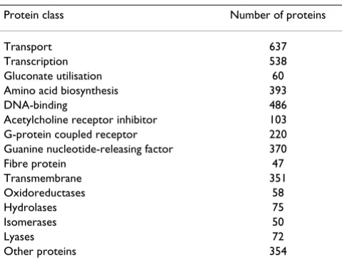
that do not belong to that class and from enzyme families such as oxidoreductases, hydrolases, lyases, and isomer-ases. For example, the composition of the negative sample set for fatty acid metabolism is shown in Table 1. Proteins that consisted of fewer than 30 amino acids were excluded from the dataset. In the feature extraction step, proteins that had missing values were also excluded. For hypothet-ically or automathypothet-ically annotated sequences in protein databases such as GenBank and Swiss-Prot, the percentage of incorrect annotations is not known, because the anno-tations do not include a description of the specific meth-odology used for sequence analysis; this sometimes yields incorrect search results [14]. However, Swiss-Prot incor-porates corrections provided by user forums and commu-nities [13]; therefore, protein sequences from the Swiss-Prot database were used in the present study.

Feature extraction from protein sequences

A total of 484 features were extracted solely from the pro-tein sequences described in this study. These features included traditional features adopted from previous stud-ies [7,30-32] and new features extracted using the novel method developed in this study. Among the traditional features, 34 were extracted from the Swiss-Prot protein sequences [57] using the ProtParam tool [59]. Traditional features consisted of amino acid composition, protein length, number of atoms, molecular weight, GRAVY, and theoretical isoelectric point (pI), among others. In addi-tion, two ways of using positively charged residues (i.e. lysine and arginine or histidine, lysine, and arginine), the percent composition of each amino acid pair, and 17 fea-tures based on physicochemical properties (i.e. 16 proper-ties adopted from Syed et al. [20] and one additional property) were calculated.

The importance of negatively/positively charged residues in protein function has been described in several studies

[20,23,24,38,60]. The 20 standard amino acids are divided into negatively charged residues, positively charged residues, and neutral residues according to their pI. Negatively charged residues (aspartic acid and glutamic acid) have lower pIs, while positively charged residues (arginine and lysine) have higher pIs. Oppositely charged residues attract, while similarly charged residues repel each other. To account for subtle differences that occur in small regions of the protein sequences, features representing the percentage change in charged residues as well as the distribution of charged residues were designed and computed.

The method used to identify these new features is simple.

PPR was calculated using the following equation:

where #AA is the total number of amino acids in a sequence and #PP is the total number of continuous changes from one positively charged residue to the next positively charged residue in each protein sequence. Sim-ilar to PPR, NNR was calculated using the following equa-tion:

where #NN is the total number of continuous changes from one negatively charged residue to the next negatively charged residue. PNPR was calculated using the following equation:

where #PNP is the total number of continuous changes from a positively charged residue to the next negatively charged residue or vice versa. Finally, Dist₍_x_,_y₎is the distri-bution function for PP, NN, or PNP in the interval from x

to y in the sequence, with the stipulation that x <y. PPRD-ist₍_x_,_y₎was defined as follows:

where #PP(x, y) is the total number of PP occurrences in the

interval from x to y. Similarly, NNRDist₍_x_,_y₎was computed as follows:

PPR PP

AA =(# − ×)

# 1

100 (1)

NNR NN

AA =(# − ×)

# 1

100 (2)

PNPR PNP

AA

=(# − ×)

# 1

100 (3)

PPRDist PP x y

AA x y

( , )

# _{( , )} #

= ×100 (4)

NNRDist NN x y

AA x y

( , )

# _{( , )}

#

= ×100 (5)

Table 1: Negative samples for the fatty acid metabolism protein class

Protein class Number of proteins

Transport 637

Transcription 538

Gluconate utilisation 60

Amino acid biosynthesis 393

DNA-binding 486

Acetylcholine receptor inhibitor 103

G-protein coupled receptor 220

Guanine nucleotide-releasing factor 370

Fibre protein 47

Transmembrane 351

Oxidoreductases 58

Hydrolases 75

Isomerases 50

Lyases 72

(5)

where #NN₍_x_,_y₎is the total number of NN occurrences in the interval from x to y.PNPRDist₍_x_,_y₎was computed as fol-lows:

where #PNP₍_x_,_y₎is the total number of PNP occurrences of the interval from x to y. These features provide local infor-mation on a protein sequence based on the values of x and

y. For example, the alcohol dehydrogenase1A protein (Swiss-Prot:P07327) consists of 375 amino acids. Let us assume that the x value is the 76th amino acid (21%), the

y value is the 113th amino acid (30%), and the value of

PNP is 4. PNPRDist(21,30) is thus (4/375) × 100 = 1.06667.

We believe these features are important because slight regional differences among similar proteins exist in sequences within the same family. Certain protein func-tions are determined by a few residues within a small part of the sequence [61]. A total of 33 features were generated based on the above formulae, dividing the sequence length into 10 local regions, specifically, PPR (1), NNR

(1), PNPR (1), PPRDist(x, y) (10), NNRDist(x, y) (10), and PNPRDist₍_x_,_y₎(10). All the traditional and novel features used in this study are described in detail in Table 2.

Feature selection

Feature selection is an important step in developing an accurate classification method. There are many redundant and/or irrelevant features in real-world problems, and var-ious approaches have been developed to address these features. The primary goals of feature selection [62-65] are to gain a more thorough understanding of the underlying processes influencing the data and to identify discrimina-tive and useful features for classification and prediction. In addition, classification and prediction performance can be improved by avoiding overfitting. Although additional features provide more information and could potentially improve classification performance, a greater number of features also adds difficulty in building a classifier. For n

features there are n2 _{possible feature subsets; therefore, to}

achieve optimal performance, it is necessary to generate all possible subsets and examine their performance.

Various feature selection methods have been developed to select an optimal feature set and analyse the discrimina-tory power of each feature. Feature subset selection tech-niques can be organised into two categories: filter and wrapper methods. Filter methods, which apply statistical approaches without any information on the classification algorithm, are used to select a specific subset of poten-tially discriminating features. Wrapper methods use a machine-learning algorithm, called a perfect "black box," to assess the quality of a feature subset. For this study, cor-relation-based feature selection (CFS) [34,65] was used to

select a subset of discriminative features. CFS was chosen for the following reasons. First, when the number of fea-tures is large, filter methods are faster than wrapper meth-ods because the former do not require the use of learning machines. In addition, filter methods can be used as a processing step to reduce space dimensionality and pre-clude overfitting. Second, selection and evaluation of a subset of features is preferable to individually important features because a superior classifier can be constructed from features that interact or by a combination of many features that together have discriminatory power. Even if one or two features are not useful alone, these features may be valuable in combination with other features and thus improve the discriminatory performance of a classi-fier [64].

CFS is a filter method. It uses a search algorithm, along with a function for evaluating the merit of a feature subset, based on the hypothesis that "a good feature subset con-tains features highly correlated with the class, yet uncorre-lated with each other" [65]. This method evaluates subsets of features, rather than individual features, as discussed above. At the core of the CFS is the subset evaluation heu-ristic. It eliminates irrelevant features, as they will be poor predictors of classes. In addition, redundant features are identified that will be highly correlated with one or more other features. A heuristic search to traverse the space of the feature set is conducted, and the subset with the high-est merit found during the search process is reported. The subset with the highest merit preserves the most important features – those that are highly correlated with the class and have low inter-correlation with one another. This subset is then used to reduce dimensionality. CFS is described in greater detail elsewhere [65].

In the present study, many features were discarded during the feature subset selection procedure using CFS. Merit

was calculated using the following equation:

Where Merit_sis the score of a feature subset S that

com-prises k features, is the average correlation between the

individual features and the class, and is the average

inter-correlation among the features. The features selected by CFS for each class are listed in Table 3.

Finding and identifying important features that discrimi-nate protein function is an arduous task; however, it is possible to evaluate which discriminative features are important using feature subset selection methods. For

PNPRDist PNP x y

AA x y

( , )

# _{( , )}

#

= ×100 (6)

Merit krcf

k k k _{r ff} s =

+ ( −1) (7)

r_cf

(6)

instance, using the CFS method, for the transmembrane protein class (Table 4, last row), the number of traditional features selected was 33 of 451 features and the number of new features selected was 3 of 33 features. Selection rates were then calculated as (33/451) × 100 = 7.76% and (3/ 33) × 100 = 9.09%. Several of the new features were pre-served in every subset selected by the CFS method, except for the transport class. Therefore, it can be inferred that

these features are highly correlated with the class and that they have low inter-correlation with each other.

Support vector machines and random forests

In the preprocessing step, numeric features were discre-tised via an MDL-based discretisation method [66]. Each dataset was randomly split into a training set (90%) and a blind test set (10%). The numbers of negative and positive

Table 2: Features used for protein function classification

Feature Description Dimension

1 Number of amino acids Number of residues in each protein 1

2 Molecular weight Molecular weight of the protein 1

3 Theoretical pI The pH at which the net charge of the protein is zero (isoelectric point) 1

4 Amino acid composition Percentage of each amino acid in the protein 20

5 Positively charged residue_2 Percentage of positively charged residues in the protein (lysine and arginine) 1 6 Positively charged residue_3 Percentage of positively charged residues in the protein (histidine, lysine, and arginine) 1

7 Number of atoms Total number of atoms 1

8 Carbon Total number of carbon atoms in the protein sequence 1

9 Hydrogen Total number of hydrogen atoms in the protein sequence 1

10 Nitrogen Total number of nitrogen atoms in the protein sequence 1

11 Oxygen Total number of oxygen atoms in the protein sequence 1

12 Sulphur Total number of sulphur atoms in the protein sequence 1

13 Extinction coefficient_All Amount of light a protein absorbs at a certain wavelength (assuming ALL Cys residues appear as half cysteines)

1

14 Extinction coefficient_No Amount of light a protein absorbs at a certain wavelength (assuming NO Cys residues appear as half cysteines)

1

15 Instability index The stability of the protein 1

16 Aliphatic index The relative volume of the protein occupied by aliphatic side chains 1

17 GRAVY Grand average of hydropathicity 1

18 PPR Percentage of continuous changes from positively charged residues to positively charged

residues

1

19 NNR Percentage of continuous changes from negatively charged residues to negatively charged

residues

1

20 PNPR Percentage of continuous changes from positively charged residues to negatively charged

residues or from negatively charged residues to positively charged residues

1

21 NNRDist(x, y) Percentage of NNR from x to y (local information) 10

22 PPRDist₍_x_,_y₎ Percentage of PPR from x to y (local information) 10 23 PNPRDist₍_x_,_y₎ Percentage of PNPR from x to y (local information) 10

24 Charged Physicochemical property 1

25 Negatively charged residues Percentage of negatively charged residues in the protein 1

26 Polar Physicochemical property 1

27 Aliphatic Physicochemical property 1

28 Aromatic Physicochemical property 1

29 Small Physicochemical property 1

30 Tiny Physicochemical property 1

31 Bulky Physicochemical property 1

32 Hydrophobic Physicochemical property 1

33 Hydrophobic and aromatic Physicochemical properties 1

34 Neutral, weakly and hydrophobic

Physicochemical properties 1

35 Hydrophilic and acidic Physicochemical properties 1

36 Hydrophilic and basic Physicochemical properties 1

37 Acidic Physicochemical property 1

38 Polar and uncharged Physicochemical properties 1

39 Amino acid pair ratio Percentage compositions for each of the 400 possible amino acid dipeptides 400

(7)

samples in the training and test data sets are shown in Table 5. Validation was performed by 10-fold cross-vali-dation on the training set, and test results for the blind test process were obtained using a separate test dataset. No sample was included in both the training and testing sets. We present only the average performance of the 10-fold

cross-validation process because the Weka tool [67] does not provide experimental results for each iteration of k -fold cross-validation.

The abilities of the SVM and random forest techniques to predict and classify protein functions have recently been

Table 3: Features selected by CFS for each protein class

Protein class Selected features

Transport R, G, H, I, M, positively charged residue_3, carbon, CC, CD, CE, CH, CK, CN, CQ, CW, CY, FM, GW, HC, HR, IC, IG, LF, LG, LM, MF, MM, MQ, PC, QC, SC, TC, WD, YH, polar, hydrophobic, hydrophobic and aromatic, hydrophilic and basic

Transcription D, C, Q, F, V, positively charged residue_3, sulphur, extinction coefficient_all, instability index, aliphatic index, GRAVY, NNR, PNPR, PPRDist(41,50), CC, CF, CV, CW, CY, DD, DE, EE, EF, EH, EL, FC, FF, FW, GC, HD, HH,

IF, LT, MN, QQ, TL, TW, VV, WI, WV, WW, WY, charged, polar, aliphatic, aromatic, hydrophobic and aromatic, hydrophilic and acidic, hydrophilic and basic, acidic, polar and uncharged

Translation NumOfAAs, D, L, hydrogen, GRAVY, PPR, NNR, NNRD_(11,20), PPRD_(31,40), PNPRD_(41,50), PPRD_(51,60), PNPRD_(81,90),

NNRD(91,100), PNPRD(91,100), AA, AG, AH, AM, AQ, CC, CE, CN, CP, DE, DH, EE, EG, EQ, FD, FK, FQ, FW,

GC, GV, GW, GY, HI, IC, IP, IY, KE, KK, KR, KS, KW, LG, LK, LT, LV, LW, MM, MW, NH, PE, PK, PT, PY, QF, QN, RN, SD, TG, TK, VA, VG, VL, WC, WE, WG, WK, YD, YS, YV, charged, aliphatic, hydrophilic and acidic

Gluconate utilisation Positively charged residue_3, instability index, aliphatic index, PNPRDist(11,20), PPRDist(21,30), PPRDist(31,40),

PPRDist(81,90), PPRDist(91,100), AG, AH, AV, AW, AY, CC, CI, DG, DI, DR, EG, EW, FH, FL, FP, GC, GE, GF, GI,

GK, GM, GP, GR, HN, IG, KL, KM, KW, LI, LM, MG, MM, MQ, MV, PC, PK, PN, PP, SR, SY, TD, VF, VM, WN, WR, WT, YS, YV, aromatic, hydrophilic and acidic, polar and uncharged

Amino acid biosynthesis NumOfAAs, theoretical pI, D, C, G, S, sulphur, instability index, aliphatic index, GRAVY, PPR, NNR,

NNRD(11,20), PNPRD(21,30), NNRD(91,100), CN, DC, DM, EC, EW, FP, FW, FY, GA, HP, IN, LC, MW, NF, NW,

PC, PP, PS, QM, RC, RD, SC, WF, WG, WM, WN, WW, YR, YY, charged, aliphatic, tiny, bulky, hydrophobic, hydrophobic and aromatic, hydrophilic and acidic, acidic

Fatty acid metabolism NumOfAAs, R, D, C, Q, E, G, I, F, S, negatively charged residue, positively charged residue_3, instability index, aliphatic index, GRAVY, NNR, PNPR, PPRD(00,10), PNPRD(71,80), PPRD(81,90), PNPRD(81,90), PPRD(91,100),

NNRD(91,100), AH, AR, CG, CI, DC, DN, DR, EC, EY, FA, FP, GA, GG, GL, GW, HH, HI, HM, HN, HP, HT, IR,

IW, KA, KH, LF, LL, MC, MG, MH, MM, MR, NA, NP, PA, PC, PP, PR, PY, QM, QN, QP, RK, RR, RS, SM, SY, TD, TR, TS, TW, VQ, VW, WG, WP, WQ, WS, WW, YG, YI, YW, YY, charged, aliphatic, hydrophobic, hydrophilic and acidic, acidic

Acetylcholine receptor inhibitor Molecular weight, C, M, PNPRDist_(00,10), NNRDist_(11,20), NNRDist_(71,80), AN, AT, CA, CC, CF, CN, CP, CS, DA, DF, DP, DS, EA, EI, ES, ET, FL, GC, HI, HQ, IC, II, IR, IT, KC, KE, KF, KL, KT, LD, LE, LN, LP, LQ, MK, NC, NV, RI, TC, VK, VN, VS, WC, YD, YT, tiny

G-protein coupled receptor Theoretical pI, D, C, Q, E, G, K, F, S, T, negatively charged residue, positively charged residue_3, sulphur,

PNPR, PNPRDist(11,20), NNRDist(71,80), CC, CF, CH, CW, CY, FC, FI, FL, GQ, IC, IW, IY, LC, MW, SC, WG,

WV, WY, aromatic, tiny, bulky, hydrophobic and aromatic, acidic

Guanine nucleotide-releasing factor A, Q, H, I, V, positively charged residue_2, positively charged residue_3, oxygen, instability index, aliphatic index, GRAVY, PPR, NNR, NNRDist(00,10), PPRDist(11,20), PNPRDist(21,30), NNRDist(31,40), PNPRDist(51,60),

PNPRDist(61,70), NNRDist(91,100), CQ, DC, DH, EC, ED, EE, EP, EW, FN, HC, HD, HE, HH, HK, HM, HW, IV,

KW, LE, LG, LK, MF, MI, PN, QC, QD, QE, QW, RL, SE, SP, TW, VG, VI, VV, WC, WD, WE, WF, WK, WS, WY, YW, hydrophobic, hydrophilic and acidic, hydrophilic and basic, acidic, polar and uncharged, polar

Fibre protein G, M, T, positively charged residue_2, NNRDist(81,90), DN, ER, FN, GD, GG, GN, GQ, GT, IN, IP, LC, LL, LT,

NA, NG, NT, PF, SQ, TA, TG, TN, TW, WK, WN, charged, polar and uncharged

Transmembrane Theoretical pI, D, C, L, S, W, negatively charged residue, extinction coefficient_all, instability index, GRAVY,

NNR, PNPR, PPRDist(71,80), AD, CC, CW, DA, EA, FC, FL, FW, LK, LL, LW, MW, PC, PP, SC, SL, TW, VD,

(8)

enhanced and found to be superior to other classification algorithms [5,6,22,26,29,33,46,47]. SVM is essentially a two-class classifier, although the classifier can be extended to multiclass classifications. In this model, each object is mapped to a point in a high-dimensional space, where each dimension corresponds to a feature. The coordinates of the point are the frequencies of the features in their cor-responding dimensions. In the training step, SVM learns

the maximum-margin hyper-planes separating each class. In the testing step, a new object is classified by mapping it onto a point in the same high-dimensional space, divided by the hyper-plane that was learned in the training step.

Recently, the random forest method [68] has also become popular for protein function prediction. Random forests is a classification algorithm that employs an ensemble of

Table 4: Selection ratios for traditional and new features in the CFS method

Protein class Number of selected features Merit value Traditional features (n = 451) New features

(n = 33)

Transport 38 0.302 8.43% 0%

Transcription 51 0.387 11.31% 9.09%

Translation 76 0.499 16.85% 27.27%

Gluconate utilisation 59 0.59 13.08% 15.15%

Amino acid biosynthesis 52 0.309 11.53% 15.15%

Fatty acid metabolism 90 0.303 19.96% 24.24%

Acetylcholine receptor inhibitor 52 0.974 11.53% 9.09%

G-protein coupled receptor 39 0.487 8.65% 9.09%

Guanine nucleotide-releasing factor 69 0.36 15.30% 27.27%

Fibre protein 31 0.481 6.87% 3.03%

Transmembrane 35 0.443 7.76% 9.09%

The merit value is the highest merit calculated for an optimal subset of the features for each class. The selected features are highly correlated with the class and have low inter-correlation with each other.

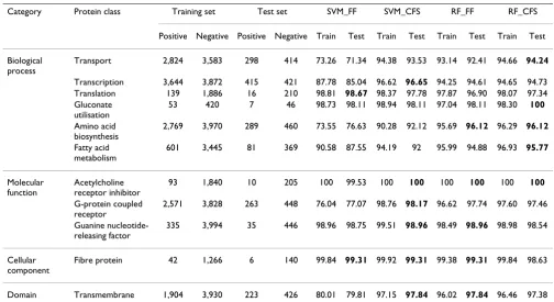
Table 5: Accuracy of predictions using training and blind test datasets with the SVM and random forest methods

Category Protein class Training set Test set SVM_FF SVM_CFS RF_FF RF_CFS

Positive Negative Positive Negative Train Test Train Test Train Test Train Test

Biological process

Transport 2,824 3,583 298 414 73.26 71.34 94.38 93.53 93.14 92.41 94.66 94.24

Transcription 3,644 3,872 415 421 87.78 85.04 96.62 96.65 94.25 94.61 94.65 94.73

Translation 139 1,886 16 210 98.81 98.67 98.37 97.78 97.87 96.90 98.07 97.34

Gluconate utilisation

53 420 7 46 98.73 98.11 98.94 98.11 97.04 98.11 98.30 100

Amino acid biosynthesis

2,769 3,970 289 460 73.55 76.63 90.28 92.12 95.69 96.12 96.29 96.12

Fatty acid metabolism

601 3,445 81 369 90.58 87.55 94.19 92 95.99 94.88 96.93 95.77

Molecular function

Acetylcholine receptor inhibitor

93 1,840 10 205 100 99.53 100 100 100 100 100 100

G-protein coupled receptor

2,571 3,828 263 448 76.04 77.07 98.76 98.17 96.62 97.74 97.60 97.46

Guanine nucleotide-releasing factor

335 3,994 35 446 98.96 98.75 99.51 98.96 98.49 98.96 98.98 98.54

Cellular component

Fibre protein 42 1,266 6 140 99.84 99.31 99.92 99.31 99.38 99.31 99.84 98.63

Domain Transmembrane 1,904 3,930 223 426 80.01 79.81 97.15 97.84 96.02 97.84 96.46 97.38

(9)

classification trees that each use several bootstrap samples of training data and a randomly selected subset of fea-tures. The basic random forest method, using unpruned decision trees, selects features at random at each decision node. The final classification is obtained by combining the results of the trees via voting.

To identify protein functions in this study, LibSVM [69,70] and random forests [68] (available at Weka [67]) were used as the classification algorithms. The type of SVM used was a C-SVC machine, and the kernel was a radial basis function (RBF). The cost parameter was set at 4 and the other parameters were fixed at the default val-ues. The cost parameter used in the training process was selected from {0.5, 1, 2, 4, 6, 8, 10, 12}. For the datasets used in this study, the RBF was found to provide the best results. In the random forest method without feature selection analysis, the number of trees was 10 and the number of features was 9. In the random forest method with feature selection analysis, the number of trees was 10 and the number of features was 6 or 7 because the number of features selected by the feature selection method was small.

Performance evaluation criteria

The following measures were used to assess the perform-ance of the classifiers used in this study: accuracy, sensitiv-ity, F-measure, Matthew's correlation coefficient (MCC) [71,72], and the area under the receiver operating charac-teristic curve (AUC) [42,71]. A trade-off between sensitiv-ity and specificsensitiv-ity was observed as the prediction threshold was varied. AUC is an effective means of com-paring the overall prediction performance of different methods because it provides a single measure of overall threshold-independent accuracy. An AUC and MCC of 1 indicate perfect prediction accuracy. These measures are defined as follows:

where TP is the number of true positives, FP is the number of false positives, TN is the number of true negatives, FN

is the number of false negatives, and recall is equivalent to the sensitivity [21,73]. The formula for the AUC of a clas-sifier is as follows:

where S₀= ∑r_i, r_iis the rank of the ith positive sample in the ranked list, n₀is the number of positive samples, and

n₁is the number of negative samples [74,75].

Results and discussion

Performance of the four classification methods

One of the goals of our experiment was to find a more dis-criminative and smaller feature set for specific function prediction, based solely on sequence-based features. Therefore, we initially gathered numerous features solely from the protein sequence. The features that were redun-dant or irrelevant were then removed by feature selection. After feature selection, the remaining number of features was small, while the accuracy of function classification was greater than that of the full-feature set. The selected features and the selection rates for the traditional features and our new features are listed in Tables 3 and 4.

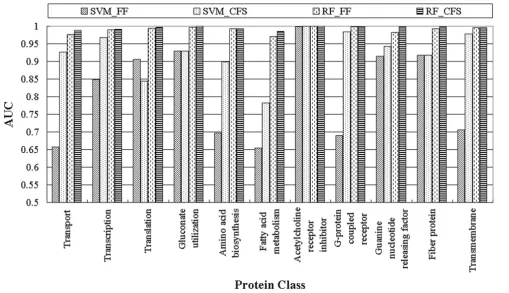
A summary of the performance of the four methods in classifying the 11 protein classes is provided in Table 5 and Figure 1. Among all the methods, SVM without fea-ture selection (SVM_FF) required more model-building time and had the lowest performance. However, this method did obtain the highest accuracy in two of the blind tests, for translation and fibre proteins (2 of the 11 protein classes).

SVM with feature selection (SVM_CFS) slightly outper-formed the random forest method with and without fea-ture selection (RF_CFS and RF_FF, respectively) and significantly outperformed SVM_FF. Given that more than one method had equal accuracy for some classes, the SVM_CFS method had the highest accuracy for classifying transcription, acetylcholine receptor inhibitor, G-protein coupled receptor, guanine nucleotide-releasing factor, fibre, and transmembrane proteins (6 of the 11 protein classes).

The random forest method without feature selection (RF_FF) had the highest accuracy for the following blind test sets: amino acid biosynthesis, acetylcholine receptor inhibitor, guanine nucleotide-releasing factor, fibre, and transmembrane proteins (5 of the 11 protein classes).

The random forest method with feature selection (RF_CFS) had the highest accuracy for classifying

trans-Accuracy TP TN

TP FN FP TN

= +

+ + + (8)

Sensitivity TP TP FN =

+ (9)

Specificity TN TN FP =

+ (10)

F measure precision recall precision recall

− = × ×

+ 2

(11)

MCC TP TN FP FN

TP FP TP FN TN FP TN FN

= × − ×

+ + + +

( ) ( )

( )( )( )( )

(12)

ˆ ( ) /

A S n n

n n = 0− 0 0 1+ 2

0 1

(10)

port, gluconate utilisation, amino acid biosynthesis, fatty acid metabolism, and acetylcholine receptor inhibitor proteins (5 of the 11 protein classes). Although both the RF_FF and RF_CFS methods had the highest accuracy for five protein classes, the performance of the RF_CFS method was better than that of the RF_FF method in terms of cost-effectiveness because a reduced-dimensional model was produced.

After careful analysis of the selected feature subsets and their performance in these experiments, the use of feature selection was found to improve classifier performance, as indicated in Table 5 and Figure 1. When comparing the SVM_FF and SVM_CFS methods, translation was the only protein class for which the SVM_FF method (AUC of 0.906, accuracy of 98.67) performed better than the SVM_CFS method (AUC of 0.844, accuracy of 97.78). For all the other classifications, the use of feature selection improved classifier performance. For classification of transport, transcription, amino acid biosynthesis, G-pro-tein coupled receptor, and transmembrane proG-pro-teins, both accuracy levels and AUCs significantly improved when feature selection was used. For example, the accuracy of transmembrane protein classification improved (79.81 to 97.84) and the AUC increased (0.706 to 0.978). In

addi-tion, the number of features used for classification was 35 of 484. For the G-protein coupled receptor, 39 of 484 fea-tures were included, and the accuracy of the classification was dramatically improved by feature selection (77.07 to 98.17), as was the AUC (0.69 to 0.984).

Although the accuracy of the random forest method was not significantly improved by feature selection, the AUC value for RF_CFS was slightly higher than that for RF_FF, except for the amino acid biosynthesis, acetylcholine receptor inhibitor, and G-protein coupled receptor classes. The larger the AUC, the better is the performance of the model. By comparing the AUCs averaged over all 11 protein classes, the RF_CFS method was found to outper-form the other methods (i.e. 0.995). Therefore, applying CFS to the dataset yielded improved performance and a more compact set of features.

For a more detailed evaluation of all the methods, several performance measures were applied. Detailed results for each method are presented in Tables 6, 7, 8, and 9, with a focus on sensitivity, specificity, F-measure, and MCC. The consistent performance of each method for predicting the protein functions of the 11 protein classes in both the 10-fold cross-validation test and the blind test demonstrates

Area under the ROC curves for the four methods for each protein class

Figure 1

(11)

the validity of our methods: SVM_FF, ± 3.0; SVM_CFS, ± 2.1; RF_FF ± 1.8; and RF_CFS, ± 1.2 (± refers to the differ-ence in accuracy between the training step and the blind test step). These results indicate that our models have good predictive power in discriminative testing processes.

Although good performance with the proposed new fea-tures was obtained using feature selection, we performed an additional experiment to demonstrate the usefulness of the proposed features in a clear and simple way, with-out relying on feature selection. The additional experi-ments were carried out using the 451 traditional features versus the 33 proposed features under the same condi-tions as the above experiments, and the performance of classification was compared (Tables 10 and 11). In the performance comparison with SVM, classification using only the 33 proposed features outperformed the 451 tra-ditional features for 5 of the 11 protein classes (transport, amino acid biosynthesis, fatty acid metabolism, G-protein coupled receptor, and transmembrane). In the perform-ance comparison with the random forest method, classifi-cation using only the 33 proposed features was superior or equal to use of the 451 traditional features for 4 of the 11

protein classes (translation, gluconate utilisation, fatty acid metabolism, and acetylcholine receptor inhibitor).

Meaningful features for protein function prediction The 451 traditional features used for prediction of protein function have been described in previous reports [17,22-24,28,32,36,37,43-45,76-78]. The present study intro-duces new features based on negatively and positively charged residues and analyses their utility. The average number of new features selected by CFS was 5.4 for the 11 protein classes. The raw dataset was analysed for the selected features, and three examples are provided in Fig-ures 2, 3, and 4.

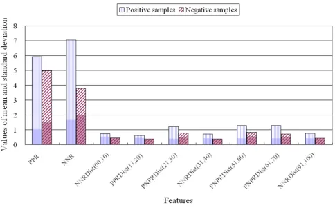
Figure 2 clearly demonstrates the differences in the means and standard deviations of the nine features used to clas-sify guanine nucleotide-releasing factor (the opaque col-our at the base of the bar graphs indicates the standard deviation). PPR and NNR for guanine nucleotide-releas-ing factor were higher than for the negative samples. For example, the NNR for guanine nucleotide-releasing factor was 7.04 (mean) ± 1.72 (standard deviation), while the NNR for the negative samples was 3.79 ± 2.0. It is worth

Table 6: Detailed results of SVM without feature selection (SVM_FF)

Protein class Sensitivity Specificity F-measure MCC

Transport 31.54 100 0.48 0.46

Transcription 71.08 98.81 0.83 0.73

Translation 81.25 100 0.90 0.9

Gluconate utilisation 85.71 100 0.92 0.92

Amino acid biosynthesis 39.45 100 0.57 0.53

Fatty acid metabolism 30.86 100 0.47 0.52

Acetylcholine receptor inhibitor 100 99.51 0.95 0.95

G-protein coupled receptor 38.02 100 0.55 0.53

Guanine nucleotide-releasing factor 82.86 100 0.91 0.9

Fibre protein 83.33 100 0.91 0.91

Transmembrane 41.26 100 0.58 0.56

MCC: Matthew's correlation coefficient

Table 7: Detailed results of SVM with feature selection (SVM_CFS)

Transport 87.58 97.83 0.92 0.87

Transcription 98.31 95.01 0.97 0.93

Translation 68.75 100 0.82 0.82

Amino acid biosynthesis 79.58 100 0.89 0.84

Fatty acid metabolism 56.79 99.73 0.72 0.71

Acetylcholine receptor inhibitor 100 100 1.00 1.00

G-protein coupled receptor 99.24 97.54 0.98 0.96

Guanine nucleotide-releasing factor 88.57 99.78 0.93 0.92

Fibre protein 83.33 100 0.91 0.91

Transmembrane 97.76 97.89 0.97 0.95

(12)

noting that negatively charged residues appear more fre-quently in the guanine nucleotide-releasing factor sequence than in those of other proteins. Furthermore, the NNR and PPR features are related to the number or percentage of negatively and positively charged residues, as these features were computed using a method based on charged residues. Because of this relationship, the mean percentages of positively charged residues and negatively charged residues were found to be similar to the PPR and NNR values, respectively. If the PPR for a specific protein family was high compared to that for other families, then the number of positively charged residues in that protein family was also higher than that in other families; simi-larly, if the NNR for a specific protein family was low, then the number of negatively charged residues in that protein family was also low. However, if the percentage of nega-tively charged residues was high and the NNR value was low, it is possible to infer that both negatively and posi-tively charged residues are present in the sequences, because NNR and PPR provide information on whether the two charged residue types co-exist in the sequence. The greater the difference between the percent negatively charged residues and the NNR, the more frequent is the

alternating occurrences of negatively and positively charged residues. For instance, golgi transport protein 1 [Swiss-Prot:Q9USJ2] consists of 129 amino acids with five negatively charged residues and eight positively charged residues. However, NNR and PPR were 0 and 2.32, respec-tively. This indicates that although the protein includes five negatively charged residues, the positively and nega-tively charged residues in the sequence always alternate among the neutral residues.

Previous studies in this field have analysed only the number or percentage of positively and negatively charged residues; however, the positions or regions of the charged residues in the sequence are very important in determining protein function and structure [79-82]. For example, Verma et al. [79] analysed a large panel of plaque-purified recovered viruses and demonstrated that the negatively charged residues at positions 440 and 441 were key residues that appeared to be involved in virus assembly. Therefore, although the total number of posi-tively and negaposi-tively charged residues is important, resi-dues in specific positions or local regions of the sequences are also important. Dist(x, y) for PPR, NNR, and PNPR pro-Table 8: Detailed results of the random forest method without feature selection (RF_FF)

Transport 87.58 95.89 0.84 0.91

Transcription 96.87 92.4 0.89 0.95

Translation 56.25 100 0.74 0.72

Amino acid biosynthesis 96.89 95.65 0.92 0.95

Fatty acid metabolism 71.6 100 0.82 0.84

Acetylcholine receptor inhibitor 100 100 1.00 1.00

Guanine nucleotide-releasing factor 85.71 100 0.92 0.92

Fibre protein 83.33 100 0.91 0.91

Transmembrane 95.07 99.3 0.95 0.97

MCC: Matthew's correlation coefficient

Table 9: Detailed results of the random forest method with feature selection (RF_CFS)

Transport 90.27 97.10 0.93 0.88

Transcription 96.63 92.87 0.95 0.90

Translation 62.50 100.00 0.77 0.78

Gluconate utilisation 100.00 100.00 1.00 1.00

Amino acid biosynthesis 95.85 96.30 0.95 0.92

Fatty acid metabolism 77.78 99.73 0.87 0.85

Acetylcholine receptor inhibitor 100.00 100.00 1.00 1.00

Guanine nucleotide-releasing factor 85.71 99.55 0.90 0.89

Fibre protein 66.67 100.00 0.80 0.81

Transmembrane 94.62 98.83 0.96 0.94

(13)

Table 10: Comparative performance of the novel feature set and traditional feature set using SVM

Protein class Novel feature set (33 features) Traditional feature set (451 features)

Training Accuracy

Test accuracy

Sensitivity Specificity AUC Training accuracy

Test accuracy Sensitivity Specificity AUC

Transport 75.0273 73.31 36.2 100 0.681 73.2636 72.19 33.6 100 0.668

Transcription 87.9723 88.15 99.3 77.2 0.882 92.5625 97.36 98.3 96.4 0.974

Translation 97.0864 97.34 62.5 100 0.813 98.8642 98.67 81.3 100 0.906

96.8288 96.22 71.4 100 0.857 98.7315 98.11 85.7 100 0.929

74.8627 77.83 42.6 100 0.713 73.5272 77.43 41.5 100 0.708

92.4123 90.22 45.7 100 0.728 90.5586 87.77 32.1 100 0.66

98.448 99.06 80 100 0.9 100 99.53 100 99.5 0.998

78.6998 80.87 48.3 100 0.741 76.1838 77.35 38.8 100 0.694

97.4359 97.92 77.1 99.6 0.883 98.8681 98.75 82.9 100 0.914

Fibre protein 96.789 95.89 0 100 0.5 99.8471 99.31 83.3 100 0.917

Transmembrane 85.2931 85.67 58.3 100 0.791 79.8937 80.58 43.5 100 0.717

AUC: Area under the curve.

Table 11: Comparative performance of the novel feature set and traditional feature set using the random forest

Protein class Novel feature set (33 features) Traditional feature set (451 features)

Training accuracy

Test accuracy

Sensitivity Specificity AUC Training accuracy

Test accuracy Sensitivity Specificity AUC

Transport 91.3688 90.30 86.6 93 0.968 92.9764 93.39 89.9 95.9 0.975

Transcription 90.9659 91.26 93.7 88.8 0.98 94.4252 95.33 96.4 94.3 0.99

Translation 97.679 97.78 68.8 100 0.95 98.0741 97.78 68.8 100 0.996

96.4059 98.11 85.7 100 0.997 97.2516 98.11 85.7 100 0.992

93.7676 94.52 91.7 96.3 0.983 94.836 95.46 94.8 95.9 0.991

95.7242 94.44 72.8 99.2 0.97 96.2926 94 69.1 99.5 0.964

99.6896 100 100 100 1 99.8965 100 100 100 1

94.4679 95.92 94.3 96.9 0.991 96.8745 97.18 94.7 98.7 0.993

96.7429 96.67 62.9 99.3 0.956 98.4985 97.92 74.3 99.8 0.992

Fibre protein 97.4771 95.89 33.3 98.6 0.798 99.2355 99.31 83.3 100 0.998

Transmembrane 93.555 93.52 87.4 96.7 0.978 95.9719 97.53 94.2 99.3 0.995

(14)

vides information on negatively and positively charged residues in local regions of the sequence. Seven features that provide local information were selected for classifica-tion of the guanine nucleotide-releasing factor. For exam-ple, PNPRDist_(61,70)was 1.29 ± 0.42 for the positive classification samples and 0.72 ± 0.53 for the negative samples. These findings indicate that alternating posi-tively and negaposi-tively charged residues occur more fre-quently in the local region from 61% to 70% in the guanine nucleotide-releasing factor sequence than in the negative protein samples. Therefore, local information on the distribution of negatively and positively charged resi-dues in the interval was informative. Because of these essential differences, guanine nucleotide-releasing factor proteins can be predicted with a high level of accuracy.

Figure 3 presents the results of analysis of the raw data for two features used in classifying transcription proteins.

PNPR for the positive classification samples was 12.04 ± 3.56, while for the negative samples, PNPR was 7.84 ± 3.03. These results indicate that continuous changes from a positively charged residue to the next negatively charged residue or vice versa occurred more frequently over the

full sequence of transcription proteins than in the nega-tive samples.

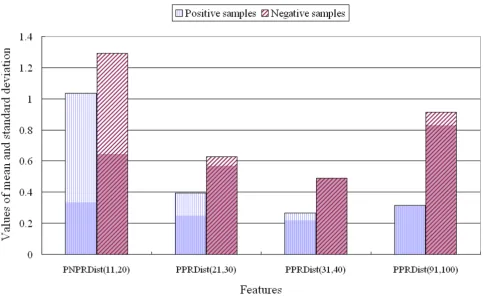
Figure 4 presents the results of analysis of the raw dataset for four features, when the proteins were classified using the random forest method. The mean values of the four selected features for gluconate utilisation were signifi-cantly lower than those of the negative samples. For exam-ple, PNPRDist_(11,20) for the gluconate utilisation sequences was 1.03 ± 0.3, while PNPRDist_(11,20)for the negative samples was 1.3 ± 0.6. These results indicate that there were fewer continuous changes from a positively charged residue to the next negatively charged residue or vice versa in the local region from 11% to 20% of the glu-conate utilisation sequences than in the negative samples.

There are two ways of using positively charged residues in classification and prediction of protein function. One process uses the positively charged residues arginine (R), histidine (H), and lysine (K) [20], while the other uses only arginine (R) and lysine (K) [24]. Although defining two groups of positively charged residues is potentially useful, we found that the use of arginine, histidine, and

Comparison of nine features used for classification of guanine nucleotide-releasing factor versus negative proteins

Figure 2

(15)

lysine achieved better results than did arginine and lysine. Specifically, the former (R, H, and K) was useful in classi-fying gluconate utilisation, fatty acid metabolism, G-pro-tein coupled receptor, transcription, and transport proteins, while the latter (R and K) was useful only in clas-sifying fibre proteins.

Significant findings

The following is a summary of the benchmark compari-sons and important findings of this study for prediction of protein function over a broad range of cellular compo-nents, molecular functions, and biological processes. Analyses were conducted by SVM and the random forest method with and without feature selection, based on many traditional and proposed features extracted from the sequences.

• Using a larger number of features to predict protein function does not always result in improved performance. In terms of accuracy and AUC, SVM with feature selection has distinct performance advantages with this type of data, indicating that removal of the many redundant and irrelevant features by feature selection can improve

pre-diction performance. However, there was no significant difference in prediction performance for the random for-est method with and without feature selection.

• The use of a particular classifier does not always result in improved performance. There is no single method that is optimal for all conditions because the performance of a method depends on the type of data involved, the size of the dataset, the number of features involved, the type of extracted features, and whether feature selection is used, among other things. Therefore, selection of the optimal classifier for a given dataset depends on an understanding of machine-learning algorithms, feature selection proc-esses, and biological background information relevant to the dataset.

• Features useful for predicting a specific protein function in a given dataset are not always useful for predicting another protein function – discriminative and informa-tive features differ according to protein function. There-fore, identifying discriminative features applicable to a broad range of protein classes is difficult.

Comparison of three features used for classification of transcription versus negative proteins

Figure 3

(16)

• Although many methods have recently been proposed for predicting protein function, most methods are not suitable for function prediction under high-throughput conditions, because they require information on protein structure. Currently, there is much more data available on protein sequences than on protein structures; thus, the methods developed in this study focused on predicting protein function based solely on features extracted from the protein sequence. This reduces the effort required to extract useful features, as the predictive or experimental work required to acquire structural information is both costly and time-consuming. In the experiments under-taken in this study, we found that sequence-based classifi-ers can also generate very good results.

• Local information regarding the protein sequence is meaningful in predicting protein function; several exam-ples have been presented to demonstrate its usefulness. Although identifying local information for a sequence is difficult and the information does not always correspond to striking difference in protein function, unique features extracted from specific positions or local regions can be predicted with a high level of accuracy.

• The numbers or percentages of positively and negatively charged residues are some of the most important and well-known features used for function prediction. PPR

and NNR were extracted from sequences based on the presence of negatively and positively charged residues. These novel features include information on the existence of negatively and positively charged residues as well as the manner in which the two charged residue types co-exist in a sequence. PPR and NNR were found to be selected more frequently for function prediction than were the number of negatively and positively charged residues. Thus, these features appear to be highly correlated with protein class and have a low inter-correlation with each other.

The above results indicate that it is possible to generate accurate predictions for a broad range of protein functions without the use of sequence or structural similarities. Fea-ture selection improves predictions for a variety of protein functions, but does not always ensure improved perform-ance, depending on the dataset and the method used. Finally, local information for protein sequences is mean-ingful for predicting protein function, and a feature set with good performance and dimensional reduction was

Comparison of local information used for classification of gluconate utilisation versus negative proteins

Figure 4

(17)

identified, as many features initially included in this study were removed by CFS.

Conclusion

Many previous studies have attempted to biologically and computationally determine meaningful and accurate fea-tures that assist in predicting protein function. Feafea-tures that show an obvious propensity for predicting many dif-ferent protein functions have not yet been reported, and this provides a motivation for discovering the relationship between features and protein function.

This paper described a highly accurate prediction method capable of identifying protein function by using features extracted solely from protein sequences, irrespective of sequence and structural similarities. In this study, the PPR,

NNR, PNPR, and Dist₍_x_,_y₎features were introduced. In pre-dicting the functions of 11 different proteins, a high per-formance (94.23–100%) was achieved and predictive features for several protein classes were effectively identi-fied.

The results presented here suggest that our new features, developed in the course of this study, will be useful in dicting many protein class functions. We believe that pre-diction performance can be improved by combining sequence-based features and additional features, such as predicted secondary structure, surface area, and subcellu-lar location. Accordingly, further insight into feature anal-ysis and biological understanding is needed. In future studies, we will apply this method to predict the functions of proteins that have not been identified by sequence alignment.

Competing interests

The authors declare that they have no competing interests.

Authors' contributions

BJL conducted the experiments and analysis, conceived the concepts of PPR, NNR, PNPR, and Dist₍_x_,_y₎, and wrote the manuscript. MSS and YJO assisted in developing the method and revising the manuscript. KHR and HSO supervised the work, provided useful suggestions to improve performance, and revised the manuscript. All authors read and approved the manuscript.

Acknowledgements

This work was supported by a grant from the Korean Ministry of Education, Science, and Technology (The Regional Core Research Programme/Chung-buk BIT Research-Oriented University Consortium) and by Basic Science Research Program through the National Research Foundation of Korea (NRF)funded by the Ministry of Education, Science and Technology (MEST) (R01-2007-000-10926-0, R11-2008-014-02002-0).

References

1. Altschul SF, Gish W, Miller W, Myers EW, Lipman DJ: Basic local alignment search tool. J Mol Biol 1990, 215:403-410.

2. Altschul SF, Madden TL, Schaffer AA, Zhang J, Zhang Z, Miller W, Lip-man DJ: Gapped BLAST and PSI-BLAST: a new generation of protein database search programs. Nucleic Acids Res 1997, 35:3389-3402.

3. Pearson WR, Lipman DJ: Improved tools for biological sequence comparison. Proc Natl Acad Sci USA 1988, 85:2444-2448. 4. Benner SA, Chamberlin SG, Liberles DA, Govindarajan S, Knecht L:

Functional inferences from reconstructed evolutionary biol-ogy involving rectified databases – an evolutionarily grounded approach to functional genomics. Res Microbiol 2000, 151:97-106.

5. Cai CZ, Han LY, Ji ZL, Chen X, Chen YZ: Enzyme family classifi-cation by support vector machines. Proteins 2004, 55:66-76. 6. Dobson PD, Doig AJ: Predicting enzyme class from protein

structure without alignments. J Mol Biol 2005, 345:187-199. 7. Han LY, Cai CZ, Ji ZL, Cao ZW, Cui J, Chen YZ: Predicting

func-tional family of novel enzymes irrespective of sequence sim-ilarity: a statistical learning approach. Nucleic Acids Res 2004, 32:6437-6444.

8. Wang X, Schroeder D, Dobbs D, Honavar V: Automated data-driven discovery of motif-based protein function classifiers.

Inf Sci 2003, 155:1-18.

9. Lapinsh M, Gutcaits A, Prusis P, Post C, Lundstedt T, Wikberg JES: Classification of G-protein coupled receptors by alignment-independent extraction of principal chemical properties of primary amino acid sequences. Protein Sci 2002, 11:795-805. 10. Rost B: Twilight zone of protein sequence alignments. Protein

Eng 1999, 12:85-94.

11. Hobohm U, Sander C: A sequence property approach to searching protein databases. J Mol Biol 1995, 251:390-399. 12. Claeyssens M, Henrissat B: Specificity mapping of cellulolytic

enzymes: classification into families of structurally related proteins confirmed by biochemical analysis. Protein Sci 1992, 1:1293-1297.

13. Karp PD: What we do not know about sequence analysis and sequence database. Bioinformatics 1998, 14:753-754.

14. Hawkins T, Kihara D: Function prediction of uncharacterized proteins. J Bioinform Comput Biol 2007, 5:1-30.

15. Holm L, Sander C: Dali: a network tool for protein structure comparison. Trends Biochem Sci 1995, 20:478-480.

16. Kawabata T: MATRAS: a program for protein 3D structure comparison. Nucleic Acids Res 2003, 31:3367-3369.

17. Eidhammer I, Jonassen I, Taylor WR: Protein structure compari-son and structure patterns. J Comput Biol 2000, 7:685-716. 18. Friedberg I: Automated protein function prediction-the

genomic challenge. Brief Bioinformatics 2006, 7:225-242. 19. Russell RB, Saqi MA, Bates PA, Sayle RA, Sternberg MJ: Recognition

of analogous and homologous protein folds – assessment of prediction success and associated alignment accuracy using empirical substitution matrices. Protein Eng 1998, 11:1-9. 20. Syed U, Yona G: Enzyme function prediction with

interpreta-ble models. In Computational Systems Biology Edited by: Samudrala R, McDermott J, Bumgarner R. New York: Humana Press; 2007:1-33. 21. Borro LC, Oliveira SRM, Yamagishi MEB, Mancini AL, Jardine JG,

Maz-oni I, Santos EHD, Higa RH, Kuser PR, Neshich G: Predicting enzyme class from protein structure using Bayesian classifi-cation. Genet Mol Res 2006, 5:193-202.

22. Cai CZ, Han LY, Ji ZL, Chen X, Chen YZ: SVM-Prot: web-based support vector machine software for functional classification of a protein from its primary sequence. Nucleic Acids Res 2003, 31:3692-3697.

23. Jensen LJ, Gupta R, Blom N, Devos D, Tamames J, Kesmir C, Nielsen H, Stærfeldt HH, Rapacki K, Workman C, Andersen CAF, Knudsen S, Krogh A, Valencia A, Brunak S: Prediction of human protein function from post-translational modifications and localiza-tion features. J Mol Biol 2002, 319:1257-1265.