S O F T W A R E
Open Access
joineRML: a joint model and software
package for time-to-event and multivariate
longitudinal outcomes
Graeme L. Hickey
1, Pete Philipson
2, Andrea Jorgensen
1and Ruwanthi Kolamunnage-Dona
1*Abstract
Background: Joint modelling of longitudinal and time-to-event outcomes has received considerable attention over recent years. Commensurate with this has been a rise in statistical software options for fitting these models. However, these tools have generally been limited to a single longitudinal outcome. Here, we describe the classical joint model to the case ofmultiplelongitudinal outcomes, propose a practical algorithm for fitting the models, and demonstrate how to fit the models using a new package for the statistical software platform R,joineRML.
Results: A multivariate linear mixed sub-model is specified for the longitudinal outcomes, and a Cox proportional hazards regression model with time-varying covariates is specified for the event time sub-model. The association between models is captured through a zero-mean multivariate latent Gaussian process. The models are fitted using a Monte Carlo Expectation-Maximisation algorithm, and inferences are based on approximate standard errors from the empirical profile information matrix, which are contrasted to an alternative bootstrap estimation approach. We illustrate the model and software on a real data example for patients with primary biliary cirrhosis with three repeatedly measured biomarkers.
Conclusions: An open-source software package capable of fitting multivariate joint models is available. The underlying algorithm and source code makes use of several methods to increase computational speed.
Keywords: Joint modelling, Longitudinal data, Multivariate data, Time-to-event data, Software
Background
In many clinical studies, subjects are followed-up repeat-edly and response data collected. For example, routine blood tests might be performed at each follow-up clinic appointment for patients enrolled in a randomized drug trial, and biomarker measurements recorded. An event time is also usually of interest, for example time of death or study drop-out. It has been repeatedly shown else-where that if the longitudinal and event-time outcomes are correlated, then modelling the two outcome processes separately, for example using linear mixed models and Cox regression models, can lead to biased effect size esti-mates [1]. The same criticism has also been levelled at the
*Correspondence:[email protected]
1Department of Biostatistics, Institute of Translational Medicine, University of Liverpool, Waterhouse Building, 1-5 Brownlow Street, L69 3GL Liverpool, UK Full list of author information is available at the end of the article
application of so-called two-stage models [2]. The motiva-tion for using joint models can be broadly separated into interest in drawing inference about (1) the time-to-event process whilst adjusting for the intermittently measured (and potentially error-prone) longitudinal outcomes, and (2) the longitudinal data process whilst adjusting for a potentially informative drop-out mechanism [3]. The lit-erature on joint modelling is extensive, with excellent reviews given by Tsiatis and Davidian [4], Gould et al. [5], and the book by Rizopoulos [6].
Joint modelling has until recently been predominated by modelling a single longitudinal outcome together with a solitary event time outcome; herein referred to as univariate joint modelling. Commensurate with method-ological research has been an increase in wide-ranging clinical applications (e.g. [7]). Recent innovations in the field of joint models have included the incorporation of multivariate longitudinal data [8], competing risks data
[9, 10], recurrent events data [11], multivariate time-to-event data [12, 13], non-continuous repeated measure-ments (e.g. count, binary, ordinal, and censored data) [14], non-normally and non-parametrically distributed random effects [15], alternative estimation methodolo-gies (e.g. Bayesian fitting and conditional estimating equations) [16, 17], and different association structures [18]. In this article, we specifically focus on the first inno-vation: multivariate longitudinal data. In this situation, we assume that multiple longitudinal outcomes are measured on each subject, which can be unbalanced and measured at different times for each subject.
Despite the inherently obvious benefits of harnessing all data in a single model or the published research on the topic of joint models for multivariate longitu-dinal data, a recent literature review by Hickey et al. [19] identified that publicly available software for fitting such models was lacking, which has translated into lim-ited uptake by biomedical researchers. In this article we present the classical joint model described by Henderson et al. [3] extended to the case of multiple longitudi-nal outcomes. An algorithm proposed by Lin et al. [20] is used to fit the model, augmented by techniques to reduce the computational fitting time, including a quasi-Newton update approach, variance reduction method, and dynamic Monte Carlo updates. This algorithm is encoded into a R sofware package–joineRML. A sim-ulation analysis and real-world data example are used to demonstrate the accuracy of the algorithm and the software, respectively.
Implementation
As a prelude to the introduction and demonstration of the newly introduced software package, in the following section we describe the underlying model formulation and model fitting methodology.
Model
For each subject i = 1,. . .,n, yi = yi1,. . .,yiK is the K-variate continuous outcome vector, where each yik denotes an (nik × 1)-vector of observed
longitudi-nal measurements for the k-th outcome type: yik =
(yi1k,. . .,yinikk)
. Each outcome is measured at observed
(possibly pre-specified) timestijkforj=1,. . .,nik, which can differ between subjects and outcomes. Additionally, for each subject there is an event time Ti∗, which is subject to right censoring. Therefore, we observe Ti = min(Ti∗,Ci), whereCicorresponds to a potential censor-ing time, and the failure indicatorδi, which is equal to 1 if the failure is observed(Ti∗ ≤ Ci)and 0 otherwise. We assume that both censoring and measurement times are non-informative.
The model we describe is the natural extension of the
model proposed by Henderson et al. [3] to the case
of multivariate longitudinal data. The model posits an unobserved or latent zero-mean (K + 1)-variate Gaus-sian process that is realised independently for each sub-ject,Wi(t) =
W1(1i)(t),. . .,W1(K)i (t),W2i(t)
. This latent process subsequently links the separate sub-models via association parameters.
Thek-th longitudinal data sub-model is given by
yik(t)=μik(t)+W1(k)i (t)+εik(t), (1)
whereμik(t)is the mean response, andεik(t)is the model error term, which we assume to be independent and iden-tically distributed normal with mean 0 and variance σk2. The mean response is specified as a linear model
μik(t)=xik(t)βk, (2) where xik(t) is a pk-vector of (possibly) time-varying covariates with corresponding fixed effect terms βk. W1(k)i (t)is specified as
W1(k)i (t)=zik(t)bik, (3)
where zik(t) is an rk-vector of (possibly) time-varying
covariates with corresponding subject-and-outcome
random effect terms bik, which follow a zero-mean
multivariate normal distribution with(rk×rk)
-variance-covariance matrix Dkk. To account for dependence
between the different longitudinal outcome outcomes, we let cov(bik,bil)= Dklfork=l. Furthermore, we assume
εik(t) and bik are uncorrelated, and that the censoring times are independent of the random effects. These distributional assumptions together with the model given by (1)–(3) are equivalent to the multivariate extension of the Laird and Ware [21] linear mixed effects model. More flexible specifications ofW1(k)i (t) can be used [3], including for example, stationary Gaussian processes. However, we do not consider these cases here owing to the increased computational burden it carries, even for the univariate case.
The sub-model for the time-to-event outcome is given by the hazard model
λi(t)=λ0(t)exp
vi (t)γv+W2i(t)
,
whereλ0(·)is an unspecified baseline hazard, andvi(t)is aq-vector of (possibly) time-varying covariates with cor-responding fixed effect terms γv. Conditional on Wi(t) and the observed covariate data, the longitudinal and time-to-event data generating processes are conditionally independent. To establish a latent association, we specify W2i(t)as a linear combination of
W1(1i)(t),. . .,W1(K)i (t)
:
W2i(t)= K
k=1
whereγy=(γy1,. . .,γyK)are the corresponding associa-tion parameters. To emphasise the dependence ofW2i(t) on the random effects, we explicitly write it asW2i(t,bi) from here onwards. As perW1(k)i (t),W2i(t,bi)can also be flexibly extended, for example to include subject-specific frailty effects [3].
Estimation
Likelihood
For each subjecti, letXi=Kk=1XikandZi=Kk=1Zik be block-diagonal matrices, whereXik =
xi1k,. . .,xin ikk is an(nik ×pk)-design matrix, with the j-th row corre-sponding to thepk-vector of covariates measured at time tijk, anddenotes the direct matrix sum. The notation similarly follows for the random effects design matrices, Zik. We denote the error terms by a diagonal matrixi=
K
k=1σk2Inik and write the overall variance-covariance matrix for the random effects as
D=
⎛ ⎜ ⎝
D11 · · · D1K ..
. . .. ... D1K · · · DKK
⎞ ⎟ ⎠,
where In denotes ann× n identity matrix. We further
define β = β1,. . .,βK and bi =
bi1,. . .,biK . Hence, we can then rewrite the longitudinal outcome sub-model as
yi|bi,β,i ∼ N(Xiβ+Zibi,i), withbi|D ∼ N(0,D).
For the estimation, we will assume that the covariates in the time-to-event sub-model are time-independent and known at baseline, i.e.vi ≡ vi(0). Extensions of the esti-mation procedure for time-varying covariates are outlined elsewhere [6, p. 115]. Theobserveddata likelihood for the joint outcome is given by
n
i=1
∞
−∞f(yi|bi,θ)f(Ti,δi|bi,θ)f(bi|θ)dbi
, (4)
whereθ =
β, vech(D),σ12,. . .,σK2,λ0(t),γv,γy is the collection of unknown parameters that we want to esti-mate, with vech(D)denoting the half-vectorisation opera-tor that returns the vecopera-tor of lower-triangular elements of matrixD.
As noted by Henderson et al. [3], the observed data likelihood can be calculated by rewriting it as
n
i=1 f(yi|θ)
∞
−∞f(Ti,δi|bi,θ)f(bi|yi,θ)dbi
,
where the marginal distributionf(yi|θ)is a multivariate normal density with meanXiβ and variance-covariance matrixi+ZiDZi , andf(bi|yi,θ)is given by (6).
MCEM algorithm
We determine maximum likelihood estimates of the parametersθusing the Monte Carlo Expectation Maximi-sation (MCEM) algorithm [22], by treating the random effectsbias missing data. This is effectively the same as the conventional Expectation-Maximisation (EM) algo-rithm, as used by Wulfsohn and Tsiatis [23] and Ratcliffe et al. [24] in the context of fitting univariate data joint models, except the E-step exploits a Monte Carlo (MC) integration routine as opposed to Gaussian quadrature methods, which we expect to be beneficial when the dimension of random effects becomes large.
Starting from an initial estimate of the parameters,θˆ(0), the procedure involves iterating between the following two steps until convergence is achieved.
1. E-step. At the(m+1)-th iteration, we compute the
expected log-likelihood of thecomplete data
conditional on theobserved data and the current
estimate of the parameters,
Q(θ| ˆθ(m))= n
i=1
Elogf(yi,Ti,δi,bi|θ)
= n
i=1 ∞
−∞
logf(yi,Ti,δi,bi|θ)
f(bi|Ti,δi,yi;θˆ (m)
)dbi.
Here, the complete-data likelihood contribution for
subjecti is given by the integrand of (4).
2. M-step. We maximiseQ(θ| ˆθ(m))with respect toθ.
Namely, we set
ˆ
θ(m+1)=argmax
θ Q
θ| ˆθ(m) .
The M-step estimators naturally follow from Wulfsohn and Tsiatis [23] and Lin et al. [20]. Maximizers for all parameters exceptγvandγyare available in closed-form; algebraic details are presented in Additional file 1. The parametersγ = (γv,γy)are jointly updated using a
one-step Newton-Raphson algorithm as
ˆ
γ(m+1)= ˆγ(m)+Iγˆ(m) −1Sγˆ(m) ,
where γˆ(m) denotes the value of γ at the current itera-tion,S
ˆ
γ(m) is the corresponding score, andI
ˆ γ(m) is the observed information matrix, which is equal to the derivative of the negative score. Further details of this update are given in Additional file1. The M-step forγ is computationally expensive to evaluate. Therefore, we also propose a quasi-Newton one-step update by approx-imatingI
ˆ
γ(m) by an empirical information matrix for
0.5 rather than 1, which is used when using the Newton-Raphson update.
The M-step involves terms of the form E
h(bi)|Ti,
δi,yi;θˆ
, for known functionsh(·). The conditional expecta-tion of a funcexpecta-tion of the random effects can be written as
Eh(bi)|Ti,δi,yi;θˆ
=
∞
−∞h(bi)f(bi|yi;θˆ)f(Ti,δi|bi;θˆ)dbi ∞
−∞f(bi|yi;θˆ)f(Ti,δi|bi;θˆ)dbi ,
(5)
wheref(Ti,δi|bi;θˆ)is given by
f(Ti,δi|bi;θ)=
λ0(Ti)expvi γv+W2i(Ti,bi)
δi
×exp
− Ti
0 λ0(
u)expvi γv+W2i(u,bi)
du
and f(bi|yi;θˆ) is calculated from multivariate normal distribution theory as
bi|yi,θ ∼N
Ai
Zi −i1(yi−Xiβ)
,Ai , (6)
withAi =
Zi −i 1Zi+D−1
−1
. As this becomes putationally expensive using Gaussian quadrature com-mensurate with increasing dimension ofbi, we estimate the integrals by MC sampling such that the expectation is approximated by the ratio of the sample means for h(bi)f(Ti,δi|bi;θˆ) and f(Ti,δi|bi;θˆ) evaluated at each MC draw. Furthermore, we use antithetic simulation for variance reduction in the MC integration. Instead of directly sampling from (6), we sample ∼ N(0,Ir)and obtain thepairs
Ai
Zi −i 1(yi−Xiβ)
±Ci,
whereCi is the Cholesky decomposition ofAi such that CiCi =Ai. Therefore we only need to drawN/2 samples using this approach, and by virtue of the negative correla-tion between the pairs, it leads to a smaller variance in the sample means taken in the approximation than would be obtained fromNindependent simulations. The choice of Nis described below.
Initial values
The EM algorithm requires that initial parameters are specified, namely θˆ(0). By choosing values close to the maximizer, the number of iterations required to reach convergence should be reduced.
For the time-to-event sub-model, a quasi-two-stage model is fitted when the measurement times are balanced, i.e. whentijk = tij∀k. That is, we fitseparateLMMs for each longitudinal outcome as per (1), ignoring the cor-relation between different outcomes. This is straightfor-ward to implement using standard software, in particular
usinglme()andcoxph()from the R packagesnlme
[26] and survival [27], respectively. From the fitted models, the best linear unbiased predictions (BLUPs) of the separate model random effects are used to estimate eachW1(k)i (t)function. These estimates are then included as time-varying covariates in a Cox regression model, alongside any other fixed effect covariates, which can be straightforwardly fitted using standard software. In the situation that the data are not balanced, i.e. whentijk=tij
∀k, then we fit a standard Cox proportional hazards regression model to estimateγvand setγyk=0∀k.
For the longitudinal data sub-model, when K>1
we first find the maximum likelihood estimate of
β, vech(D),σ12,. . .,σK2by running a separate EM algo-rithm for the multivariate linear mixed model. Both the E- and M-step updates are available in closed form, and the initial parameters for this EM algorithm are available from the separate LMM fits, withDinitialized as block-diagonal. As these are estimated using an EM rather than MCEM algorithm, we can specify a stricter convergence criterion on the estimates.
Convergence and stopping rules
Two standard stopping rules for the deterministic EM algorithm used to declare convergence are the relative and absolute differences, defined as
(m+1)
rel = max
⎧ ⎪ ⎨ ⎪ ⎩
θˆ(m+1)− ˆθ(m)
θˆ(m)+1
⎫ ⎪ ⎬ ⎪
⎭< 0, and (7)
(m+1)
abs = maxθˆ
(m+1)
− ˆθ(m)< 2 (8)
respectively, for some appropriate choice of 0, 1, and
2, where the maximum is taken over the components
of θ. For reference, the R package JM[28] implements (7) (in combination with another rule based on relative change in the likelihood), whereas the R packagejoineR [29] implements (8). The relative difference might be unstable about parameters near zero that are subject to MC error. Therefore, the convergence criterion for each parameter might be chosen separately at each EM itera-tion based on whether the absolute magnitude is below or above some threshold. A similar approach is adopted in the EM algorithms employed by the software package SAS [30, p. 330].
The choice of N and the monitoring of convergence
will be swamped by MC error. Therefore, it has been
rec-ommended that one increase N as the estimate moves
towards the maximizer. Although this might be done sub-jectively [31] or by pre-specified rules [32], an automated approach is preferable and necessary for a software imple-mentation. Booth and Hobert [33] proposed an update rule based on a confidence ellipsoid for the maximizer at the(m+1)-th iteration, calculated using an approximate sandwich estimator for the maximizer, which accounts for the MC error at each iteration. This approach requires additional variance estimation at each iteration, therefore we opt for a simpler approach described by Ripatti et al. [34]. Namely, we calculate a coefficient of variation at the
(m+1)-th iteration as
cv
(m+1)
rel =
sd(mrel−1),(m)rel ,(mrel+1) mean(mrel−1),(m)rel ,(mrel+1)
,
where(mrel+1)is given by (7), and sd(·)and mean(·)are the sample standard deviation and mean functions, respec-tively. If cv
(m+1)
rel >cv
(m)rel , thenN:=N+ N/δ, for some small positive integerδ. Typically, we run the
MCEM algorithm with a small N (for a fixed number
of iterations—aburn-in) before implementing this update rule in order to get into the approximately correct param-eter region. Appropriate values for other paramparam-eters will be application specific, however we have found δ = 3, N =100K(for 100Kburn-in iterations),1 =0.001, and
0=2=0.005 delivers reasonably accurate estimates in many cases, whereKwas earlier defined as the number of longitudinal outcomes.
As the EM monotonicity property is lost due to the MC integrations in the MCEM algorithm, convergence might be prematurely declared due to stochasticity if the
-values are too large. To reduce the chance of this occur-ring, we require that the stopping rule is satisfied for 3 consecutive iterations [33, 34]. However, in any case, trace plots should be inspected to confirm convergence is appropriate.
Standard error estimation
Standard error (SE) estimation is usually based on invert-ing the observed information matrix. When the baseline hazard is unspecified, as is the case here, this presents several challenges. First, λˆ0(t) will generally be a high-dimensional vector, which might lead to numerical diffi-culties in the inversion of the observed information matrix [6]. Second, the profile likelihood estimates based on the usual observed information matrix approach are known to be underestimated [35]. The reason for this is that the profile estimates are implicit, since the posterior expec-tations, given by (5), depend on the parameters being estimated, includingλ0(t)[6, p. 67].
To overcome these challenges, Hsieh et al. [35] rec-ommended to use bootstrap methods to calculate the SEs. However, this approach is computationally expensive. Moreover, despite the purported theoretical advantages, we also note that recently it has been suggested that boot-strap estimators might actuallyoverestimatethe SEs; e.g. [36, p. 740] and [35, p. 1041]. At the model develop-ment stage, it is often of interest to gauge the strength of association of model covariates, which is not feasi-ble with repeated bootstrap implementations. Hence, an approximate SE estimator is desirable. In either case, the theoretical properties will be contaminated by the addi-tion of MC error from the MCEM algorithm, and it is not yet fully understood what the ramifications of this are. Hence, any standard errors must be interpreted with a degree of caution. We consider two estimators below.
1. Bootstrap method. These are estimated by sam-pling n subjects with replacement and re-labelling the subjects with indices i = 1,. . .,n. We then re-fit the model to the bootstrap-sampled dataset. It is important to note that we re-sample subjects, not individual data points. This is repeated B-times, for a sufficiently large integerB. Since we already have the MLEs from the fitted model, we can use these as initial values for each boot-strap model fit, thus reducing initial computational over-heads in calculating approximate initial parameters. For each iteration, we extract the model parameter estimates for β, vech(D),σ12,. . .,σK2,γv,γy . Note that we do not estimate SEs forλ0(t)using this approach. However, they are generally not of inferential interest. When Bis sufficiently large, the SEs can be estimated from the esti-mated coefficients of the bootstrap samples. Alternatively, 100(1−α)%-confidence intervals can be estimated from the the 100α/2-th and 100(1−α/2)-th percentiles.
2. Empirical information matrix method.Using the Breslow estimator for0tλ0(u)du, the profile score vector forθ−λ=(β, vech(D),σ12,. . .,σK2,γ)is calculated (see Additional file 1). We approximate the profile informa-tion forθ−λbyIe−1/2(θˆ−λ0), whereIe(θ−λ0)is the observed empirical information [25] given by
Ie(θ−λ)= n
i=1
si(θ−λ)⊗2− 1 nS(θ−λ)
⊗2, (9)
to the exact same theoretical limitation of underestima-tion described by Hsieh et al. [35], since the profiling was implicit; that is, because the posterior expectations involve the parametersθ.
Software
The model described here is implemented in the R
packagejoineRML, which is available on the The
Com-prehensive R Archive Network (CRAN) (https://CRAN.
R-project.org/package=joineRML). The principal
func-tion injoineRMLismjoint(). The primary arguments
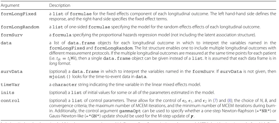
for implementingmjoint()are summarised in Table1. To achieve computationally efficiency, parts of the MCEM
algorithm in joineRML are coded in C++ using the
Armadillo linear algebra library and integrated using the
R packageRcppArmadillo[37].
A model fitted using themjoint() function returns
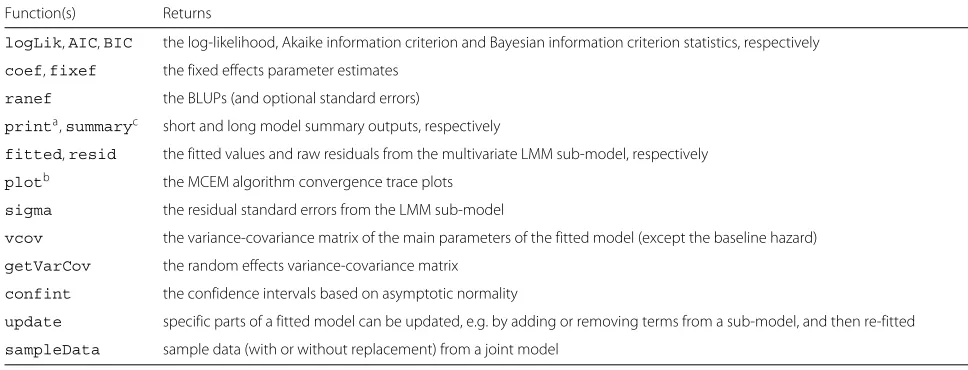
an object of class mjoint. By default, approximate SE estimates are calculated using the empirical information matrix. If one wishes to use bootstrap standard error esti-mates, then the user can pass the model object to the bootSE()function. Several generic functions (or rather, S3 methods) can also be applied to mjointobjects, as described in Table 2. These generic functions include
common methods, for examplecoef(), which extracts
the model coefficients; ranef(), which extracts the
BLUPs (and optional standard errors); and resid(),
which extracts the residuals from the linear mixed sub-model. The intention of these functions is to have a common syntax with standard R packages for linear mixed
models [26] and survival analysis [27]. Additionally, plot-ting capabilities are included injoineRML. These include trace plots for assessment of convergence of the MCEM algorithm, and caterpillar plots for subject-specific ran-dom effects (Table2).
The package also provides several datasets, and a func-tion simData() that allows for simulation of data from joint models with multiple longitudinal outcomes. joineRMLcan also fit univariate joint models, however in this case we would currently recommend that the R packagesjoineR[29],JM[28], orfrailtypack[38] are used, which are optimized for the univariate case and exploits Gaussian quadrature. In addition, these packages allow for extensions to more complex cases; for example, competing risks [28,29] and recurrent events [38].
Results
Simulation analysis
A simulation study was conducted assuming two longitu-dinal outcomes andn = 200 subjects. Longitudinal data were simulated according to a follow-up schedule of 6 time points (at times 0, 1,. . ., 5), with each model includ-ing subject-and-outcome-specific random-intercepts and random-slopes: bi = (b0i1,b1i1,b0i2,b1i2), Correlation was induced between the 2 outcomes by assuming cor-relation of−0.5 between the random intercepts for each outcome. Event times were simulated from a Gompertz distribution with shapeθ1 = −3.5 and scale exp(θ0) = exp(0.25) ≈ 1.28, following the methodology described by Austin [39]. Independent censoring times were drawn
Table 1The primary argumentsawith descriptions for themjoint()function in the R packagejoineRML
Argument Description
formLongFixed alistofformulaefor the fixed effects component of each longitudinal outcome. The left hand-hand side defines the
response, and the right-hand side specifies the fixed effect terms.
formLongRandom alistof one-sidedformulaespecifying the model for the random effects effects of each longitudinal outcome.
formSurv aformulaspecifying the proportional hazards regression model (not including the latent association structure).
data a list of data.frame objects for each longitudinal outcome in which to interpret the variables named in the
formLongFixedandformLongRandom. The list structure enables one to include multiple longitudinal outcomes with
different measurement protocols. If the multiple longitudinal outcomes are measured at the same time points for each patient (i.e.tijk=tij∀k), then a singledata.frameobject can be given instead of alist. It is assumed that each data frame is in
long format.
survData (optional) adata.framein which to interpret the variables named in theformSurv. IfsurvDatais not given, then
mjoint()looks for the time-to-event data indata.
timeVar acharacterstring indicating the time variable in the linear mixed effects model.
inits (optional) alistof initial values for some or all of the parameters estimated in the model.
control (optional) alistof control parameters. These allow for the control of0,1, and2in (7) and (8); the choice ofN,δ, and
convergence criteria; the maximum number of MCEM iterations, and the minimum number of MCEM iterations during burn-in. Additionally, the control argumentgammaOptcan be used to specify whether a one-step Newton-Raphson (="NR") or Gauss-Newton-like (="GN") update should be used for the M-step update ofγ.
amjoint()also takes the optional additional argumentsverbose, which ifTRUEallows for monitoring updates at each MCEM algorithm iteration, andpfs, which if
FALSEcan force the function not to calculate post-fit statistics such as the BLUPs and associated standard errors of the random effects and approximate standard errors of
Table 2Additional functions with descriptions that can be applied to objects of classmjointa
Function(s) Returns
logLik,AIC,BIC the log-likelihood, Akaike information criterion and Bayesian information criterion statistics, respectively
coef,fixef the fixed effects parameter estimates
ranef the BLUPs (and optional standard errors)
printa,summaryc short and long model summary outputs, respectively
fitted,resid the fitted values and raw residuals from the multivariate LMM sub-model, respectively
plotb the MCEM algorithm convergence trace plots
sigma the residual standard errors from the LMM sub-model
vcov the variance-covariance matrix of the main parameters of the fitted model (except the baseline hazard)
getVarCov the random effects variance-covariance matrix
confint the confidence intervals based on asymptotic normality
update specific parts of a fitted model can be updated, e.g. by adding or removing terms from a sub-model, and then re-fitted
sampleData sample data (with or without replacement) from a joint model
aprint()also applies to objects of classsummary.mjointandbootSEinheriting from thesummary()andbootSE()functions, respectively
bplot()also accepts objects of classranef.mjointinheriting from theranef()function, which displays a caterpillar plot (with 95% prediction intervals) for each
random effect
csummary()can also take the optional argument of an object of classbootSEinheriting from the functionbootSE(), which overrides the approximate SEs and CIs with
those from a bootstrap estimation routine
from an exponential distribution with rate 0.05. Any sub-ject where the event and censoring time exceeded 5 was administratively censored at the truncation timeC=5.1. For all sub-models, we included a pair of covariatesXi =
(xi1,xi2), where xi1 is a continuous covariate indepen-dently drawn fromN(0, 1) and xi2 is a binary covariate independently drawn from Bin(1, 0.5). The sub-models are given as
yijk = (β0,k+bi0k)+(β1,k+bi1k)tj
+ β2,kxi1+β3,kxi2+εijk, fork=1, 2;
λi(t) = exp{(θ0+θ1t)+γv1xi1+γv2xi2
+ γy1(bi01+bi11t)+γy2(bi02+bi12t)
; bi ∼ N4(0,D);
εijk ∼ N(0,σk2),
where D is specified unstructured (4 × 4)-covariance matrix with 10 unique parameters. Simulating datasets is
straightforward using thejoineRML package by means
of thesimData()function. The true parameter values
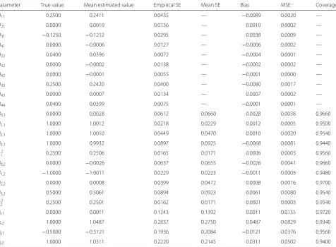
and results from 500 simulations are shown in Table3. In particular, we display the mean estimate, the bias, the empirical SE (= the standard deviation of the the
parameter estimates); the mean SE (= the mean SE
of each parameter calculated for each fitted model); the mean square error (MSE), and the coverage. The results confirm that the model fitting algorithm generally performs well.
A second simulation analysis was conducted using the parameters above (withn = 100 subjects per dataset).
However, in this case we used a heavier-tailed distribu-tion for the random effects: a multivariate t5 distribu-tion [40]. The bias for the fixed effect coefficients was comparable to the multivariate normal random effects simulation study (above). The empirical standard error was consistently smaller than the mean standard error, resulting in coverage between 95% and 99% for the coef-ficient parameters. Rizopoulos et al. [41] noted that the misspecification of the random effects distributions was minimised as the number of longitudinal measurements per subject increased, but that the standard errors are gen-erally affected. These findings are broadly in agreement with the simulation study conducted here, and other stud-ies [42,43]. Choi et al. [44] provide a review of existing research on the misspecification of random effects in joint modelling.
Example
Table 3Results of simulation study
Parameter True value Mean estimated value Empirical SE Mean SE Bias MSE Coverage
D11 0.2500 0.2411 0.0435 — −0.0089 0.0020 —
D21 0.0000 0.0010 0.0136 — 0.0010 0.0002 —
D31 −0.1250 −0.1212 0.0295 — 0.0038 0.0009 —
D41 0.0000 −0.0006 0.0127 — −0.0006 0.0002 —
D22 0.0400 0.0396 0.0072 — −0.0004 0.0001 —
D32 0.0000 −0.0002 0.0138 — −0.0002 0.0002 —
D42 0.0000 −0.0001 0.0055 — −0.0001 0.0000 —
D33 0.2500 0.2420 0.0400 — −0.0080 0.0017 —
D43 0.0000 0.0007 0.0134 — 0.0007 0.0002 —
D44 0.0400 0.0399 0.0075 — −0.0001 0.0001 —
β0,1 0.0000 0.0028 0.0612 0.0660 0.0028 0.0038 0.9660
β1,1 1.0000 1.0012 0.0218 0.0229 0.0012 0.0005 0.9500
β2,1 1.0000 1.0010 0.0449 0.0470 0.0010 0.0020 0.9540
β3,1 1.0000 0.9932 0.0897 0.0925 −0.0068 0.0081 0.9440
σ2
1 0.2500 0.2506 0.0165 0.0171 0.0006 0.0003 0.9560
β0,2 0.0000 −0.0026 0.0637 0.0655 −0.0026 0.0041 0.9660
β1,2 −1.0000 −1.0011 0.0229 0.0223 −0.0011 0.0005 0.9480
β2,2 0.0000 0.0008 0.0399 0.0472 0.0008 0.0016 0.9700
β3,2 0.5000 0.5061 0.0894 0.0923 0.0061 0.0080 0.9540
σ2
2 0.2500 0.2501 0.0162 0.0171 0.0001 0.0003 0.9540
γv1 0.0000 0.0011 0.1243 0.1392 0.0011 0.0155 0.9720
γv2 1.0000 1.0487 0.2837 0.2750 0.0487 0.0829 0.9340
γy1 −0.5000 −0.5121 0.1936 0.2084 −0.0121 0.0376 0.9560
γy2 1.0000 1.0311 0.2220 0.2145 0.0311 0.0502 0.9400
Patients with PBC typically have abnormalities in sev-eral blood tests; hence, during follow-up sevsev-eral biomark-ers associated with liver function were serially recorded for these patients. We consider three biomarkers: serum
bilirunbin (denoted serBilir in the model and data;
measured in units of mg/dl), serum albumin (albumin; mg/dl), and prothrombin time (prothrombin; seconds).
Patients had a mean 6.3 (SD = 3.7) visits (including
baseline). The data can be accessed from thejoineRML
package via the command data(pbc2). Profile plots
for each biomarker are shown in Fig. 1, indicating
distinct differences in trajectories between the those who died during follow-up and those who did not (right-censored cases). A Kaplan-Meier curve for
over-all survival is shown in Fig. 2. There were a total
of 69 (44.8%) deaths during follow-up in the placebo subset.
We fit a relatively simple joint model for the purposes of demonstration, which encompasses the following trivari-ate longitudinal data sub-model:
log(serBilir)=(β0,1+b0i,1)+(β1,1+b1i,1)year+εij1,
albumin=(β0,2+b0i,2)+(β1,2+b1i,2)year+εij2, (0.1×prothrombin)−4=(β0,3+b0i,3)+(β1,3+b1i,3)year+εij3,
bi∼N6(0,D), andεijk∼N(0,σk2)fork=1,2,3; and a time-to-event sub-model for the study endpoint of death:
λi(t) = λ0(t)exp{γvagei+W2i(t)},
W2i(t) = γbil(b0i,1+b1i,1t)+γalb(b0i,2+b1i,2t)
+ γpro(b0i,3+b1i,3t).
The log transformation of bilirubin is standard, and confirmed reasonable based on inspection of Q-Q plots for residuals from a separate fitted linear mixed model
fitted using the lme() function from the R package
Fig. 1Longitudinal trajectory plots. The black lines show individual subject trajectories, and the coloured lines show smoothed (LOESS) curves stratified by whether the patient experienced the endpoint (blue) or not (red)
which was confirmed by inspection of a Q-Q plot. The pairwise correlations for baseline measurements between the three transformed markers were 0.19 (pro-thrombin time vs. albumin), −0.30 (bilirubin vs. pro-thrombin time and albumin). The model is fit using the joineRML R package (version 0.2.0) using the following code.
Fig. 2Kaplan-Meier curve for overall survival. A pointwise 95% band is shown (dashed lines). In total, 69 patients (of 154) died during follow-up
# Get data data(pbc2)
placebo <- subset(pbc2, drug == "placebo") # Fit model
fit.pbc <- mjoint( formLongFixed = list(
"bil" = log(serBilir) ~ year, "alb" = albumin ~ year,
"pro" = (0.1 * prothrombin)^-4 ~ year), formLongRandom = list(
"bil" = ~ year | id, "alb" = ~ year | id, "pro" = ~ year | id),
formSurv = Surv(years, status2) ~ age, data = placebo,
timeVar = "year",
control = list(tol0 = 0.001, burnin = 400) )
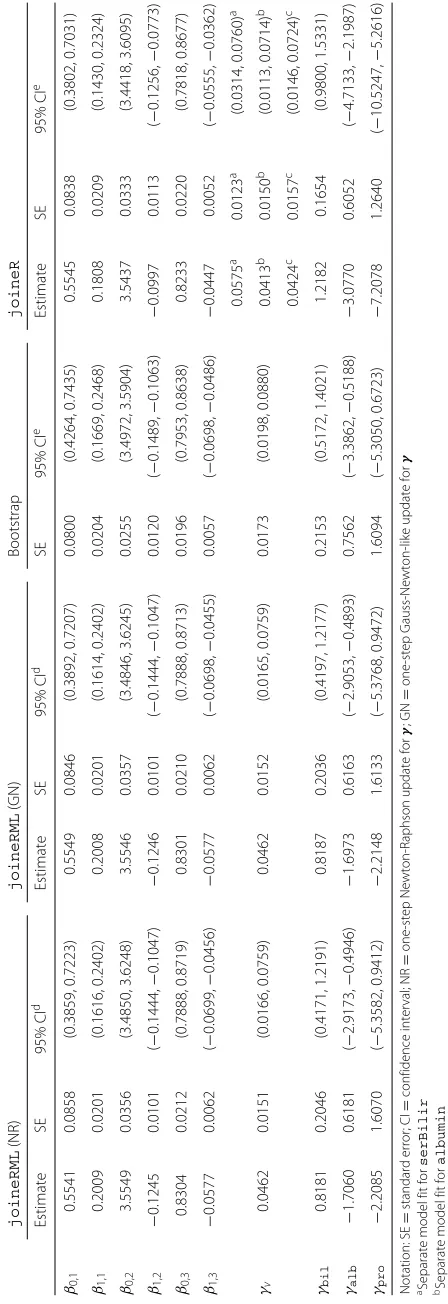
Table 4 Fitted multivariate and separate univariate joint models to the PBC data joineRML (NR) joineRML (GN) Bootstrap joineR Estimate SE 95% CI d Estimate SE 95% CI d SE 95% CI e Estimate SE 95% CI e β0,1 0.5541 0.0858 (0.3859, 0.7223) 0.5549 0.0846 (0.3892, 0.7207) 0.0800 (0.4264, 0.7435) 0.5545 0.0838 (0.3802, 0.7031) β1,1 0.2009 0.0201 (0.1616, 0.2402) 0.2008 0.0201 (0.1614, 0.2402) 0.0204 (0.1669, 0.2468) 0.1808 0.0209 (0.1430, 0.2324) β0,2 3.5549 0.0356 (3.4850, 3.6248) 3.5546 0.0357 (3.4846, 3.6245) 0.0255 (3.4972, 3.5904) 3.5437 0.0333 (3.4418, 3.6095) β1,2 − 0.1245 0.0101 ( − 0.1444, − 0.1047) − 0.1246 0.0101 ( − 0.1444, − 0.1047) 0.0120 ( − 0.1489, − 0.1063) − 0.0997 0.0113 ( − 0.1256, − 0.0773) β0,3 0.8304 0.0212 (0.7888, 0.8719) 0.8301 0.0210 (0.7888, 0.8713) 0.0196 (0.7953, 0.8638) 0.8233 0.0220 (0.7818, 0.8677) β1,3 − 0.0577 0.0062 ( − 0.0699, − 0.0456) − 0.0577 0.0062 ( − 0.0698, − 0.0455) 0.0057 ( − 0.0698, − 0.0486) − 0.0447 0.0052 ( − 0.0555, − 0.0362) γv 0.0462 0.0151 (0.0166, 0.0759) 0.0462 0.0152 (0.0165, 0.0759) 0.0173 (0.0198, 0.0880) 0.0575 a 0.0123 a (0.0314, 0.0760) a 0.0413 b 0.0150 b (0.0113, 0.0714) b 0.0424 c 0.0157 c (0.0146, 0.0724) c γbil 0.8181 0.2046 (0.4171, 1.2191) 0.8187 0.2036 (0.4197, 1.2177) 0.2153 (0.5172, 1.4021) 1.2182 0.1654 (0.9800, 1.5331) γalb − 1.7060 0.6181 ( − 2.9173, − 0.4946) − 1.6973 0.6163 ( − 2.9053, − 0.4893) 0.7562 ( − 3.3862, − 0.5188) − 3.0770 0.6052 ( − 4.7133, − 2.1987) γpro − 2.2085 1.6070 ( − 5.3582, 0.9412) − 2.2148 1.6133 ( − 5.3768, 0.9472) 1.6094 ( − 5.3050, 0.6723) − 7.2078 1.2640 ( − 10.5247, − 5.2616) Notation: SE = standard error; CI = confidence interval; N R = one-step Newton-Raphson update for γ ;G N = one-step Gauss-Newton-like update for γ aSeparate model fit for serBilir bSeparate model fit for albumin cSeparate model fit for prothrombin dSEs are calculated from the inverse p rofile empirical information matrix, and confidence intervals are based o n n ormal approximations of the type
ˆθ±
1.96SE
(
ˆθ),w
h
e
re
ˆθdenote
The fitted model indicated that an increase in the subject-specific random deviation from the population trajectory of serum bilirubin was significantly associated with increased hazard of death. A significant association was also detected for subject-specific decreases in albu-min from the population mean trajectory. However, prothrombin time was not significantly associated with hazard of death, although its direction is clinically con-sistent with PBC disease. Albert and Shih [46] analysed the first 4-years follow-up from this dataset with the same 3 biomarkers and a discrete event time distribution using a regression calibration model. Their results were broadly consistent, although the effect of prothrombin time on the event time sub-model was strongly significant.
We also fitted 3 univariate joint models to each of the biomarkers and the event time sub-model using the R package joineR (version 1.2.0) owing to its optimiza-tion for such models. The LMM parameter estimates were similar, although the absolute magnitude of the slopes was smaller for the separate univariate models. Since 3 separate models were fitted, 3 estimates ofγv were esti-mated, with the average comparable to the multivariate model estimate. The multivariate model estimates ofγy=
(γbil,γalb,γpro)were substantially attenuated relative to the separate model estimates, although the directions remained consistent. It is also interesting to note that
γpro was statistically significant in the univariate model. However, the univariate models are not accounting for the correlation between different outcomes, whereas the multivariate joint model does.
The model was refitted with the one-step
Newton-Raphson update forγ replaced by a Gauss-Newton-like
update in a time of 2.2 minutes for 419 MCEM iterations with a final MC size ofM=6272. This is easily achieved by running the following code.
fit.pbc.gn <- update(fit.pbc,gammaOpt = "GN")
In addition, we bootstrapped this model withB = 100
samples to estimate SEs and contrast them with the approximate estimates based on the inverse empirical pro-file information matrix. In practice, one should choose B > 100, particularly if using bootstrap percentile confi-dence intervals; however, we used a small value to reduce the computational burden on this process. In a similar spirit, we relaxed the convergence criteria and reduced the number of burn-in iterations. This is easily implemented by running the following code, taking 1.8 h to fit.
fit.pbc.gn.boot <- bootSE(fit.pbc.gn, nboot = 100, control = list(
tol0 = 0.005, tol2 = 0.01, convCrit = "sas",
burnin = 300, mcmaxIter = 350))
It was observed that the choice of gradient matrix in the
γ-update led to virtually indistinguishable parameter esti-mates, although we note the same random seed was used in both cases. The bootstrap estimated SEs were broadly consistent with the approximate SEs, with no consistent pattern in underestimation observed.
Discussion
Multivariate joint models introduce three types of corre-lations: (1) within-subject serial correlation for repeated measures; (2) between longitudinal outcomes correla-tion; and (3) correlation between the multivariate LMM and time-to-event sub-models. It is important to account for all of these types of correlations; however, some authors have reported collapsing their multivariate data to permit univariate joint models to be fitted. For
example, Battes et al. [7] used an ad hoc approach
of either summing or multiplying the three repeated continuous measures (standardized according to clini-cal upper reference limits of the biomarker assays), and then applying standard univariate joint models. Wang et al. [48] fitted separate univariate joint models to each longitudinal outcome in turn. Neither approach takes complete advantage of the correlation between the multiple longitudinal measures and the time-to-event outcome.
Here, we described a new R package joineRML that
can fit the models described in this paper. This was demonstrated on a real-world dataset. Although in the fit-ted model we assumed linear trajectories for the biomark-ers, splines could be straightforwardly employed, as have been used in other multivariate joint model applications [15], albeit at the cost of additional computational time. Despite a growing availability of software for univariate joint models, Hickey et al. [19] noted that there were very few options for fitting joint models involving multi-variate longitudinal data. To the best of our knowledge, options are limited to the R packages JMbayes [49], rstanarm[50], and the Stata packagestjm[47]. More-over, none of these incorporates an unspecified baseline hazard. The first two packages use Markov chain Monte Carlo (MCMC) methods to fit the joint models. Bayesian models are potentially very useful for fitting joint mod-els, and in particular for dynamic prediction; however, MCMC is also computationally demanding, especially in the case of multivariate models. Several other publications
have madeBUGS code available for use with WinBUGS
and OpenBUGS (e.g. [51]), but these are not easily modi-fiable and post-fit computations are cumbersome.
joineRML is a new software package developed to fill a void in the joint modelling field, but is still in its infancy relative to highly developed univariate joint model packages such as the R packageJM[28] and Stata
intend to cover several deficiencies. First, joineRML currently only permits an association structure of the form W2i(t) = #Kk=1γykW1(k)i (t). As has been demon-strated by others, the association might take different forms, including random-slopes and cumulative effects or some combination of multiple structures, and these may also be different for separate longitudinal outcomes [18]. Moreover, it is conceivable that separate longitu-dinal outcomes may interact in the hazard sub-model. Second, the use of MC integration provides a scalable solution to the issue of increasing dimensionality in the random effects. However, for simpler cases, e.g. bivari-ate models with random-intercepts and random-slopes (total of 4 random effects), Gaussian quadrature might be computationally superior; this trade-off requires fur-ther investigation. Third,joineRML can currently only model a single event time. However, there is a grow-ing interest in competgrow-ing risks [9] and recurrent events data [11], which if incorporated intojoineRML, would provide a flexible all-round multivariate joint modelling platform. Competing risks [28,29] and recurrent events [38] have been incorporated into joint modelling R pack-ages already, but are limited to the case of a solitary longitudinal outcome. Of note, the PBC trial dataset anal-ysed in this study includes times to the competing risk of liver transplantation. Fourth, with ever-increasing vol-umes of data collected during routine clinical visits, the need for software to fit joint models with very many lon-gitudinal outcomes is foreseeable [52]. This would likely require the use of approximate methods for the numerical integration or data reduction methods. Fifth, additional residual diagnostics are necessary for assessing possible violations of model assumptions. ThejoineRMLpackage has aresid()function for extracting the longitudinal sub-model residuals; however, these are complex for diag-nostic purposes due to the informative dropout, hence the development of multiple-imputation based residuals [53].
Conclusions
In this paper we have presented an extension of the clas-sical joint model proposed by Henderson et al. [3] and an estimation procedure for fitting the models that builds on the foundations laid by Lin et al. [20]. In addition,
we described a new R package joineRML that can fit
the models described in this paper, which leverages the MCEM algorithm and which should scale well for increas-ing number of longitudinal outcomes. This software is timely, as it has previously been highlighted that there is a paucity of software available to fit such models [19]. The software is being regularly updated and improved.
Availability and requirements Project name:joineRML
Project home page:https://github.com/graemeleehickey/
joineRML/
Operating system(s):platform independent Programming language:R
Other requirements:none License:GNU GPL-3
Any restrictions to use by non-academics: none
Additional file
Additional file 1: An appendix (appendix.pdf) is available that includes details on the score vector and M-step estimators. (PDF 220 kb)
Abbreviations
BLUP: Best linear unbiased prediction; CRAN: The Comprehensive R Archive Network; EM: Expectation maximisation; LMM: Linear mixed models; MC: Monte Carlo; MCEM: Monte Carlo expectation maximisation; MLE: Maximum likelihood estimate; PBC: Primary biliary cirrhosis; SD: Standard deviation; SE: Standard error
Acknowledgements
The authors would like to thank Professor Robin Henderson (University of Newcastle) for useful discussions with regards to the MCEM algorithm, and Dr Haiqun Lin (Yale University) for helpful discussions on the likelihood specification.
Funding
Funding for the project was provided by the Medical Research Council (Grant number MR/M013227/1). The funder had no role in the design of the study and collection, analysis, and interpretation of data and in writing the manuscript.
Availability of data and materials
The R packagejoineRMLcan be installed directly usinginstall.package s("joineRML")in an R console. The source code is available athttps:// github.com/graemeleehickey/joineRML. Archived versions are available from the Comprehensive R Archive Network (CRAN) athttps://cran.r-project.org/ web/packages/joineRML/.joineRMLis platform independent, requiring R version≥3.3.0, and is published under a GNU GPL-3 license. The dataset analysed during the current study is bundled with the R packagejoineRML, and can be accessed by running the commanddata(pbc2, package = "joineRML").
Authors’ contributions
All authors collaborated in developing the model fitting algorithm reported. The programming and running of the analysis was carried out by GLH. GLH wrote the first draft of the manuscript, with input provided by PP, AJ, and RKD. All authors contributed to the manuscript revisions. All authors read and approved the final manuscript.
Ethics approval and consent to participate Not applicable.
Competing interests
The authors declare that they have no competing interests.
Publisher’s Note
Springer Nature remains neutral with regard to jurisdictional claims in published maps and institutional affiliations.
Author details
1Department of Biostatistics, Institute of Translational Medicine, University of Liverpool, Waterhouse Building, 1-5 Brownlow Street, L69 3GL Liverpool, UK. 2Department of Mathematics, Physics and Electrical Engineering, Northumbria University, Ellison Place, NE1 8ST Newcastle upon Tyne, UK.
References
1. Ibrahim JG, Chu H, Chen LM. Basic concepts and methods for joint models of longitudinal and survival data. J Clin Oncol. 2010;28(16): 2796–801.
2. Sweeting MJ, Thompson SG. Joint modelling of longitudinal and time-to-event data with application to predicting abdominal aortic aneurysm growth and rupture. Biom J. 2011;53(5):750–63. 3. Henderson R, Diggle PJ, Dobson A. Joint modelling of longitudinal
measurements and event time data. Biostatistics. 2000;1(4):465–480. 4. Tsiatis AA, Davidian M. Joint modeling of longitudinal and time-to-event
data: an overview. Stat Sin. 2004;14:809–34.
5. Gould AL, Boye ME, Crowther MJ, Ibrahim JG, Quartey G, Micallef S, Bois FY. Joint modeling of survival and longitudinal non-survival data: current methods and issues. report of the DIA Bayesian joint modeling working group. Stat Med. 2015;34:2181–95.
6. Rizopoulos D. Joint Models for Longitudinal and Time-to-Event Data, with Applications in R. Boca Raton: Chapman & Hall/CRC; 2012.
7. Battes LC, Caliskan K, Rizopoulos D, Constantinescu AA, Robertus JL, Akkerhuis M, Manintveld OC, Boersma E, Kardys I. Repeated measurements of NT-pro-B-type natriuretic peptide, troponin T or C-reactive protein do not predict future allograft rejection in heart transplant recipients. Transplantation. 2015;99(3):580–5.
8. Song X, Davidian M, Tsiatis AA. An estimator for the proportional hazards model with multiple longitudinal covariates measured with error. Biostatistics. 2002;3(4):511–28.
9. Williamson P, Kolamunnage-Dona R, Philipson P, Marson AG. Joint modelling of longitudinal and competing risks data. Stat Med. 2008;27: 6426–38.
10. Hickey GL, Philipson P, Jorgensen A, Kolamunnage-Dona R.
A comparison of joint models for longitudinal and competing risks data, with application to an epilepsy drug randomized controlled trial. J R Stat Soc: Ser A: Stat Soc. 2018.https://doi.org/10.1111/rssa.12348.
11. Liu L, Huang X. Joint analysis of correlated repeated measures and recurrent events processes in the presence of death, with application to a study on acquired immune deficiency syndrome. J R Stat Soc: Ser C: Appl Stat. 2009;58(1):65–81.
12. Chi YY, Ibrahim JG. Joint models for multivariate longitudinal and multivariate survival data. Biometrics. 2006;62(2):432–45. 13. Hickey GL, Philipson P, Jorgensen A, Kolamunnage-Dona R. Joint
models of longitudinal and time-to-event data with more than one event time outcome: a review. Int J Biostat. 2018. https://doi.org/10.1515/ijb-2017-0047.
14. Andrinopoulou E-R, Rizopoulos D, Takkenberg JJM, Lesaffre E. Combined dynamic predictions using joint models of two longitudinal outcomes and competing risk data. Stat Methods Med Res. 2017;26(4):1787–1801. 15. Rizopoulos D, Ghosh P. A Bayesian semiparametric multivariate joint
model for multiple longitudinal outcomes and a time-to-event. Stat Med. 2011;30(12):1366–80.
16. Faucett CL, Thomas DC. Simultaneously modelling censored survival data and repeatedly measured covariates: a Gibbs sampling approach. Stat Med. 1996;15(15):1663–85.
17. Song X, Davidian M, Tsiatis AA. A semiparametric likelihood approach to joint modeling of longitudinal and time-to-event data. Biometrics. 2002;58(4):742–53.
18. Andrinopoulou E-R, Rizopoulos D. Bayesian shrinkage approach for a joint model of longitudinal and survival outcomes assuming different association structures. Stat Med. 2016;35(26):4813–23.
19. Hickey GL, Philipson P, Jorgensen A, Kolamunnage-Dona R. Joint modelling of time-to-event and multivariate longitudinal outcomes: recent developments and issues. BMC Med Res Methodol. 2016;16(1): 1–15.
20. Lin H, McCulloch CE, Mayne ST. Maximum likelihood estimation in the joint analysis of time-to-event and multiple longitudinal variables. Stat Med. 2002;21:2369–82.
21. Laird NM, Ware JH. Random-effects models for longitudinal data. Biometrics. 1982;38(4):963–74.
22. Wei GC, Tanner MA. A Monte Carlo implementation of the EM algorithm and the poor man’s data augmentation algorithms. J Am Stat Assoc. 1990;85(411):699–704.
23. Wulfsohn MS, Tsiatis AA. A joint model for survival and longitudinal data measured with error. Biometrics. 1997;53(1):330–9.
24. Ratcliffe SJ, Guo W, Ten Have TR. Joint modeling of longitudinal and survival data via a common frailty. Biometrics. 2004;60(4):892–9. 25. McLachlan GJ, Krishnan T. The EM Algorithm and Extensions, 2nd ed.
Hoboken: Wiley-Interscience; 2008.
26. Pinheiro JC, Bates DM. Mixed-Effects Models in S and S-PLUS. New York: Springer; 2000.
27. Therneau TM, Grambsch PM. Modeling Survival Data: Extending the Cox Model. New Jersey: Springer; 2000, p. 350.
28. Rizopoulos D. JM: an R package for the joint modelling of longitudinal and time-to-event data. Journal of Statistical Software. 2010;35(9):1–33. 29. Philipson P, Sousa I, Diggle PJ, Williamson P, Kolamunnage-Dona R,
Henderson R, Hickey GL. joineR: Joint Modelling of Repeated Measurements and Time-to-event Data. 2017. R package version 1.2.0. https://CRAN.R-project.org/package=joineR.
30. Dmitrienko A, Molenberghs G, Chuang-Stein C, Offen W. Analysis of Clinical Trials Using SAS: A Practical Guide. Cary: SAS Institute; 2005. 31. Law NJ, Taylor JM, Sandler H. The joint modeling of a longitudinal
disease progression marker and the failure time process in the presence of cure. Biostatistics. 2002;3(4):547–63.
32. McCulloch CE. Maximum likelihood algorithms for generalized linear mixed models. J Am Stat Assoc. 1997;92(437):162–70.
33. Booth JG, Hobert JP. Maximizing generalized linear mixed model likelihoods with an automated Monte Carlo EM algorithm. J R Stat Soc Ser B Stat Methodol. 1999;61(1):265–85.
34. Ripatti S, Larsen K, Palmgren J. Maximum likelihood inference for multivariate frailty models using an automated Monte Carlo EM algorithm. Lifetime Data Anal. 2002;8(2002):349–60.
35. Hsieh F, Tseng YK, Wang JL. Joint modeling of survival and longitudinal data: Likelihood approach revisited. Biometrics. 2006;62(4):1037–43. 36. Xu C, Baines PD, Wang JL. Standard error estimation using the EM
algorithm for the joint modeling of survival and longitudinal data. Biostatistics. 2014;15(4):731–44.
37. Eddelbuettel D, Sanderson C. RcppArmadillo: accelerating r with high-performance C++ linear algebra. Comput Stat Data Anal. 2014;71: 1054–63.
38. Król A, Mauguen A, Mazroui Y, Laurent A, Michiels S, Rondeau V. Tutorial in joint modeling and prediction: A statistical software for correlated longitudinal outcomes, recurrent events and a terminal event. J Stat Softw. 2017;81(3):1–52.
39. Austin PC. Generating survival times to simulate Cox proportional hazards models with time-varying covariates. Stat Med. 2012;31(29):3946–58. 40. Genz A, Bretz F. Computation of Multivariate Normal and t Probabilities.
Berlin: Springer; 2009.
41. Rizopoulos D, Verbeke G, Molenberghs G. Shared parameter models under random-effects misspecification. Biometrika. 2008;95(1):63–74. 42. Xu J, Zeger SL. The evaluation of multiple surrogate endpoints.
Biometrics. 2001;57(1):81–7.
43. Pantazis N, Touloumi G. Robustness of a parametric model for informatively censored bivariate longitudinal data under misspecification of its distributional assumptions: a simulation study. Stat Med. 2007;26: 5473–85.
44. Choi J, Zeng D, Olshan AF, Cai J. Joint modeling of survival time and longitudinal outcomes with flexible random effects. Lifetime Data Anal. 2018;24(1):126–52.
45. Murtaugh PA, Dickson ER, Van Dam GM, Malinchoc M, Grambsch PM, Langworthy AL, Gips CH. Primary biliary cirrhosis: prediction of short-term survival based on repeated patient visits. Hepatology. 1994;20(1):126–134. 46. Albert PS, Shih JH. An approach for jointly modeling multivariate
longitudinal measurements and discrete time-to-event data. Ann Appl Stat. 2010;4(3):1517–32.
47. Crowther MJ, Abrams KR, Lambert PC. Joint modeling of longitudinal and survival data. Stata J. 2013;13(1):165–84.
48. Wang P, Shen W, Boye ME. Joint modeling of longitudinal outcomes and survival using latent growth modeling approach in a mesothelioma trial. Health Serv Outcome Res Methodol. 2012;12(2–3):182–99.
49. Rizopoulos D. The R package JMbayes for fitting joint models for longitudinal and time-to-event data using mcmc. J Stat Softw. 2016;72(7): 1–45.
51. Andrinopoulou E-R, Rizopoulos D, Takkenberg JJM, Lesaffre E. Joint modeling of two longitudinal outcomes and competing risk data. Stat Med. 2014;33(18):3167–78.
52. Jaffa MA, Gebregziabher M, Jaffa AA. A joint modeling approach for right censored high dimensiondal multivariate longitudinal data. J Biom Biostat. 2014;5(4):1000203.