Estimates of vertical eddy diffusivity in the upper mesosphere in the
presence of a mesospheric inversion layer
R. L. Collins1, G. A. Lehmacher2, M. F. Larsen2, and K. Mizutani3
1Geophysical Institute and Department of Atmospheric Sciences, University of Alaska Fairbanks, 903 Koyukuk Drive, Fairbanks, AK 99775-7320, USA
2Department of Physics and Astronomy, Clemson University, 118 Kinard Laboratory, Clemson, SC 29631-0978, USA 3Environmental Sensing and Network Group, National Institute of Information and Communications Technology, 4-2-1 Nukui-kita, Koganei, Tokyo 184-8795, Japan
Received: 21 May 2011 – Revised: 13 August 2011 – Accepted: 27 September 2011 – Published: 15 November 2011
Abstract. Rayleigh and resonance lidar observations were made during the Turbopause experiment at Poker Flat Re-search Range, Chatanika Alaska (65◦N, 147◦W) over a 10 h period on the night of 17–18 February 2009. The lidar ob-servations revealed the presence of a strong mesospheric in-version layer (MIL) at 74 km that formed during the obser-vations and was present for over 6 h. The MIL had a maxi-mum temperature of 251 K, amplitude of 27±7 K, a depth of 3.0 km, and overlying lapse rate of 9.4±0.3 K km−1. The MIL was located at the lower edge of the mesospheric sodium layer. During this coincidence the lower edge of the sodium layer was lowered by 2 km to 74 km and the bot-tomside scale height of the sodium increased from 1 km to 15 km. The structure of the MIL and sodium are analyzed in terms of vertical diffusive transport. The analysis yields a lower bound for the eddy diffusion coefficient of 430 m2s−1 and the energy dissipation rate of 2.2 mW kg−1at 76–77 km. This value of the eddy diffusion coefficient, determined from naturally occurring variations in mesospheric temperatures and the sodium layer, is significantly larger than those re-ported for mean winter values in the Arctic but similar to in-dividual values reported in regions of convective instability by other techniques.
Keywords. Meteorology and atmospheric dynamics (Mid-dle atmosphere dynamics; Turbulence; Instruments and tech-niques)
Correspondence to: R. L. Collins ([email protected])
1 Introduction
Turbulence is critical in determining the vertical distribution and transport of minor species in the middle atmosphere as well as contributing to the dissipation of waves and tides in this region. The dynamical processes of gravity-wave in-stability, overturning, breaking, and nonlinear behavior both contribute to turbulent processes in the mesosphere and are impacted by them (see the collection of papers in the mono-graph edited by Siskind et al., 2000; and the review arti-cles by Fritts and Alexander, 2003; Hecht, 2004). Efforts to characterize turbulence vary between attempts to describe the time-averaged behavior that supports studies of the com-position and circulation of the middle atmosphere at sea-sonal and climatological time-scales (e.g., Schoeberl et al., 1983; Vlasov and Kelley, 2010) and attempts to describe the small-scale transient processes that generate turbulence lo-cally (e.g., Lehmacher and L¨ubken, 1995; Hecht et al., 1997; Bishop et al., 2004; Lehmacher et al., 2006). Furthermore there are significant differences in the techniques used to measure turbulence that tend to yield systematic differences in the values of turbulent parameters (e.g., L¨ubken, 1997; Hecht et al., 2004).
the Turbopause experiment. The lidar observations were Rayleigh lidar measurements of temperature profile (∼40– 90 km) and resonance lidar measurements of mesospheric sodium profiles (∼70–120 km). The rocket-based measure-ments coincided with the appearance of a mesospheric inver-sion layer near 75 km, with an overlying near adiabatic lapse rate, and changes in the structure of the bottomside of the sodium layer at the same altitude. We analyze these observa-tions in terms of recent studies of wave-breaking, turbulence, and sodium chemistry and estimate the eddy diffusivity asso-ciated with the mesospheric inversion layer.
This paper is arranged as follows. In Sect. 2 we describe the Rayleigh and resonance lidar techniques and the methods used to determine and characterize the thermal structure and the sodium layer. In Sect. 3 we present the lidar observations in terms of the mesospheric inversion layer and the coinci-dent structure of the sodium layer. In Sect. 4 we analyze the observations in terms of turbulent transport and estimate the eddy diffusion coefficient. In Sect. 5 we discuss our obser-vations and results in terms of other studies of turbulence. Finally, in Sect. 6 we present our summary and conclusions.
2 Experiment and methods
2.1 Rayleigh lidar
Rayleigh lidar measurements of middle atmosphere tempera-tures have been made at Chatanika on an ongoing basis since 1997 (Thurairajah et al., 2009). The configuration of the li-dar system during the Turbopause experiment was the same as that reported in recent studies (e.g., Thurairajah et al., 2010a, b). The lidar observations yielded measurements of the stratospheric and mesospheric temperature profile (∼40– 80 km) under the assumptions of hydrostatic equilibrium and an initial temperature at the upper altitude. In previous stud-ies we had taken the initial temperature values from a climate atlas. The initial temperature was the major source of uncer-tainty in the lidar measurement in the altitude range within a scale height (∼8 km) of the upper altitude. In this study we used the Turbopause rocket-borne ionization gauge measure-ments of temperature (Lehmacher et al., 2011) to provide the temperature at the upper altitude and thus remove this source of uncertainty from the lidar measurements. The Turbopause rocket-borne measurements were made with four rockets launched over a period of two hours. The ionization gauge measurements were made during the downleg stage of two of the rockets that were launched at 01:29 LST (10:29 UT) and 01:59 LST (10:59 UT). The resolution of the Rayleigh lidar measurements was 50 s and 75 m. We then integrate the Rayleigh lidar data to improve the statistical confidence in the temperature measurements. Except for the choice of ini-tial temperature, we use the same inversion methods as those reported in recent studies (e.g., Thurairajah et al., 2010b). We operated the Rayleigh lidar over an 11 h period from
19:47 until 07:12 on the night of 17–18 February 2009 LST (04:47–16:12, 18 February 2009 UT, UT = LST + 9 h).
In this study we report temperature profiles for both the entire night over the 40–90 km altitude range and successive 2-h intervals over the 40–82 km altitude range. When we consider the temperature structure at the time of the rocket-borne measurements (i.e., profiles based on the integration over the 2-h intervals centered on the rocket-borne measure-ment), we use the corresponding ionization gauge tempera-ture measurement as the initial temperatempera-ture in the lidar in-version. When we consider the temperature structure for the whole night (i.e., the nightly mean or a sequence of 2-h pro-files), we use the average of the ionization gauge temperature measurements as the initial temperature in the lidar inversion. We determine the uncertainty in the measurements due to the initial temperature by calculating the variation in the mea-sured temperatures due to changes in the initial temperature (±10 K,±25 K).
2.2 Resonance lidar
Resonance lidar measurements of the mesospheric sodium layer have been made at Chatanika on an ongoing basis since 1995 (Collins et al., 1996; Collins and Smith, 2004). The configuration of the resonance lidar during the Turbopause experiment differed from that reported by Collins and Smith (2004). For this experiment we replaced the 0.35 m diameter telescope with a 1.04 m diameter telescope, and we replaced the flashlamp-pumped dye laser with an excimer-pumped dye laser. Consequently due to the increase in the receiver area, increase in the laser power, reduction in laser linewidth, and increase in laser frequency stability, the lidar signal lev-els were a factor 10–20 times greater than in earlier studies at Chatanika. The resolution of the resonance lidar measure-ments was 100 s and 75 m. We then integrated the resonance lidar data to 15 min to improve the statistical confidence in the sodium measurements. We used the same standard in-version methods as used in previous studies to determine the sodium concentration profiles between 70 and 120 km. We operated the resonance lidar over a 10 h period from 20:35 until 06:00 LST (05:35–15:00 UT).
3 Observations
3.1 Stratospheric and mesospheric temperature
Fig. 1. Temperature profiles measured by Rayleigh lidar at Chatanika, Alaska on the night of 17–18 February 2009. The nightly average temperature measured over the interval 19:47– 07:12 LST (04:47–16:12 UT, thick dashed line) and the tempera-ture profile measured over the two hour interval 01:04–03:04 LST (10:04–12:04 UT, thin solid line) are plotted. The one-sigma tem-perature errors due to the statistical fluctuations in the lidar signal (dashed lines) and the SPARC February temperature profile (dashed line and solid squares) are also plotted. The linear fit to the topside of the mesospheric inversion layer is indicated.
altitude of 49.8 km and had a temperature of 235.1 K. The SPARC stratopause was at 49.1 km and had a temperature of 253.4 K, nearly 20 K warmer than the lidar measurement. The lidar measurement also shows a mesospheric inversion layer (MIL) that extended from 67.6 km to 73.2 km. The MIL had a maximum temperature of 232.5 K, amplitude of 9.8±2.3 K, and a depth of 5.6 km. We determined the lapse rate over 3 km intervals on the topside of the MIL and find that the maximum lapse rate was 4.7±0.2 K km−1over the 76.8–79.8 km range.
We calculated the temperature profiles over the two-hour period spanning the rocket-borne ionization gauge measure-ment at 02:04 LST (11:04 UT). We initialized the tempera-ture profile with the ionization gauge measurement at 82 km. The temperature profile is plotted in Fig. 1. The MIL is clearly evident. The 01:04–03:04 LST profile shows a MIL that extends from 71.2 km to 74.2 km. The MIL has a maxi-mum temperature of 251.0 K, amplitude of 27.2±6.8 K, and a depth of 3.0 km. We find that the maximum lapse rate is 9.4±0.3 K km−1over the 74.5–77.5 km range. MILs of similar amplitude have been reported at Chatanika at lower altitudes (Cutler et al., 2001). In order to study the evolu-tion of the MIL over the entire observaevolu-tion period we calcu-lated a sequence of 19 temperature profiles that are derived from the Rayleigh lidar signal integrated over 2 h intervals at 30 min offset. Given the proximity of the MIL to the ini-tial ionization gauge temperature, we also calculated the
se-Fig. 2. Characteristics of mesospheric inversion layer (MIL)
mea-sured by Rayleigh lidar at Chatanika Alaska on the morning of 18 February 2009 (solid thick line closed square). The values due to errors in the initial temperature at 82 km (long dashed lines) are also plotted. Upper: Peak MIL altitude as function of local time. Middle: MIL Amplitude, as a function of time. The error bars are one-sigma uncertainties due to the statistical fluctuation in the lidar signal. Lower: MIL Lapse Rate as a function of time. The error bars are one-sigma uncertainties due to the statistical fluctuation in the li-dar signal. The dry adiabatic lapse rate is also plotted (short dashed line). The maximum, minimum and average values are noted.
quence of temperature profiles using the initial temperature
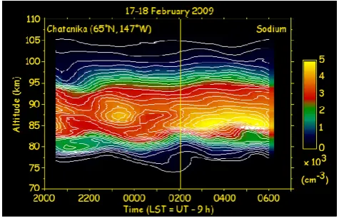
[image:3.595.49.282.63.243.2]Fig. 3. Sodium concentration measured by resonance lidar at Chatanika, Alaska on the night of 17–18 February 2009. The concentration is plotted in false color as a function of time (LST = UT−9 h) and altitude. The concentrations have been low pass filtered with Parzen filters having cut-offs of 1 km and 2 h. The contour levels are 100 cm−3, 250 cm−3, 500 cm−3, . . . 4750 cm−3. The two vertical lines mark when the rocket-borne ionization gauges made their measurements.
MIL varies between 13.2 and 27.2 K, with an average value of 20.8 km. The MIL has maximum amplitude at 02:04 LST corresponding to the 2-h profile in Fig. 1. The uncertainties in the amplitude vary between 5.3 and 8.0 K with an average value of 6.4 K. The MIL lapse rate varies between 5.2 and 9.5 K km−1, with an average value of 7.7 K km−1. We sum-marize the evolution of the MIL as follows; the MIL forms over a period of an hour, and reaches a maximum amplitude with near adiabatic lapse rate an altitude of 74.2 km where it remains for over an hour (01:04–02:04 LST). The MIL then weakens and descends, before strengthening again at 71.4 km.
From Fig. 2, we see that our estimates of the MIL char-acteristics are robust and relatively insensitive to change in initial temperature (−25 K,−10 K,+10 K, and+25 K). In general the MIL characteristics are most sensitive to initial temperature when the amplitude of the MIL is smaller. At 00:34 we see that the estimates of the MIL amplitude and lapse rate vary most significantly. The robustness of these observations is due to the large amplitude of the MIL. 3.2 Mesospheric sodium layer
[image:4.595.48.286.63.216.2]We determine the sodium concentration profiles over succes-sive 15 min intervals at 75 m resolution and then low-pass filter the profiles at 1 km and 2 h with a Parzen filter. We plot the filtered sodium concentration in false color as a func-tion of altitude and time in Fig. 3. The variafunc-tions in the structure of the sodium layer are typical of those observed at Chatanika. The peak of the layer varies between an alti-tude of 82.7 and 89.4 km with an average value of 86.5 km and a concentration of 3.3×103cm−3and 5.0×103cm−3
Fig. 4. Sodium concentration profile measured by resonance
li-dar at Chatanika, Alaska on the night of 17–18 February 2009. The nightly average sodium concentration measured over the in-terval 20:35–06:00 LST (05:35–15:00 UT, thick dashed line) and the sodium profile measured over the 15 min interval centered at 02:00 LST (11:00 UT, thin solid line) are plotted. The profiles are smoothed with a 1 km Parzen filter.
with an average value of 4.2×103cm−3. The structure of the sodium layer can be characterized by the column abun-dance, centroid height, and rms width (Gardner et al., 1986). The column abundance varies between 4.7×109cm−2 and 6.4×109cm−2with an average value of 5.6×109cm−2. The centroid height varies between 87.8 km and 89.3 km with an average value of 88.8 km. The rms width varies between 5.1 km and 5.7 km, with an average value of 5.4 km. We plot the average sodium layer profile for the observation pe-riod in Fig. 4. The peak of the sodium layer was at 86.1 km and the peak concentration was 4.0×103cm−3. While the column abundance, centroid height, and rms width describe the shape of the sodium layer in terms of a single Gaussian profile, the sodium layer is asymmetric about the peak. The topside-bottomside asymmetry of the layer is evident from the narrower spacing of the contours on the bottomside than the topside of the layer. The topside scale height was 3.7 km while the bottomside scale height was 2.3 km and the top-side rms width is 6.9 km while the bottomtop-side rms width is 3.7 km.
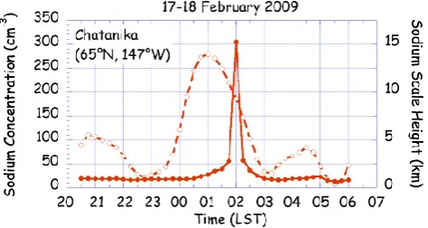
Fig. 5. Characteristics of bottomside of the sodium layer as a function of time (LST = UT−9 h) measured by resonance lidar at Chatanika, Alaska on the night of 17–18 February 2009. The sodium concentration averaged over the 76–77 km altitude range (dashed line with open circle) and the sodium scale height over the 75–78 km altitude range (solid line with full circle) are plotted.
Hecht et al., 1997, 2000; Collins and Smith, 2004; Xu et al., 2006).
Of particular interest is the spreading of the sodium layer on the bottomside that (serendipitously) coincides with the rocket-borne measurements when the 100 cm−3contour ap-pears below 76 km from 00:30 LST until 02:15 LST with a minimum altitude of 74.1 km at 02:00 LST and 02:15 LST. This behavior is evident in Figs. 3 and 4. In Fig. 3 the altitude separation of the 100 cm−3and 250 cm−3contours has a me-dian value of 0.9 km and reaches a maximum value of 4.4 km at 02:00 LST. This extension of the sodium layer below 78 km is clearly seen in the profile at 02:00 LST relative to the average profile in Fig. 4. In Fig. 5 we plot average sodium concentration and the bottomside scale height as functions of time. The average sodium concentration over the 76– 77 km altitude range reaches a maximum value of 279 cm−3 at 01:00 LST considerably larger than the local maxima of 110 cm−3at 20:45 LST and 84 cm−3at 04:30 LST. The bot-tomside scale height over a 3 km altitude range centered on the 184 cm−3sodium contour (at 76.5 km at 02:00 LST) has typical values of about 1 km when the 100 cm−3sodium con-tour is above 76 km. At 02:00 LST we find a bottomside scale height of 15.2±1.4 km over the 75–78 km altitude range.
4 Analysis
4.1 Motivation
[image:5.595.50.287.63.189.2]Based on the key observations (i.e., (i) appearance of a MIL with near-adiabatic lapse rate on the bottomside of the sodium layer, and (ii) simultaneous spreading of the sodium layer to unusually low altitudes) we analyze the observations in terms of wave-breaking, instability, and eddy diffusion to estimate the eddy diffusivity associated with the MIL. To il-lustrate our approach we plot the trajectory of the peak of
Fig. 6. Altitude of sodium concentration contours (alternate solid
and dashed lines) and mesospheric inversion layer peak (solid line with closed square) as a function of time measured by resonance and Rayleigh lidars respectively at Chatanika, Alaska on the night of 17–18 February 2009. The sodium concentration contours are labeled in cm−3.
scattering and concluded that the presence of the MILs coin-cided with instabilities and turbulence (Thomas et al., 1996). Liu and coworkers have conducted a series of numerical ex-periments to show that interactions between tides and gravity waves could result in gravity-wave breaking and the forma-tion of a MIL (Liu and Hagan, 1998; Liu et al., 2000; Liu and Meriwether, 2004). Salby and co-workers used lidar and satellite observations and models to show that the formation of MILs was consistent with breaking planetary waves (Salby et al., 2002). Meriwether and Gerrard (2004) have identified two subtypes of MILs. One type of MIL is found at higher altitudes (∼85 km and above) and are formed through inter-actions of gravity waves with large amplitude tidal waves. A second type of MIL is found at lower altitudes and are formed by dissipating planetary waves. In this study we ana-lyze the lidar observations in terms of vertical transport of a chemically active tracer to estimate the eddy diffusion associ-ated with the MIL. While we expect that the MIL at 74 km is formed by planetary waves, we do not attempt to directly de-termine the mechanism underlying the formation of the MIL (i.e., planetary-wave breaking or gravity-wave breaking).
From Figs. 3 and 5 we see that the sodium on the bot-tomside of the sodium layer disappears on the scale of tens of minutes. This is considerably longer than the chemi-cal time constants that are chemi-calculated for the sodium layer (e.g., Xu and Smith, 2003). Xu and Smith conducted an eigenvector-eigenvalue analysis of chemical timescales in the mesospheric sodium layer following the approach used by Prather (1994) in studying methane and in control theory since the 1960s (Gilbert, 1963). We have confirmed this behavior in the bottomside of the sodium layer using tem-perature and concentration profiles from the Thermosphere-Ionosphere-Mesosphere-Electrodynamics General Circula-tion Model (Roble and Ridley, 1994) and a sodium layer model (Plane et al., 1998). In mixing the atmosphere over several kilometers (e.g., between 75 and 78 km) the atomic sodium converges to the new mixed equilibrium in seconds. The longer sodium lifetime reflects the equilibrium of atomic sodium with other sodium species and background species (e.g., atomic oxygen, ozone, etc.) as they evolve. Liu et al. (2000) modeled the evolution of atomic oxygen associ-ated with the formation of a MIL and show features lasting several hours. Thus the atomic sodium remains in a fast equi-librium with the more slowly evolving background species and eventually disappears as these species disappear. 4.2 Estimation of eddy diffusion coefficient
We determine the value of the eddy diffusion coefficient fol-lowing the analysis by Hunten of vertical transport in the atmosphere (Hunten, 1975). Ignoring vertical velocity and molecular diffusion, we can express the vertical flux of a mi-nor constituent,φ, as,
φ= −K×na× df
dz (1)
whereKis the eddy diffusion coefficient,nais the concen-tration of the background atmosphere, andf (=n/na)is the mixing ratio of the tracer,n. The sodium lidar provides mea-surements ofn, while the Rayleigh lidar provides measure-ments of the relative concentration of the background atmo-sphere,ra, which can be normalized to 1 at the altitude of interest. Thus the expression for the vertical flux becomes,
φ= −K×
dn
dz−n dra
dz
(2) Using the scale height of a tracer with concentration increas-ing with height, H, and the background atmosphere with concentration decreasing with height,Ha, we can express the flux in terms of the scale heights as,
φ= −K×n×
1 H+
1 Ha
(3) Following Hunten, we estimate φby assuming that during the disappearance of the sodium, the diffusion is suppressed and the observed loss rate is the chemical loss rate. Thus when the turbulence is fully formed, and the sodium has the largest scale height (02:00 LST), the downward vertical flux rate balances the chemical loss rate, and we can express the flux gradient as,
dφ dz = −
n
τ (4)
whereτ is the loss time constant. Following Whiteway et al. (1995), we assume a single slab of uniform turbulence over layer thickness,L, and integrate Eq. (4) to yield the flux as,
φ= −n
τ ×L (5)
Finally we determineKfrom Eqs. (3) and (5) as, K=L
τ ×Heff (6)
where the effective scale height,Heff, is, 1
Heff
= 1
H+ 1 Ha
. (7)
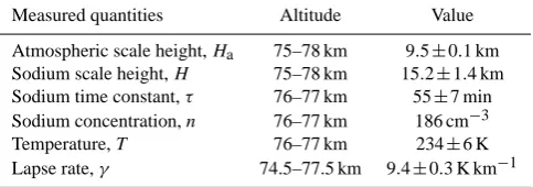
Measured quantities Altitude Value
Atmospheric scale height,Ha 75–78 km 9.5±0.1 km Sodium scale height,H 75–78 km 15.2±1.4 km Sodium time constant,τ 76–77 km 55±7 min Sodium concentration,n 76–77 km 186 cm−3
Temperature,T 76–77 km 234±6 K
Lapse rate,γ 74.5–77.5 km 9.4±0.3 K km−1
tabulate these values in Table 2 with a range determined from the uncertainty in the measurements reported in Table 1.
However, our analysis assumes that the observed lifetime of the sodium represents the chemical loss rate. This analysis is only correct if the atmosphere is at rest. The measured lifetime may be significantly shorter than the true lifetime of the layer due to advection. For a layer with horizontal scale length,Lh, and a vertical scale height,Hv, in the presence of winds with horizontal velocityVh, and vertical velocityVv, the observed lifetime,τobs, is related to the true lifetime,τ, as,
1 τobs
=1
τ± 1 τh
± 1
τv
(8) where τh (=Lh/Vh) and τh (=Hv/Vv) are the horizontal and vertical advection timescales respectively. Clearly the observed lifetime can be significantly greater or less than the true lifetime, and from Eq. (6) can yield an estimate of the eddy diffusion coefficient that is significantly biased. We estimate the true lifetime by considering the winds and sodium scale lengths and sizes. The luminous vapor trails released by the rocket yield horizontal wind measurements from 85 to 130 km (Lehmacher et al., 2011). The wind speeds near 85 km are approximately 50 m s−1. We assume wind speeds of 50 m s−1 at the altitude of the MIL (76– 77 km) and a horizontal scale length for the sodium en-hancement of 250 km. The 3.5 h oscillation of amplitude 0.9 km suggests vertical winds of amplitude 0.44 m s−1 as-sociated with a gravity wave. Analysis of gravity waves in the sodium layer indicate that the sodium displacement os-cillations are∼25 % larger than the wave displacement per-turbations and so we use this value as representative of the gravity wave winds (Collins and Smith, 2004). The ampli-tude of the wave (0.9 km) is less than the altiampli-tude spreading of the sodium (3 km). The measured sodium scale height is 15.2 km. Thus the horizontal advection timescale is 83 min and the vertical advection timescale is 576 min. We used these timescales to calculate a value of the true lifetime be-tween 31 and 225 min. Thus the value of the eddy diffusivity may be as low as 4.3×10²m2s−1and a downward sodium
4.3 Estimation of eddy dissipation rate
Following Weinstock (1978) we relate the eddy diffusion co-efficient,K, and the energy dissipation rate,ε, as,
ε= 1
0.81×
N2×K (9)
whereN is the Brunt-V¨ais¨al¨a frequency. We calculate the Brunt-V¨ais¨al¨a frequency as,
N2=g
T ×(0−γ ) (10)
whereg is the gravitational constant (9.6 m s−2), T is the temperature,0is the adiabatic lapse rate (9.5 K km−1), and γis the lapse rate. Using the values in Tables 1 and 2, we es-timate a value of the square of the Brunt-V¨ais¨al¨a frequency of 4.1×10⁻⁶s−2 (corresponding to a buoyancy period of 52 min) and an energy dissipation rate of 2.2 mW kg−1. The uncertainty in the measured near-adiabatic lapse rate results in a large uncertainty in the square of the Brunt-V¨ais¨al¨a frequency (0–17×10−6s−2)and contributes to the large uncertainty in the estimated eddy dissipation rate (0– 11 mW kg−1).
5 Discussion
5.1 General structure of stratosphere and mesosphere
[image:7.595.49.291.120.205.2]Table 2. Derived eddy diffusion quantities based on lidar observations of MIL and sodium layer on 17–18 February 2009 at Chatanika
(65◦N, 147◦W).
Derived eddy quantities Value Range
Effective scale height,Heff 5.8 km 5.6–6.1 km Square of Brunt-V¨ais¨al¨a frequency,N2 4.1×10⁻⁶s−2 0–17×10−6s−2 Eddy diffusion coefficienta,K 1.8×10³m2s−1 1.5–2.1×10³m2s−1 Eddy sodium fluxa,φ 5.6×10⁷(atoms m−2)s−1 5.0–6.5×10⁷(atoms m−2)s−1 Eddy diffusion coefficientb,K 4.3×10²m2s−1 3.7–5.2×10²m2s−1 Eddy sodium fluxb,φ 1.4×10⁷(atoms m−2)s−1 1.2–1.6×10⁷(atoms m−2)s−1 Energy dissipation rateb,ε 2.2 mW kg−1 0–11 mW kg−1
aUnder assumption of zero wind;bunder assumption of nonzero winds
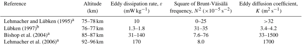
Table 3. Measured eddy dissipation rates and diffusion coefficients in the upper mesosphere and lower thermosphere.
Reference Altitude Eddy dissipation rate,ε Square of Brunt-V¨ais¨al¨a Eddy diffusion coefficient, (km) (mW kg−1) frequency,N2(×10−5s−2) K(m2s−1)
Lehmacher and L¨ubken (1995)a 75–78 km 10 0–25 >32
L¨ubken (1997)b 76–77 km 1.3–1.8 31–35 3.4–4.2
Bishop et al. (2004)a 85–87 km 31–140 7.6–76 33–1500
Lehmacher et al. (2006)a 92–96 km 170 8.0 1700
aSingle rocket-borne measurement;bseasonal averages of 12 rocket-borne measurements
vortex was anomalously cold and lead to the formation of an elevated stratopause in February 2009. The formation of the elevated stratopause has been documented in zonal mean temperature measurements at 70◦N (Manney et al., 2009). The lower stratospheric vortex remained weak through the end of March 2009.
Despite the disturbed condition of the stratosphere and lower mesosphere, the structure of the mesospheric sodium layer on the night of 17–18 February 2009 was typical for this time of year at Chatanika as reported by Collins and Smith (2004) and as confirmed by both ongoing measure-ments at Chatanika and measuremeasure-ments made during Febru-ary 2009 in support of the Turbopause experiment. The val-ues of the sodium layer parameters and the asymmetry of the layer were consistent our understanding of the chemical equilibrium of the sodium layer (e.g., Plane, 2004), and with the latitudinal variation of the sodium layer that have been reported from other sites around the world (e.g., Yi et al., 2009).
5.2 Eddy diffusion and dissipation
The observations in this study have allowed us analyze tur-bulence in the upper mesosphere by first determining the eddy diffusion coefficient and then determining the eddy dissipation rate. Experiments that employ spectral analysis of small-scale high-frequency density fluctuations, expan-sion of luminous vapor trails use analyses that determine
[image:8.595.50.543.267.344.2]atmosphere varied considerably with the processes that cause the turbulence. The lidar measurements in the Turbopause experiment are made in the presence of a mature MIL where the lapse rates are similar to those reported by Lehmacher and L¨ubken (1995) and persist for several hours. Bishop et al. (2004) suggest that their measurements of large eddy dif-fusion coefficient reflect the role of large vortices generated by tides in creating vortex role instabilities. Similarly the measurements of Lehmacher et al. (2006) of large dissipa-tion rates above 90 km may represent the generadissipa-tion of tur-bulence associated with interaction between large amplitude gravity-waves and/or tides associated with the formation of a high altitude MIL (Meriwether and Gerrard, 2004).
6 Summary and conclusions
Simultaneous Rayleigh and resonance lidar measurements made during the Turbopause experiment have allowed us conduct a detailed investigation of a MIL that formed near the lower edge of the sodium layer. The lidar experiments differed from previous experiments at Chatanika in two dis-tinct ways; the Rayleigh lidar incorporated simultaneous rocket-borne temperature measurements in the upper meso-sphere to yield more accurate temperature measurements above 60 km, the resonance lidar incorporated a larger tele-scope than previously used to allow more precise measure-ments of the sodium layer.
The thermal structure of the stratosphere and mesosphere is disrupted during a major stratospheric warming that re-sulted in disruption of the stratospheric vortex with a cold stratopause present throughout February 2009. The general structure of the mesospheric sodium layer is typical of that observed at Chatanika in February.
However, the observations also revealed the downward transport of sodium to unusually low altitudes coinciding with the presence of a MIL. The MIL had large amplitude, near adiabatic lapse rate, and was present for over 6 h. The formation and downward motion of the MIL was accompa-nied by the extension of the sodium layer to unusually low latitudes over a 2–3 h period. The sodium appears to have been entrained in the MIL. Using simple continuity argu-ments we have modeled the vertical motion of the sodium as due to downward diffusion in the presence of the MIL. Even allowing for the presence of strong winds, our analysis yields an estimate of the eddy diffusion coefficient (430 m2s−1) that is significantly larger that that reported for mean win-tertime values by L¨ubken (1997). Our estimates of the eddy diffusion coefficient are similar to values found in a super-adiabatic layer near 75 km (Lehmacher and L¨ubken, 1995) and in a region of static instability near 85 km (Bishop et
Our observations and analysis, based on naturally occur-ring variations in mesospheric temperatures and the sodium layer (rather than artificial releases or measurement of small-scale density fluctuations), confirm that there is significant eddy diffusion associated with convectively unstable regions of MILs in the upper mesosphere.
Acknowledgements. The authors thank Brita Irving, Agatha Light,
Kate Schaefer, and Brentha Thurairajah for assistance with the li-dar observations. The authors thank the staff at Poker Flat Research Range (PFRR) for their ongoing support of the lidar observations at PFRR. The authors thank Raymond Roble of the National Cen-ter for Atmospheric Research (NCAR) for providing the NCAR model results. The 41 inch telescope used in this study was de-ployed at PFRR with support from Chester Gardner of the Univer-sity of Illinois and the National Science Foundation (NSF). The au-thors thank Annraoi de Paor of the National University of Ireland for helpful discussions. The authors thank two anonymous referees for their review of the paper. This work was carried out with support from National Aeronautics and Space Administration (NASA) un-der grants NNX08AC57G and NNX07AJ99G and from NSF unun-der grants ATM-0122995 and AGS-1007539. PFRR is a rocket range operated by the Geophysical Institute of the University of Alaska Fairbanks with support from NASA.
Topical Editor C. Jacobi thanks two anonymous referees for their help in evaluating this paper.
References
Bishop, R. L., Larsen, M. F., Hecht, J. H., Liu, A. Z., and Gard-ner, C. S.: TOMEX: Mesospheric and lower thermospheric dif-fusivities and instability layers, J. Geophys. Res., 109, D02S03, doi:10.1029/2002JD003079, 2004.
Collins, R. L. and Smith, R. W.: Evidence of damping and over-turning of gravity waves in the arctic mesosphere: Na lidar and OH temperature observations, J. Atmos. Solar-Terr. Phys., 66, 867–879, 2004.
Collins, R. L., Hallinan, T. J., Smith, R. W., and Hernandez, G.: Li-dar observations of a large high-altitude sporadic Na layer during active aurora, Geophys. Res. Lett., 23, 3655–3658, 1996. Cutler, L. J., Collins, R. L., Mizutani, K., and Itabe, T.: Rayleigh
lidar observations of mesospheric inversion layers at Poker Flat, Alaska (65◦N, 147◦W), Geophys. Res. Lett., 28, 1467–1470, 2001.
Fritts, D. C. and Alexander, M. J.: Gravity wave dynamics and effects in the middle atmosphere, Rev. Geophys., 41, 1003, doi:10.1029/2001RG000106, 2003.
Fritts, D. C., Bizon, C., Werne, J. A., and Meyer, C. K.: Lay-ering accompanying turbulence generation due to shear insta-bility and gravity-wave breaking, J. Geophys. Res., 108, 8452, doi:10.1029/2002JD002406, 2003.
Illi-nois, 1. Seasonal and nocturnal variations, J. Geophys. Res., 91, 13659–13673, 1986.
Gilbert, E. G.: Controllability and Observability in Multivariable Control Systems, SIAM J. Cont., A, 2, 128–151, 1963.
Hecht, J. H.: Instability layers and airglow imaging, Rev. Geophys., 42, RG1001, doi:10.1029/2003RG000131, 2004.
Hecht, J. H., Waltersheid, R. L., Fritts, D. C., Isler, J. R., Senft, D. C., Gardner, C. S., and Franke, S. J.: Wave breaking signatures in OH airglow and sodium densities and temperatures, 1. Airglow imaging, Na lidar, and MF radar observations, J. Geophys. Res., 102, 6655–6668, 1997.
Hecht, J. H., Fricke-Begemann, C., Walterscheid, R. L., and H¨offner, J.: Observations of the breakdown of an atmospheric gravity wave near the cold summer mesopause at 54N, Geophys. Res. Lett., 27, 879–882, doi:10.1029/1999GL010792, 2000. Hecht, J. H., Liu, A. Z., Bishop, R. L., Clemmons, J. H., Gardner,
C. S., Larsen, M. F., Roble, R. G., Swenson, G. R., and Wal-terscheid, R. L.: An overview of observations of unstable lay-ers during the Turbulent Oxygen Mixing Experiment (TOMEX), J. Geophys. Res., 109, D02S01, doi:10.1029/2002JD003123, 2004.
Hunten, D. M.: Vertical transport in atmospheres, in: Atmospheres of Earth and Planets, edited by: McCormac, B. M., 59–72, Rei-del, Dordrecht, 1975.
Lehmacher, G. and L¨ubken, F.-J.: Simultaneous observation of con-vective adjustment and turbulence generation in the mesosphere, Geophys. Res. Lett., 22, 2477–2480, 1995.
Lehmacher, G. A., Croskey, C. L., Mitchell, J. D., Friedrich, M., L¨ubken, F.-J., Rapp, M., Kudeki, E., and Fritts, D. C.: In-tense turbulence observed above a mesospheric temperature in-version at equatorial latitude, Geophys. Res. Lett., 33, L08808, doi:10.1029/2005GL024345, 2006.
Lehmacher, G. A., Scott, T. D., Larsen, M. F., Bil´en, S., Croskey, C. L., Mitchell, J. D., Rapp, M., L¨ubken, F.-J., and Collins, R. L.: The Turbopause experiment: atmospheric stability and turbulent structure spanning the turbopause altitude, Ann. Geophys., in re-view, 2011.
Liu, H.-L. and Hagan, M. E.: Local heating/cooling of the meso-sphere due to gravity wave and tidal coupling, Geophys. Res. Lett., 25, 2941–2944, 1998.
Liu, H.-L. and Meriwether, J. W.: Analysis of a temperature in-version event in the lower mesosphere, J. Geophys. Res., 109, D02S07, doi:10.1029/2002JD003026, 2004.
Liu, H.-L., Hagan, M., and Roble, R.: Local mean state changes due to gravity wave breaking modulated by the diurnal tide, J. Geophys. Res., 105, 12381–12396, 2000.
L¨ubken, F.-J.: Seasonal variation of turbulent energy dissipation rates at high latitudes as determined by in situ measurements of neutral density fluctuations, J. Geophys. Res., 102, 13441– 13456, 1997.
Manney, G. L., Schwartz, M. J., Kr¨uger, K., Santee, M. L., Paw-son, S., Lee, J. N., Daffer, W. H., Fuller, R. A., and Livesey, N. J.: Aura Microwave Limb Sounder observations of dy-namics and transport during the record-breaking 2009 Arctic stratospheric major warming, Geophys. Res. Lett., 36, L12815, doi:10.1029/2009GL038586, 2009.
Meriwether, J. W. and Gerrard, A. J.: Mesosphere inversion layers and stratosphere temperature enhancements, Rev. Geophys., 42, RG3003, doi:10.1029/2003RG000133, 2004.
Plane, J. M. C.: A time-resolved model of the mesospheric Na layer: constraints on the meteor input function, Atmos. Chem. Phys., 4, 627–638, doi:10.5194/acp-4-627-2004, 2004.
Plane, J., Cox, R., Qian, J., Pfenninger, W., Papen, G., Gardner, C., and Espy, P.: Mesospheric Na layer at extreme high latitudes in summer, J. Geophys. Res., 103, 6381–6389, 1998.
Prather, M. J.: Lifetimes and eigenstates in atmospheric chemistry, Geophys. Res. Lett., 21, 801–804, 1994.
Randel, W., Udelhofen, P., Fleming, E., Geller, M., Gelman, M., Hamilton, K., Karoly, D., Ortland, D., Pawson, S., Swinbank, R., Wu, F., Baldwin, M., Chanin, M.-L., Keckhut, P., Labitzke, K., Remsberg, E., Simmons, A., and Wu, D.: The SPARC inter-comparison of middle- atmosphere climatologies, J. Climate, 17, 986–1003, 2004.
Roble, R. G. and Ridley, E. C.: A thermosphere-ionosphere-electrodynamics general circulation model (TIME-GCM): Equinox solar cycle minimum simulation (30–500 km), Geo-phys. Res. Lett., 21, 417–420, 1994.
Salby, M., Sassi, F., Callaghan, P., Wu, D., Keckhut, P., and Hauchecorne, A.: Mesospheric inversions and their relation-ship to planetary wave structure, J. Geophys. Res., 107, D4, doi:10.1029/2001JD000756, 2002.
Schoeberl, M., Strobel, D., and Apruzese, J.: A Numerical Model of Gravity Wave Breaking and Stress in the Mesosphere, J. Geo-phys. Res., 88, 5249–5259, 1983.
Siskind, D. E., Eckermann, S. D., Summers, M. E. (Eds.): Science across the stratopause, Geophysical Monograph 123, American Geophysical Union, Washington, 2000.
SPARC: SPARC Intercomparison of Middle Atmosphere Clima-tologies, SPARC Rep. 3, 96 pp., 2002.
Thomas, L., Marsh, A., Wareing, D., Astin, I., and Chandra, H.: VHF echoes from the midlatitude mesosphere and the thermal structure observed by lidar, J. Geophys. Res., 101, 12867–12877, 1996.
Thurairajah, B., Collins, R. L., and Mizutani, K.: Multi-Year tem-perature measurements of the middle atmosphere at Chatanika, Alaska (65◦N, 147◦W), Earth Planets Space, 61, 755–764, 2009.
Thurairajah, B., Collins, R. L., Harvey, V. L., Lieberman, R. S., Gerding, M., Mizutani, K., and Livingston, J. M.: Gravity wave activity in the Arctic stratosphere and meso-sphere during the 2007–2008 and 2008–2009 stratospheric sudden warming events, J. Geophys. Res., 115, D00N06, doi:10.1029/2010JD014125, 2010a.
Thurairajah, B., Collins, R. L., Harvey, V. L., Lieberman, R. S., and Mizutani, K.: Rayleigh lidar observations of reduced gravity wave activity during the formation of an elevated stratopause in 2004 at Chatanika, Alaska (65◦N, 147◦W), J. Geophys. Res., 115, D13109, doi:10.1029/2009JD013036, 2010b.
Vlasov, M. N. and Kelley, M. C.: Crucial discrepancy in the bal-ance between extreme ultraviolet solar radiation and ion densities given by the international reference ionosphere model, J. Geo-phys. Res., 115, A08317, doi:10.1029/2009JA015103, 2010. Weinstock, J.: Vertical Turbulent Diffusion in a Stably
Strati-fied Fluid, J. Atmos. Sci., 35, 1022–1027, doi:10.1175/1520-0469(1978)035<1022:VTDIAS>2.0.CO;2, 1978.