No diffusion in solid, no concentration gradients in liquid

A reminder: the lever rule

Material balance









S S L

A

S S L L B

n n x n x

n n x n x

          L (1)

Solution of (1) is trivial:





_

_

L L L

S B A B

S L

S L

n x

n n x n

n x n x n x

n

x x D D

x x



A  B  B

 

  

  (2)

where 1 1









S L

S L L S L L S S L S L S

S L

x x

D x x x x x x x x x

x x

 

         x x x





_

_

S S S

L B A A

S L

S L

x n

n n n x

x n n x n x

n

x x D D

x x          

B A B

(3)

Let us use (2) and (3) for finding the nL nS ratio:

















S

B A B

S

L S

B A B A B

L

S L

A B B

A B B

A B

n n n x

n n n x n n

n D

n n x n

n D n n x n x

n n

 

   

 

  L

x x x



  



It is worth reminding that the distribution coefficient (a.k.a. partition coefficient) is defined as S L

Not only mole fractions of the second component in the solid and liquid phases can be used, but weight fractions and concentrations as well. Needless to clarify that the value of distribution coefficient depends on units chosen.

No diffusion in solid, no concentration gradients in liquid

 

Before After

L S L

AdzC AdzC A L z dz dC

 

If dz L z (recall that this condition is not valid when solidification is almost finished), then

 

L S

dzC dzC  Lz dCL

L





C C dz Lz dC

Let us realize that CS kCLCLCS CL1k:

 

 

1 L L

dC k dz

C L z

 



 

  _{ }

       

0 0

0

1

1 1

L

L

C z z L z z z z z z

L

z z z

C z

dC k dz d L z d L z

k k

C L z L z L

   

  



 

     

 









0 z

 

 

       

0

1 0

ln 1 ln 1 ln ln

0

k L

z L

C

C z L z L z

k L z k

C z L L



   

     _{ } 

 

1 0

k

L L z

C C L

 

 

 _{ }

  (4)

1 0

k

S L L z

C kC kC L

 

 

   

  (5)

Remember about the assumptions under which (4) and (5) were derived: 1. Uniform liquid composition

2. A plane solid/liquid interface

3. Negligible diffusion in the solid state 4. k = const

5. Equal solid and liquid densities (i.e. equal molar volumes)

Assumption 5 is not needed if concentration C is replaced with weight fraction and if z L is replaced with the weight fraction of alloy already solidified.

No diffusion in solid, diffusional and convectional mixing in

liquid

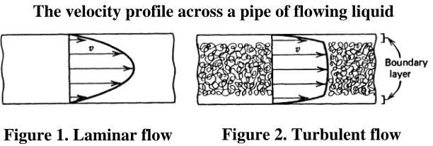
Convection in the liquid portion of a solidifying alloy tends to produce a uniform liquid composition. Since natural convection is difficult to eliminate from liquid metal alloys because of their low viscosity and high density, one expects a uniform liquid composition to be obtained. However, there is a fundamental characteristic of fluid flow that prevents this. When a fluid flows near a solid surface, the velocity of the fluid at the surface is always equal to zero (no-slip condition). If a fluid is passed down a tube at a low velocity as shown in Figure 1, the fluid flows parallel to the pipe wall at all points and is termed laminar flow.

The velocity profile across a pipe of flowing liquid

Figure 1. Laminar flow Figure 2. Turbulent flow

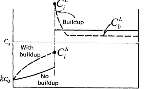
suggests, however, that the velocity must always drop to zero at the wall. Hence, a thin boundary layer of laminar flowing fluid is always present at the wall. Such a boundary layer is always present in the liquid at the solid–liquid interface, and it inhibits a uniform liquid composition. If solute is being rejected from the solid into the liquid at the solid–liquid interface, then in order to obtain a uniform liquid composition this solute must be transported swiftly throughout the liquid. Two transport mechanisms are available to mix this solute into the liquid: diffusion and convection. Of these two, diffusion is a much slower mechanism. In the boundary layer at the interface, there can be no convective transport normal to the interface because of the laminar flow parallel to the interface. Solute can only be transported through the boundary layer into the liquid mixed by convection by the slow mechanism of diffusion. Consequently, a buildup of solute is obtained in the boundary layer region as is shown by the dashed curve in Figure 3.

Figure 3 The presence of build-up affects the composition of solidifying substance

Beyond the boundary layer, the bulk liquid composition is uniform at the value due to

mixing. Since local equilibrium takes place at the interface, we have (b and i are used for designating bulk and interface, correspondingly). The solute buildup causes to rise rapidly and, hence, must also rise rapidly. Therefore, the solid composition rises more

rapidly than for the case of no buildup, as illustrated in

L b

C

L i

C

S i

C kC_iL

S i

C

Figure 3.

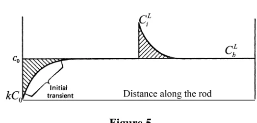
diffusion increases until eventually a balance is obtained between the input and output to the boundary layer region. At this point the buildup stops rising such that the ratio C_iL C_bL becomes constant. The region over which the buildup occurs is called the initial transient.

Figure 4 Solute build-up evolution

Let us define effective distribution coefficient (sometimes it is called effective partition coefficient:

eff

S S

i i

L L

b b

x C k

x C

 

After completion of the initial transient, is constant. Its value tells much about the effect of

liquid mixing upon the solute profile that is frozen into the solid.

eff

k

Case 1: k

= 1

Figure 5

Since . The buildup carries the solid composition all the way up to the original

com ixing is not sufficient to raise above . This result is obtained

for the case of very little or no mixing.

eff 1

k  , position

S L

i b

C C

0

2: ke

k

Case

In this case

eff

S S

S

i i

L L

i b

C C

C

k k

C C C

    _L

which immediately gives , which means there is no buildup. Hence, there is uniform

ase 3 (intermediate): k < k

< 1

L L

i b

C C

liquid composition.

C

The initial transient is followed by a gradually rising solid composition similar to Case 2, but at a higher level of composition.

Derivation of the unidirectional growth equation

In this section, we are concerned with the steady state, which occurs after initial transient. The

tration of solute in the solid phase must be equal to its initial o solute cannot be derivation corresponds to the situation shown in Figure 5, i.e. to the case keff 1. It is clear that

if a rod is infinitely long, the concen

concentration in the melt. Otherwise, the material balance with respect t satisfied.

the flux of solute.

(i.e. in the positive direction of the axis z) and holds a reference surface that is used for measuring

Since the interface moves into the rema quid phase, the observer sees a flow of liquid passing through the reference surface. This flow is directed in his/her face, i.e. in the negative direction. Clearly, there are two fluxes:

ining li

total int diff diff

J J J  vCJ

where J_int is the flux caused by the interface motion, and J_diff is the diffusion-induced flux.





total

z

vC J J

C C

t

  



 _{  }  

 

diff

2

z z z

C

v D

  

   (6)

teady-state means that the concentration of lute in liquid does not depend on , which allows rite

t

S so

us to w (6) as:

2

2 0

d C v dC

dz D dz  (7)

(7) suggests that the solution of this differential equation should be sought within the class of exponential functions:

which is known as unidirectional growth equation. The appearance of

  exp 

C z  A B z

where  0, indeed.

  ₀

C z  C A

z0C_eqL C₀Bexp 0 C₀  B B C_eqL C₀ C

  ₀





C z C  C C z (8)

Let us differentiate (8):





dC

C C z

dz     (9)

Let us differentiate (9):





2

2

eq 0

2 exp

L

d C

C C z

dz    

0) in (7) gives:

(10)

Substitution of (9) and (1









eq 0 exp eq 0 exp z 0

L v L

C C z C C

D

  

  

v D

  

 





0 eq 0 exp

L v

C z C C C z

D

 

   _ _

  (11)

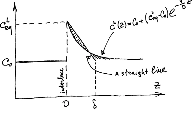
llow me to remind you that (11) is the solution of (7). This solution can be used for figuring out what the equivalent boundary layer is.

A

Let us calculate an overall excess of solute in liquid with respect to its initial concentration:

(12)

Substitution of (11) in (12) gives:

 





0

L

C z C dz































0 eq 0 0 eq 0

0 0

eq 0

0

eq 0 eq 0 eq 0

0

exp exp

exp

exp 0 1

L L

L

z

L L

z

v v

C C C z C dz C C z dz

D D

D v v

C C z d z

v D D

D v D

C C z C C C C

v D v

 







 _{ } _ _  _{ } _ 

   

 _{ }  _{ }

 

     

  _ _{ } _{ } _

   

 

     

  _ _ _ _   _ _   

 

   







L D

v

If the actual function is replaced with a straight line in such a fashion that two differently hatched areas in Figure 6 are equal, then









2

v

1

L L

C C D  C C 

2D v

 

Roughly, we can say

diffusion

z 

convectionz 