Effects of dispersion on the inference of metal texture from S0 plate mode measurements. Part I. Evaluation of dispersion correction methods

Ames Laboratory Publications

Ames Laboratory

3-1992

Effects of dispersion on the inference of metal

texture from S0 plate mode measurements. Part I.

Evaluation of dispersion correction methods

Yan Li

Iowa State University

R. Bruce Thompson

Iowa State University

Follow this and additional works at:

http://lib.dr.iastate.edu/ameslab_pubs

Part of the

Engineering Mechanics Commons

,

Materials Science and Engineering Commons

,

and the

Structures and Materials Commons

The complete bibliographic information for this item can be found at

http://lib.dr.iastate.edu/

ameslab_pubs/11

. For information on how to cite this item, please visit

http://lib.dr.iastate.edu/

howtocite.html

.

Effects of dispersion on the inference of metal texture from S0 plate mode

measurements. Part I. Evaluation of dispersion correction methods

Abstract

Ultrasonic

S

waves (fundamental symmetric Lamb modes) are being considered in several laboratories for

the nondestructive characterization of the texture (preferred grain orientation) and formability of metal

sheets and plates. In a typical experimental setup, the velocities of the

S

waves are measured as a function of

wave propagation angle with respect to the rolling direction of the plate. However, the

S

waves are known to

be dispersive, and that dispersion must be considered in order to isolate the small, texture‐induced shifts in

the

S

wave velocity. Currently, there are two approximate dispersion correction methods, one proposed by

Thompson

et al

.

and the other introduced by Hirao and Fukuoka.

In this paper, these two methods will be

evaluated using an exact theory for wave propagation in orthotropic plates. Through the evaluation, the limits

of the current texture measurement techniques are established. It is found that when plate thickness to

wavelength ratio is less than 0.15, both Thompson’s and Hirao’s methods work satisfactorily. When the

thickness to wavelength ratio exceeds 0.3, neither Thompson’s nor Hirao’s dispersion correction method

provides adequate corrections for the current texture measurement techniques. Within the range of 0.15–0.3,

Thompson’s method is recommended for weakly anisotropic sheets and plates and Hirao’s method may be

more appropriate for some strongly anisotropic cases.

Keywords

metals, plates, wave propagation, anisotropy, ultrasonic testing, texture, refraction

Disciplines

Engineering Mechanics | Engineering Science and Materials | Materials Science and Engineering | Structures

and Materials

Comments

This article is from

Journal of the Acoustic Society of America

91, no. 3 (1992): 1298–1309, doi:

10.1121/

1.402512

.

Effects of dispersion on the inference of metal texture from S0 plate

mode measurements. Part I. Evaluation of dispersion correction

methods

Yan Li and R. Bruce Thompson

Ames Laboratory, Iowa State University, Ames, Iowa 50011

(Received 3 June 1990; revised 17 May 1991; accepted 1 November 1991 )

Ultrasonic So waves (fundamental symmetric Lamb modes) are being considered in several laboratories for the nondestructive characterization of the texture (preferred grain orientation) and formability of metal sheets and plates. In a typical experimental setup, the velocities of the So waves are measured as a function of wave propagation angle with respect to the rolling direction of the plate. However, the So waves are known to be dispersive, and that dispersion

must be considered in order to isolate the small, texture-induced shifts in the So wave velocity.

Currently, there are two approximate dispersion correction methods, one proposed by Thompson et al. [Met. Trans. A 20, 2431 (1989) ] and the other introduced by Hirao and Fukuoka [J. Acoust. Soc. Am. 85, 2311 (1989) ]. In this paper, these two methods will be evaluated using an exact theory for wave propagation in orthotropic plates. Through the evaluation, the limits of the current texture measurement techniques are established. It is found that when plate thickness to wavelength ratio is less than 0.15, both Thompson's and Hirao's methods work satisfactorily. When the thickness to wavelength ratio exceeds 0.3, neither Thompson's nor Hirao's dispersion correction method provides adequate corrections for the current texture measurement techniques. Within the range of 0.15-0.3, Thompson's method is recommended for weakly anisotropic sheets and plates and Hirao's method may be more appropriate for some strongly anisotropic cases.

PACS numbers: 43.20.Ks, 43.35.Cg, 43.40.Le, 43.20.Bi

INTRODUCTION

Texture is the nonrandom orientation of crystallites in a

polycrystalline aggregate, often induced by manufacturing processes such as rolling and drawing. The texture is charac-

terized by a set of dimensionless parameters Wlmn, called

orientation distribution coefficients (ODCs). These coeffi-

cients, whose detailed definitions can be found in Refs. 1 and

2, specify the relative weights of generalized spherical har-

monics in a series representation of the orientation distribu- tion function (the probability that a grain has a particular orientation). Knowledge of texture information is particu- larly important in making formability predictions, i.e., pre- dictions of the ability of a sheet to be converted to a complex

shape by a deep drawing operation. For materials made of

cubic crystallites, such as A1 (fcc), Cu (fcc), and Fe (bcc), the most important ODCs in formability analysis are W4oo,

W42o, and W44o. Physically, W42o and W44o relate to the tendency of a metal sheet to form two and four ears, respec- tively, upon deep drawing. Here W4oo relates to overall ca-

pacity

to withstand

deep

drawing.

3 Typical

values

of these

ODCs are on the other of 10- 3.

Traditionally, these ODCs are obtained through x-ray or neutron diffraction techniques. In recent years, however,

it has been shown that ultrasonic waves can be utilized to

provide a nondestructive estimation of the texture of cubic

polycrystals.

4-9

The texture

generally

induces

a weak

elastic

be easily interpreted in terms of the theory of guided modes.

In contrast to the neutron or x-ray diffraction techniques,

the ultrasonic techniques cannot obtain sufficient informa- tion to fully characterize the texture. However, they do pro-

vide information about W4oo, W42o, and W44o, the ODCs most important in formability analysis.

Because of the richness of information that they can

obtain, the x-ray and neutron diffraction techniques are gen-

erally preferred for laboratory studies of such phenomena as the evolution of texture during deformation of a material.

However, there is also a need for simple nondestructive mea-

surement techniques for field applications. The functions

needed include both obtaining feedback information for pro-

cess control by the primary manufacturers of the sheet and inspecting incoming material for quality control by the com-

ponent

fabricator.

Here the neutron

techniques

are impracti-

intensity.

The x-ray techniques

are being

employed.

•ø'•

12-18 ture in metal sheet in the last five years.

The ultrasonic techniques have utilized electromagnet- ic-acoustic transducers (EMATs)•9 to excite Lamb waves

propagating in the plane of the sheet with no need for a cou- plant. Since only three constants (W4oo, W42o, and W44o )

define the elastic anisotropy in the most commonly used ap-

proximations, only three velocities need to be measured,

typically those of So modes propagating at 0 ø, 45 ø, and 90 ø with respect to the metal sheet. To minimize both the effects of dispersion on the velocity and the sensitivity of the mea- surement to the distance between the EMATs and the plate, the wavelength is generally chosen to be somewhat greater than the plate thickness. Nevertheless, because the texture- induced velocity shifts are small, the experimental data must be corrected for the dispersion if accurate predictions of the ODCs are to be made. The theory for wave propagation in anisotropic media is well known. However, since the anisot- ropy is unknown at the time of measurement, use of the full theory in interpreting data is cumbersome. Because of this fact, and the smallness of the dispersion at long wavelengths, the correction is generally made on the basis of an isotropic theory. The purpose of this paper is to examine the adequacy of the currently used approximate correction techniques with the exact theory being utilized to generate simulated

data.

There are two aspects of the influence of dispersion of the So waves on the velocity measurements. First, both the phase velocity and the group velocity are frequency depen- dent. Two dispersion correction methods have been pro-

posed by Thompson et al. 9 and Hirao and Fukuoka 2ø to

remove the frequency dependence. In this paper, these two dispersion correction methods will be evaluated assuming perfect measurements of phase velocity. Another aspect of dispersion is the pulse distortion phenomenon; i.e., a pulse of a dispersive wave changes its shape and spreads out as it propagates. In Part II of this paper we discuss the influence of the pulse distortion on the accuracy of phase velocity mea-

surements.

Several years ago, Thompson et al. • and Lee et al. •

developed a theory that relates the aforementioned ODCs of textured sheets to the So wave speeds in three different direc- tions (0 ø, 45 ø, and 90 ø) with respect to the rolling direction. This theory assumes the ratio of sheet thickness to wave- length to be small. In this limit, the velocity of the So wave in a specific propagation direction asymptotically approaches a constant value, Vlim, and dispersion can be ignored. Upon comparison of experimental predictions of the ODCs based on this theory with the results from independent x-ray or neutron diffraction techniques, satisfactory agreement was found for W420 and W440, but not for W400. In those mea- surements, the ratio of thickness to wavelength was about

0.1. Recently, Thompson et al. 9 modified the theory and

included dispersion correction in the calculation of the ODCs. In the modified theory, the dispersion correction is made on the basis of dispersion curves of the So waves in the corresponding isotropic materials. It is assumed that the ra-

tio rp/Vli m is not altered

significantly

by the presence

of

velocity measured at a specific frequency and Vii m is the long wavelength limit of the So wave phase velocity. Hirao and

Fukuoka :ø have proposed another method, which takes dis-

persion effects into account by making a Taylor series expan- sion of the dispersion curves of the So mode propagating in weakly orthotropic media. In the expansion, only the first- order dispersion effects are retained.

The basis of our evaluation of the approximate disper-

sion correction methods is the exact theoretical equations recently developed for wave propagation in plates with orth-

otropic symmetry. •3-26 The equations that express the de-

pendence of wave propagation velocity upon texture param- eters are very complex and a simple technique has not been developed to compute the ODCs from given wave velocities on the basis of these exact equations. These equations, how- ever, can serve as an exact reference solution. In this paper, we will use the exact solution for the So wave propagation in orthotropic plates to simulate experimental data and then use those data to test the accuracy of the two approximate dispersion correction methods.

One semantic difficulty should be resolved before pro- ceeding. In the metallurgical community, the terms "sheet" and "plate" have connotations of different thicknesses, with the former appropriate to thicknesses on the order of a milli- meter to which the ultrasonic approach has been most exten- sively applied. In the ultrasonic literature, the term "plate" is generally used to describe a solid medium having parallel surfaces, independent of thickness. In the remainder of this paper, the latter convention will be employed. However, in considering metallurgical applications, the "sheets" should

be understood to be included.

I. GENERAL THEORY FOR WAVE PROPAGATION IN ORTHOTROPIC FREE PLATES

The authors of the present paper •3'•4 and Nayfeh and Chimenti 25'•6 have recently developed and reported the ana-

lytical dispersion equations for wave propagation in ortho- tropic or monoclinic free plates. For detailed derivation and discussions, the readers are encouraged to refer to these ref- erences. Here only the equations necessary to make this pa- per self-contained will be presented.

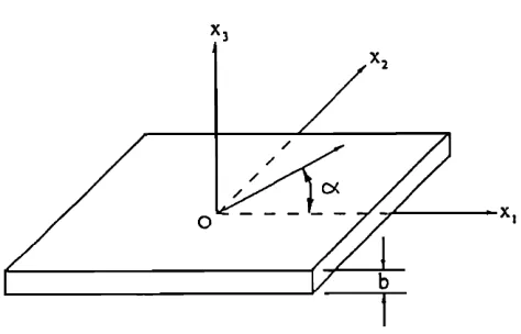
Consider the coordinate system shown in Fig. 1. Let us first make the following dimensionless definitions:

K 1 = K cos

2 a, K 2 = K sin

2 a, K = [ (b/•') k ]2,

666

-•-

r• (i - 1,2,3),

where b is the plate thickness, p is the density, C• are the

elastic constants of plate material, a is the wave propagation angle with respect to the rolling direction, k is the wave vec- tor in the propagation direction, co is the angular frequency

X 3

X I

FIG. 1. Definition of coordinates.

of the propagating wave, and r i are the eigenvalues of the associated Christoffel equations for plane wave propagation.

For a general elastic, homogeneous orthotropic free

plate whose rolling, transverse, and normal directions coin-

cide with the X2, X2, and X3 axes, as shown in Fig. 1, the dispersion equation for symmetric modes propagating at 0 ø

is

Q, {tan[ (z'/2)x/• ] }-2

- Q• {tan[ (z'/2)•3 ] }-2 = o,

Q(X,Y) = Xfr (C, 3X-- C,,K + C66

W')[

C33

C55

r

(1)

_ql_

(ell C33

-- C13

C55

-- C•3)g-- C33

C66

W],

and R2, R 3 are roots of the following equation for K3:

(Cll g _ql_ C55K 3 _ C66 W')(W55K _ql_ C33K 3 _ C66 W)

-- (C,3 + C55 )2K3K= 0.

The corresponding dispersion equation for symmetric modes propagating at 45 ø is (generalized Rayleigh-Lamb wave equation in orthotropic media)

P• tan(•x•)

-2+P

2

X [tan(-•xR/•-2)]-2+P3

tan(•xR•3)

-2--0,

(2)

where P• = P(R 2 ,R2,R 3 ), P2 = P(R2,R3,R2 ),

P3 -- P(R3,R2,R2 ),

P(X,Y,Z) = xfX [ C, 3K2Nx

(X) q- C23K2Ny

(X)

37

C33N

z (X) ]' { [ YN• (Y) + Nz (Y) ]

ß

[ZNy(Z) + Nz(Z)] - [YNy(Y) +Nz(Y)]

ß

[ZN• (Z) + N: (Z) ]),

__ ( el 3 _qk G5 ) ( C66 K, + C22 K2

_ql_ C4 4 X- C66 W),

Ny (X) = (C, 3 + Css

) (C, 2 + C• )K,

-- (C23 -Jr- C44)(C,,K2 -Jr' C66K 2

+ G•x- c6• w),

Nz (X) = ( C66 K, + C22 K2 + C44 X -- C66 W)

X (C2, K, + C66K2 + CssX-- C66 W)

-- ( C12 --Ji- C66 )2K2 g2,

and R i are solutions to a cubic equation arising from the

Christoffel equations. 23'24

The dispersion equation for the So wave propagating at 90 ø has the same form as Eq. ( 1 ), except that the following changes must be made: C• -, C22 , C13 --, C23 , C44 --, C55 , and

In the absence of anisotropy, Eqs. ( 1 ) and (2) simplify to the well-known Rayleigh-Lamb wave equation in iso- tropic media.

For an orthotropic material, there are, in general, nine

independent elastic constants Co.. When the plate is made of

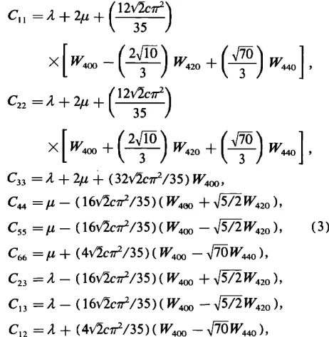
cubic crystallites, these elastic constants are not all indepen- dent. They are related to the elastic constants of single crys- tallites and texture parameters. The relations, published by Hirao et al., 8 are as follows'

C2

--,4

+ 2/t

+ (12V•crr2•

X

[W400

_(2

l•)W420

_ql_

(__•)W440

]

(,

/

[400

C33 = 2 + 2• + (32•c•/35)W4m,

C44

= • -- (16•c•/35) ( W4oo

+ •

W42o

),

C55

= • -- ( 16•c•/3 5) ( W4m

- •

W42o

),

(3)

C66

= • + (4•c•/3 5) ( W4oo

- • W4m

),

C23

-- 2 -- (16•c•/35) ( W4oo

+ •W42o ),

C•3 = A - (16•c•/35) ( W4m

- •W42o ),

C•2 = A + (4•c•/35) ( W4m

-- •W•o ),

where 2 and • are Lam• constants for the corresponding isotropic (texture-free) material and c is a measure of the elastic anisotropy of the individual crystallites. The isotropic

Lam• constants and the anisotropy constant can be obtained

from single crystal elastic constants c 0 via different averag- ing methods. Voigt, Hill, and Reuss averaging methods are

commonly used in texture study, owning to their simplicity. The Lam• constants for these averaging methods are given

in Ref. 8 as

(2 +2•)v--Cll --2Cv/5 , •V =C44 +Cv/5,

(X + 2•)• = 2(s• + s•2 - s/5)/

[ (S• + 2S•2

)(S44

+ 4S/5) ],

•R -- (S44

+ 4S/5) --1,

(x + 2•)• - [(x + 2•)• + (x + 2•)• ]/2,

(4)

•H = (•v + • )/2,

C

V :Cll --C12 -- 2C44

, C

R -- -- 4•S,

C H -- (C V +C R)/2, S--Sll --S12 --S44/2,

where

s

0 are elastic

compliances

for single

crystallites.

in an aluminum plate. References 23 and 24 include some examples of similar dispersion curve plots with wider ranges of k and • for different orthotropic materials. The phase velocities, defined as o/k, can then be calculated for differ- ent frequencies easily.

When propagating in the 0 ø and 90 ø directions, So waves

may be described as a superposition of plane longitudinal partial waves (L) and vertically polarized shear partial

1.6

•.2

0.8

0.4

0.0

0.0 0.2 0.4 0.6 0.8 •.0

bW•:

FIG. 2. Isotropic dispersion curve for the So mode in aluminum.

waves (SV) only; they are decoupled from the horizontally polarized shear partial waves (SH). On the other hand, at 45 ø angle, all L, SV, and SH partial waves are coupled togeth- er to form the So waves. Because of this, the dispersion equa- tion for the So wave propagating at the 45 ø angle is signifi- cantly more complicated, as can be seen in Eq. (2).

Although the dispersion relations given by Eqs. ( 1 ) and (2) can be used to compute ultrasonic wave speeds from given texture parameters, the inverse problem cannot be solved analytically. Therefore, the community 13-18 has de-

veloped

approximate

procedures

to obtain

texture

param-

will use the exact dispersion relations to evaluate the accura-

cy of the two dispersion

correction

methods

9,2ø

currently

known to the authors.

II. APPROXIMATE THEORIES FOR DISPERSION

CORRECTIONS

Thompson

et al. 21 and

Lee

et al. 22 applied

the theory

of

crystalline aggregates in plates with infinitesimal thickness.

Under

that assumption,

the propagating

wave

is not disper-

stants

of the plate

22 is (after dropping

higher-order

texture

and the stress related terms):

pV 2

So

( a ) -- CL + «a CL cos

^

^^

2a -- •/3C

^^

r ( 1 -- cos

4a),

(5)

where

C'œ-

Cll

-•'-

C'22

-- c123

-•'-

C2 ^

2 2C33

^ (tCl -- C• -- ItCh3

-- C•/C33 ]•

• __

(([(Cll

-[-

C22

)/2]

-- C12

-- (C13

-- C23

)2/2C33

)/2 -- C66)

To first order

in anisotropy,

the velocity

is then given

by

9

^

--cosZa--

4-• (1--cøs4a)

.

(6)

To express the velocity in terms of ODCs [using Eqs. (3) and (4) ], after certain approximations involving moving the W½oo terms in C33 in denominators to numerators by means of first-order Taylor approximation, Eq. ( 5 ) can be reduced

to

pV2(a)

- 1--• L+ 3•

X • 3+8•+8

W•

L

+ 2•

5

W44o

cos

4a

] ,

( 7

)

where L •2 + 2•, P•2, and c is an anisotropy constant also

I

defined in Eqs. (4). Similar approximation to Eq. (6) leads

to

V(a)

=

•/ ( 1

--

p2/L

2)

•

35 (Li_--p2)

v;•

3+8-•+8-•-

7

X W42o

cos

2a + 2x/-•

W44o

cos

4a .

From Eq. (7) or (8), linear combinations of velocities mea-

sured for a = 0 ø, 45 ø, and 90 ø can then be taken to obtain the

values of W4oo, W42o, and W440 .

Since no plate is infinitesimally thick, wave propagation in a plate is always dispersive. Although this effect is small for thin plates, so is the effect of texture. Thus the experimen- tal data must be corrected for dispersion if quantitative val- ues of the texture parameters are to be obtained.

The So waves used in texture studies are generally weak- ly dispersive, with a typical measurement frequency of 500 KHz and plate thickness of a few millimeters. In order to reduce the error introduced by the dispersion, Thompson et

al. 9 suggested a simple dispersion correction approach.

Starting

from the measured

phase

velocity

Vp,

the data

were

corrected to estimate the long wavelength limit of that veloc-

ity, V•im,

by assuming

the ratio Vp/Vii

m to be the same

in the

weakly anisotropic plate as it would be in an isotropic plate of the same thickness. The corrected velocities (long wave- length limits) were then used in Eq. (7) or (8). In our ex-

perimental work, 9'17'18 the dispersion correction normally

amounts to less than 10% of the measured velocities, and the

dispersion correction method described above was intuitive- ly believed to be reasonable. This correction improved the

accuracy of estimates of the ODCs, particularly on W400, as

expected. However, no rigorous evaluation of the range of

accuracy of this approach was made.

Hirao and Fukuoka 2ø have proposed another dispersion

correction method. They have developed a dispersion equa- tion for wave propagation in orthotropic plates under a per-

turbation frame that neglects the involvement of $H partial waves for wave propagation in nonsymmetry directions. The dispersion equation has a form that resembles Eq. (1) and

reduces to it when the wave propagation direction is in a

symmetry direction. To develop an explicit relation between ODCs and wave speeds in different propagation directions, they then made a Taylor series expansion at zero frequency

and included one higher-order term to approximate disper- sion effects at low frequencies. After dropping higher-order

terms in Wlmn, the equation for the square of the velocity is

=

+ (2c/p[(So +doaWoo

Vso

d- (s: d- d: A ) W4:o cos (2a)

+ s4 W44o cos ( 4a ) ]. ( 9 )

(This equation was not published in Reft 20, but is an inter- mediate step. ) After a further approximation, the final equa-

tion is

Vs,,

(a) = Vox/(

1 -- A) + (c/pVo)

[ (So

+ doA)

W4oo

+ (s2 + d2 A ) W42o cos (2a)

+ s4

W44o

cos(4a) ],

(10)

where

So

= (2V2rr2/35)

[3 + 16A(A

+tt)/(A + 2tt)2],

s2 = - (8x/5rr2/35)

(3A + 2tt)/(A + 2tt), s4 = 4rr2/xf•5,

and

do = (16V2rr2pVo2)(3A

+ 2tt)/[35A(A + 2tt) ],

d 2 -- -- 16V•5rr2pVo2/35A,

with

Vo

= •/4t•

(A + t• )/p (A + 2/• ) being

the isotropic

velocity

at kb=O and A = [A/(A + 21a)]2(kb/2)2/3 describing

the dispersion. For either of these expressions, solution for the Wlm n in terms of the velocities at 0 ø, 45 ø, and 90 ø is straightforward.

Since Eq. (9) was derived via a Taylor expansion in wave vector, it is expected to be valid (or provide good ap- proximation) for small kb. This is confirmed by comparing Eqs. (7) and (9), which reveals that they are identical for

plates

of zero

thickness.

The

approximation

made

in the

der-

TABLE I. Initial ODCs for computer simulations.

Group I Group II Group III Group IV W4oo - 0.01 0.01 - 0.005 0.005 W42o -- 0.005 -- 0.005 0.003 0.003 W44o 0.0075 0.0075 -- 0.004 -- 0.004

ever, Eqs. (7)-(10) are identical in the absence of anisotro- py (texture free) in the long wavelength limit. The effects of this further approximation will be discussed in the next sec-

tion. For the convenience of discussion later on, we shall call

the Thompson's dispersion correction method applied to Eqs. (7) and (8) and the Hirao's dispersion correction method using Eqs. (9) and (10) as Thompson's-A, Thomp- son's-B, Hirao's-A, and Hirao's-B schemes, respectively.

in summary, Thompson's schemes neglect the small de- viation of the So dispersion curves of textured plates from that of the isotropic ones and Hirao's schemes use a parabol- ic approximation to the anisotropic dispersion curves to re- place the exact ones that are not suitable for the estimation of

texture parameters.

III. EVALUATION OF DISPERSION CORRECTION SCHEMES

To evaluate the performance of the dispersion correc- tion schemes mentioned above, we calculated the So wave speeds for four selected groups of ODCs as a function of plate thickness to wavelength ratio using the exact disper- sion relations presented in Sec. I. These speeds were then used as input to the dispersion correction schemes to obtain estimates of the ODCs. The first step can be considered as a forward problem while the second step is an inverse prob-

lem. The initial values for the ODCs are listed in Table I. The values of the ODCs chosen here for the simulations are real-

istic representations of values encountered in textured plates. Groups I and II correspond to relatively strong tex- tures and groups III and IV correspond to relatively weak textures. Simulations have been run for the three commonly

used cubic materials: A1, Cu, and Fe. The densities and the

single crystal elastic constants for the three materials are given in Table II. For all the simulation runs, the Hill aver- aging method was employed because it is known to be more accurate than either the Voigt or Reuss averaging method, which, respectively, provide upper or lower bounds to the isotropic moduli. The isotropic and anisotropic elastic con- stants and Poisson ratios for the polycrystalline materials are listed in Table III for the Hill averaging method. For the purpose of this paper, we neglect any errors in the Hill ap-

TABLE II. Densities and elastic constants of materials for single crystals.

C• (GPa) C•2 (GPa) C44 (GPa) p (g/cm •)

AI 108.0 62.0 28.3 2.71

Cu 169.0 122.0 75.3 8.9

Fe 229.0 134.0 144.0 7.8

TABLE III. Isotropic and anisotropic elastic constants and Poisson ratios of polycrystalline materials using the Hill averaging method.

L=A +2• P=A T=g c

(GPa) (GPa) (GPa) (GPa) c/g

A1 112.06 59.97 26.05 -- 10.77 -- 0.41 0.3486 Cu 200.73 106.13 47.30 -- 97.68 - 2.07 0.3459 Fe 272.65 112.17 80.24 -- 132.08 -- 1.65 0.2915

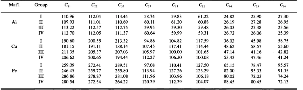
proximation. Note that the anisotropy constant to isotropic shear modulus ratio c/p in Table III for Cu or Fe is about four to five times larger than that for A1. Since the anisotropy of a polycrystal aggregate arises from the anisotropy within the single crystals and glm n are the only orientation descrip- tion parameters of the aggregate, the same set of W•,,n repre- sents different degrees of anisotropy for different materials. For the four groups of ODCs we used in our study, groups I and II for Cu and Fe exhibit the strongest anisotropy. All the rest are more weakly anisotropic, even though groups I and II for A1 have the same texture values as for the strongly anisotropic Cu and Fe cases. A feeling of the strength of the anisotropy for the four sets of ODCs in the simulation can be obtained from the elastic constants given in Table IV.

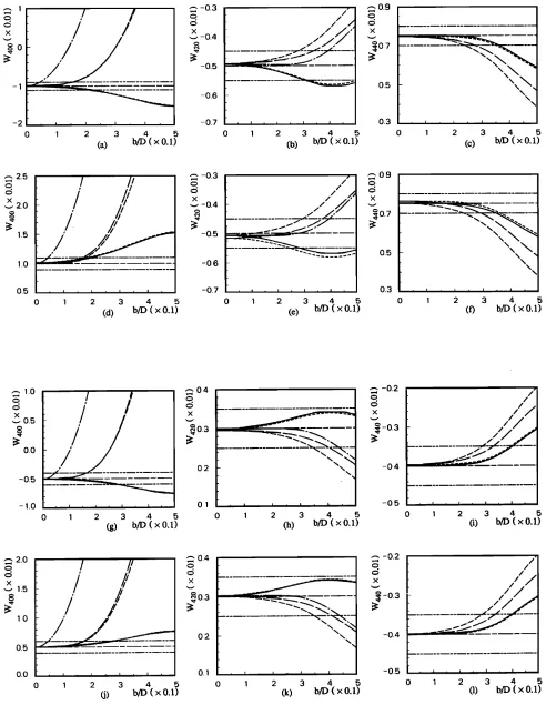
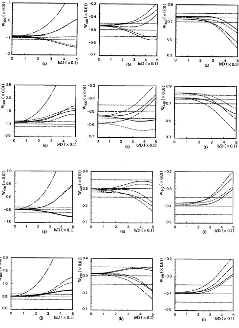
Figures 3-5 show the results from the inversion step. Here the values of the ODCs that would be predicted on the basis of different dispersion correction schemes are plotted as functions of plate thickness to wavelength ratio or b/D, where D denotes the wavelength. Please note the scales for the ordinates are different for the predictions of each of the three ODCs. For the current texture measurement configu-

ration, • 8,27 the wavelength of the So waves is about 10 mm;

the range 0-0.5 for b/D represents a plate thickness of 0-5

mm.

In addition to the four curves representing the predic- tions from Thompson's and Hirao's schemes described in the previous section, there are three horizontal straight lines in each figure, identifying the value of the ODCs assumed in the forward calculations and the target error bounds (to be discussed shortly). To see how dispersion correction

schemes influence the prediction of ODCs, the results calcu- lated directly from Eq. (7) without any dispersion correc- tions are also included in Figs. 3-5. These results are repre- sented by an extra dash-dotted curve in the W4oo and W42o figures of Figs. 3-5. In the W44o figures of Figs. 3-5, this extra curve is not plotted; it would fall on top of the curve representing the response from the Hirao's-A scheme, which uses Eq. (9). A comparison between Eqs. (7) and (9) shows that in Hirao's-A scheme, dispersion correction plays no role in the prediction of W4•o; therefore, the responses for

W•o using Eqs. (7) and (9) are identical.

Consider first the performance of the predictions of W•4o [parts (c), (f), (i), and (1) of Figs. 3-5]. For the weakly anisotropic cases [ parts (c), (f), (i), and (1) of Fig. 3, and figures (i) and (1) of Figs. 4 and 5 ], the performances of Thompson's schemes are practically equivalent, and Hir-

ao's-B scheme is found to be better than Hirao's-A scheme,

providing a wider range of reliable predictions. When the anisotropy becomes strong [ parts (c) and (f) of Figs. 4 and 5], both Thompson's-B and Hirao'soB schemes may pro- duce predictions of W4•o with relatively large errors for small thickness to wavelength ratio. This is especially true for Thompson's-B scheme, although it may sometimes give good predictions at some large thickness to wavelength ra- tio. This error is the consequence of the approximations made in going from Eq. (5) to Eq. ( 8 ) and from Eq. (9) to Eq. (10), which suggests that Eqso (8) and (10) are not favorable for such cases. Over the range of thickness to wave- length ratio plotted, Thompson's-A scheme has a longer flat region and is generally better than Hirao's-A scheme for the

TABLE IV. Elastic constants of the textured plates for the W• ... given in Table I (in GPa).

Mat'l Group C,, C• C33 C23 C•3 C•2 C44 C5• C6o

I 110.96 112.04 113.44 58.74 59.83 61.22 24.82 25.90 27.30

A1 II 109.93 111.01 110.69 60.11 61.20 60.88 26.19 27.28 26.95

III 113.22 112.57 112.75 59.95 59.30 59.48 26.03 25.38 25.56

IV 112.70 112.05 111.37 60.64 59.99 59.31 26.72 26.06 25.39

I 190.60 200.55 213.32 94.86 104.82 117.59 36.02 45.98 58.75

Cu II 181.15 191.11 188.14 107.45 117.41 114.44 48.62 58.57 55.60

III 211.35 205.37 207.03 105.97 100.00 101.65 47.14 41.16 42.82

IV 206.62 200.65 194.44 112.27 106.30 100.08 53.43 47.46 41.24

I 259.09 272.41 289.51 97.08 110.41 127.50 65.15 78.47 95.57

Fe II 246.45 259.77 255.80 113.94 127.26 123.29 82.00 95.33 91.35

III 286.86 278.87 281.08 111.96 103.96 106.18 80.02 72.03 74.24

IV 280.54 272.54 264.22 120.39 112.39 104.07 88.45 80.45 72.13

-2

•

/// ,• 0.9

-o.4 I

_l

_{. /,/}

_{I '•o• ----}

x

2_ •: 0.5

•

-06

0 1 2 3 4 5 0 1 2 3 4 5 0 1 2 3 4 5

(•)

b• ( x 0.•)

(b) b• ( x 0.•)

(c) b• ( x 0.•)

,•, 2.5

1.0

0.5

1 2 3 4 5

(d) b/D ( x o.•)

,•, -0.3

X

,• -0.4.

-0.5

-O6

-0.7

///

, I , I , I • i , I

0 1 2 3 4 5

(e) b/D

( x 0.1)

7 ... •• ' • ...

t 5

3 , i , i , i , i , i

0 1 2 3 4 5

(f) b/D ( x 0.1)

10

• 04

• -0.2

x x

0.5

•

o.o ,'

:

0 1 2 3 4 5 0 1

(g) b/D ( x 0.1)

2 3 4 5

(h) b/D ( x 0.1)

-1

o 1 2 3 4 5

(i) b/D ( x 0.1)

2.0

x

1.0

0.5

0.0

// j

, I ,

o 1

I , I • I ,

2 3 4 5

(j) b/D ( x 0.1)

•0.4

• -0.2

//

...

X

•ø0.

3

I

•-0.3

o2

-o.,

0.1 , -0.5

0 1 2 3 4 5 0 1 2 3 4 5

(k)

b• ( x o.•)

d)

b• ( x o.•)

FIG.

3.

Comparison

of

dispersion

correction

schemes

in

predicting

ODCs

for

A1.

(a)-(c)'

group

I; (d)-(f)'

group

II; (g)-(i)'

group

III; (j)-(1)'

group

IV.

--, Thompson's-A

scheme;

---,

Thompson's-B

scheme;

-- -, Hirao's-A

scheme;

-- --, Hirao's-B

scheme;

.... , no

dispersion

correction;

---, exact

value;

... , target

error

bounds.

The

target

errors

are

0.001,

0.0005,

and

0.0005

for

W4oo,

W42o,

and

W44o.

1304

-2 i I i I , I f I f

1 2 3 4 5

(a) b/D ( x 0.1)

x -0.4

-05

-06

-0.7

/ / /

2 3 4 5

(b) b/D ( x 0.1)

0.{

0.:

1

'!

I , I , I ,

2 3 4 5

(c)

b/D

( x 0.1)

•2.5

1.0

O5

-0.3

-04

-05

-O6

-O7

0 1 2 3 4 5 0 1

(d) b/D ( x 0.1)

// //

///

2 3 4 5

(½) b/D

( x 0.1)

_

.

05

03 , i , i , i , i ,

0 1 2 3 4 5

(f) b/D ( x 0.•)

-O5

- 1.0

•0.4

•- -0 2

/

ß X X

/

...

/

o

-o

•=-

•

...

0 1 2 3 4 5 0 1

(g) b/D

( x 0.1)

2 3 4 5

(h) b/D ( x 0.1)

o 1 2 3 4 5

(i) b/D ( x 0.1)

2.0

ß X

1.O

0.0 • 0.1 , I , i , I , I , 0 1 2 3 4 5 0 1 2 3 4 5

(j) b/D ( x 0.1) (k) b/D ( x 0.1)

-0.5

1 2 3 4 5

(1) b/D ( x 0.1)

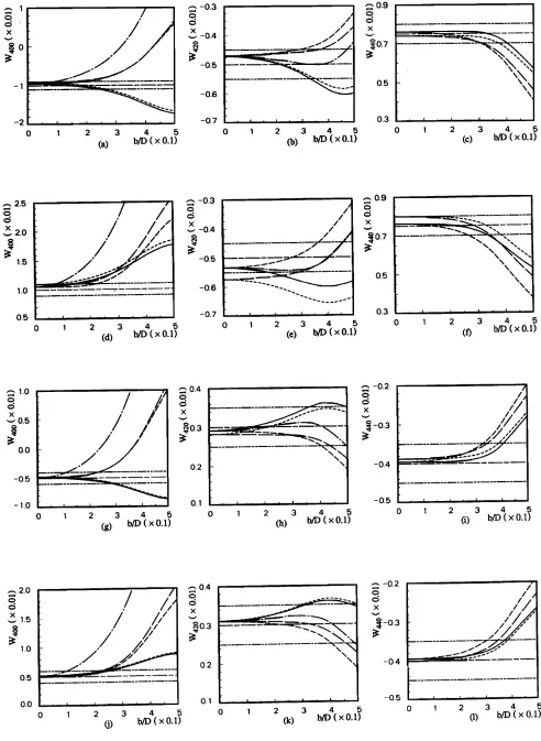
FIG.

4. Comparison

of

dispersion

correction

schemes

in predicting

ODCs

for

Cu.

(a)-(c).

group

I; (d)-(f).

group

II; (g)-(i). group

III; (j)-(1).

group

IV.

value; .... , target error bounds. The target errors are 0.001, 0.0005, and 0.0005 for W4oo, W42o, and Wgg o .

-1

-2

o 1 2 3 4 5

(a)

b/D

( x 0.1)

-0.3

-0.4

-0.5

-0.6

-0.7

[

t

, I i

1

I i i I .,.

2 3 4 5

(b) b/D

( x 0.1)

J.5

0.3

J i I i I i

0 1 2 3 4 5

(c) b/I) ( x 0.1)

•'•

/

•

_o.,,

,,

/

1.0 • -0.6

0.5 -0.7

0 • 2 3 4 • 0 • 2 3 4

(d) b• ( x 0.•)

(c) b• ( x 0.•)

i I

0 1 2 3 4 5

(0

b/D

( x 0.1)

-0.5

-1.0

/

?

./ //

/

/

i i ! i i i ,

0 1 2 3 4 5

(g) b/D

( x 0.1)

t, ,, = • -0.2 ,

... x

0.2

\x

-0.4

0.1 -0.5

0 1 2 3 4 5

(h)

b/D

( x 0.1)

0 1 2 3 4 5

(i)

b/D

( x 0.1)

.-. 2.0

x 1.5

1.0

0.5

0.0

o 1 2 3 4 5

(j)

bid ( x 0.1)

RO

3 -•--_--•••--, - •-0.3

,

02

-04 "--'-:""'"'

• ....

0 1 -0.5

0

1

2

3

4

5

0

1

2

3

4

5

(k) b/D

( x 0.1)

(t) b/D

( x 0.1)

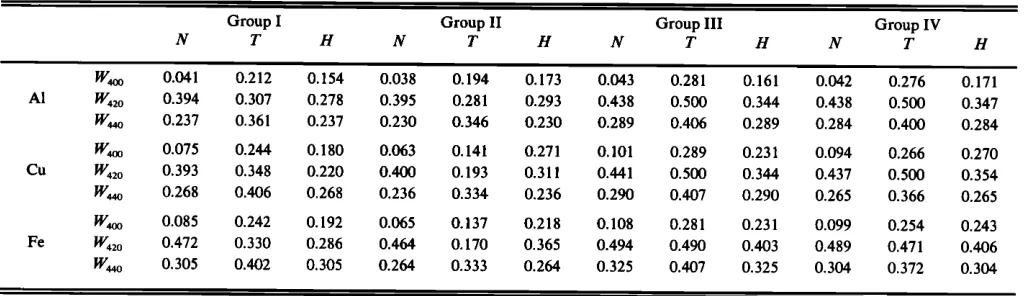
FIG.

5.

Comparison

of

dispersion

correction

schemes

in

predicting

ODCs

for

Fe.

( a

)-( c)'

group

I; ( d

)-(f)' group

II; (g)-(i)'

group

III; (j)-(1)'

group

IV.

--, Thompson's-A

scheme;

---,

Thompson's-B

scheme;

-- -, Hirao's-A

scheme;

----., Hirao's-B

scheme;

.... , no

dispersion

correction;

•- •, exact

13o6

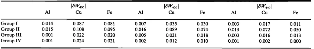
TABLE V. Acceptable limits of thickness to wavelength ratio for the error bounds: 16•V4oo [--0.001, 16W42o [, and 16•V44o I •0,ooo5 <S, no dispersion

correction; T, Thompson's-A scheme; H, Hirao's-A scheme).

Group I Group II Group III Group IV

N T H N T H N T H N T H

W4oo 0.041 0.212 0.154 0.038 0.194 0.173 0.043 0.281 0.161 0.042 0.276 0.171 A1 W42o 0.394 0.307 0.278 0.395 0.281 0.293 0.438 0.500 0.344 0.438 0.500 0.347 Wn4o 0.237 0.361 0.237 0.230 0.346 0.230 0.289 0.406 0.289 0.284 0.400 0.284 W4oo 0.075 0.244 0.180 0.063 0.141 0.271 0.101 0.289 0.231 0.094 0.266 0.270 Cu W42o 0.393 0.348 0.220 0.400 0.193 0.311 0.441 0.500 0.344 0.437 0.500 0.354 Wn4o 0.268 0.406 0.268 0.236 0.334 0.236 0.290 0.407 0.290 0.265 0.366 0.265 W4oo 0.085 0.242 0.192 0.065 0.137 0.218 0.108 0.281 0.231 0.099 0.254 0.243 Fe W42 o 0.472 0.330 0.286 0.464 0.170 0.365 0.494 0.490 0.403 0.489 0.471 0.406 Wn4o 0.305 0.402 0.305 0.264 0.333 0.264 0.325 0.407 0.325 0.304 0.372 0.304

cases studied. In fact, in the region b/D = 0-0.25, the errors associated with the prediction by Thompson's-A scheme are very small. Since in Hirao's schemes W•4o is not corrected for dispersion, when compared to Thompson's schemes, one finds that improvement can be made with the inclusion of the dispersion effect, although this effect is not as strong as that for W4oo (see the discussions on W4oo ).

Now consider the performance of the predictions of W42o. 3/s can be seen in parts (b), (e), (h), and (k) of Figs. 3-5, Thompson's and Hirao's schemes influence the predic- tion of W4,•o in opposite directions in all the cases studied, although the amount of influence is about the same in the range of b/D ---- 0-0.25. Except for the strongly anisotropic cases, Hirao's-B scheme generally gives better predictions than Thompson's schemes and Hirao's-A scheme. Similar to the predictions of W•4o, Thompson's-B and Hirao's-B schemes may give unacceptable errors to the prediction of W4,•o when the anisotropy of the plate gets strong. However, when compared to the predictions without dispersion cor- rection, one finds that neither Thompson's nor Hirao's schemes are as good as the uncorrected predictions for all the cases studied. This clearly indicates that dispersion correc- tion is really not necessary for W6,•o. As a matter of fact, the curves representing the predictions of W6:o without the dis- persion correction in general have a very flat region for

b/D ---- 0-0.25. These results are not fully understood. It can

be argued that, since W6,•o is known to be a measure of in- plane anisotropy, having little to do with the plate thickness that strongly influences the dispersion characteristics, no correction is needed. However, this same argument would apply to predictions of W•o. Since Hirao's-A scheme, corre- sponding to no correction, gives the poorest results for W64o,

further factors must be involved.

The situation is somewhat different for the prediction of W6oo, which is rather sensitive to the way in which a correc- tion is made for dispersion. A glance of parts (a), (d), (g), and (j) of Figs. 3-5 reveals that both Hirao's and Thomp- son's schemes improve the estimation of W6oo significantly. Noting the compressed scale of these plots we see that the errors are considerably greater than in the predictions of W62o and W64o. Hirao's-A and Hirao's-B schemes generally exhibit similar performance, with the former being some-

what more accurate. Thompson's schemes also exhibit simi- lar performance, particularly when the anisotropy is not strong. Depending on the sign of W6oo, Thompson's and Hirao's schemes may affect the prediction of W6oo in either the same or the opposite direction. For weakly anisotropic textured plates, Thompson's schemes generally predict W6oo with smaller errors. When the anisotropy becomes stronger, Hirao's schemes can be superior than Thompson's schemes. This fact is due to the nature of the approximations made in the Thompson's and Hirao's schemes. For Hirao's schemes, the accuracy of the prediction is closely related to the value of b/D; it is relatively insensitive to the degree of anisotropy. The performance of Thompson's schemes, on the other hand, depend on the smallness of the difference between the isotropic and anisotropic dispersion curves. For most of roll- ing and annealing textures, particularly on A1 plates, where the anisotropy is not very strong, this difference is indeed small. In this case, Thompson's schemes may be more appro- priate for b/D > O. 15. The greater sensitivity of the predic- tions of W6oo to the details of the dispersion correction oc- curs because W4oo depends on the absolute, rather than

relative values of measured velocities. 9

To see how Thompson's and Hirao's schemes correct for the dispersion quantitatively, we set up the following tar-

get error bounds for each group: 16Woo I 0.001, 16w,_o 1, and 16 W44o I • 0.0005. These error bounds are chosen from a

practical point of view, as they represent the experimentally

observed differences between ultrasonic and diffraction (x-

ray or neutron) predictions of the ODCs. 9 Table V shows

the acceptable limits of thickness to wavelength ratio for Thompson's-A and Hirao's-A schemes as well as from the uncorrected equation, if one wishes to stay within these bounds for the cases studied. It gives a guideline for the va- lidity range of the current experimental configuration and dispersion correction schemes. For most metal sheets of in- terest in texture and formability prediction, the plate thick-

ness is less than 2.5 mm. This thickness is about the limit of

the present techniques if the wavelength is around the typi- cal 10 mm value. From Table V, it is readily seen that, for the prediction of W4oo, Hirao's-A scheme is not favorable for A1 when the plate thickness to wavelength ratio is larger than 0.17. With the exception of group II in Cu and Fe, Thomp-

TABLE VI. Errors for zero thickness plates ( X0.01 ) (For Thompson's-A and Hirao's-A schemes).

A1 Cu Fe A1 Cu Fe A1 Cu Fe

Group I 0.009 0.050 0.050 0.006 0.029 0.029 0.003 0.012 0.010 Group II 0.019 0.054 0.054 0.007 0.033 0.034 0.003 0.017 0.013 Group III 0.002 0.012 0.012 0.002 0.009 0.008 0.001 0.005 0.005 Group IV 0.001 0.011 0.012 0.002 0.010 0.009 0.001 0.007 0.005

TABLE VII. Errors for zero thickness plates ( X0.01 ) (For Thompson's-B and Hirao's-B schemes).

A1 Cu Fe A1 Cu Fe A1 Cu Fe

Group I 0.014 0.087 0.08! 0.007 0.035 0.030 0.003 0.017 0.011

Group II 0.015 0.108 0.095 0.016 0.089 0.074 0.013 0.072 0.050

Group III 0.001 0.022 0.020 0.005 0.021 0.018 0.003 0.016 0.013 Group IV 0.001 0.024 0.021 0.002 0.012 0.010 0.001 0.002 0.000

son's scheme provides a wider range of valid dispersion cor- rections for W400. Both Thompson's-A and Hirao's-A scheme, however, significantly improve the prediction of W400. On the other hand, the valid ranges for both Thomp- son's-A and Hirao's-A schemes for the prediction of W420 are narrower than that from the equation without dispersion

correction. it also can be seen from Table V that the vaslu

range ofb/D for Thompson's-A scheme for the prediction of W44o is from 0 up to about 0.35-0.4. The corresponding range for Hirao's-A scheme (equivalent to no correction) is

0.23-0.3.

From Figs. 3-5, one cannot fail to see that even when the

plate thickness approaches zero, where the dispersion cor-

rections are zero for all schemes, the results from the inverse

process do not give the right answers. This is not surprising. The errors for Thompson's-A and Hirao's-A schemes are due to the approximations made when developing Eqs. (5),

(7), and (9). These errors, however, are, in general, toler- able, as they are well within the target error bounds. These errors are given in Table VI for all groups. For Thompson's- B and Hirao's-B schemes, the errors in predictions of W42o and W44o at zero thickness for Cu and Fe can be large, ex- ceeding the target error bounds. Table VII lists the errors from these two schemes. A comparison of the values in Table VI to those in Table VII clearly indicates that, with few ex- ceptions, Thompson's-A and Hirao's-A schemes are better than Thompson's-B and Hirao's-B schemes for thin plates.

IV. CONCLUSIONS

We have evaluated the two available dispersion correc-

tion methods using numerical simulations to estimate the

range of validity of each correction scheme. In general, both Thompson's-A and Hirao's-A schemes work well for plates with thickness to wavelength ratio less than 0.15. Thomp-

son's-B and Hirao's-B schemes also lead to satisfactory re- sults in this region, except for problems at small thickness to

wavelength ratios of highly textured plates of Fe and Cu. Depending on the details of texture, preference may be given to a particular scheme. For thickness to wavelength ratios larger than 0.15, each technique begins to breakdown.

Thompson's

schemes

usually

have

a greater

range

of validity

als anisotropy is strong. None of these schemes, however,

provides adequate corrections for W4oo when the ratio ex-

ceeds

0.3. Therefore,

one should

be very cautious

when

ap-

Hirao's-A

schemes

are practically

equivalent

for plates

with

a thickness to wavelength ratio less than 0.2. When this ratio exceeds 0.2, Thompson's-A scheme is recommended. In ei- ther case, the dispersion correction effects are not as domi-

nant as for W4oo. Finally, Thompson's-B and Hirao's-B

schemes

should

be avoided

when

the plate

anisotropy

is very

strong, due to the relatively large errors at the small thick-

ness to wavelength ratio.

ACKNOWLEDGMENTS

Ames

Laboratory

is operated

for the U.S. Department

W-7405-Eng-82.

This work was supported

by the Director

for Energy

Research,

Office

of Basic

Energy

Sciences.

• R.-J. Roe, J. Appl. Phys. 36, 2024 (1965). R.-J. Roe, J. Appl. Phys. 37, 2069 (1966).

G. J. Davies, D. J. Goodwill, and J. S. Kallend, Met. Trans. 3, 1627

(1972).

D. R. Allen and C. M. Sayers, Ultrasonics 22, 179 (1984).

C. M. Sayers, Ultrasonics 24, 289 (1986).

6 R. B. Thompson, S.S. Lee, and J. F. Smith, J. Acoust. Soc. Am. 80, 921

(1986).

7 A. V. Clark, Jr., R. C. Reno, R. B. Thompson, J. F. Smith, G. V. Blessing,

R. J. Fields, P. P. Delsanto, and R. B. Mignogna, Ultrasonics 26, 189

(1988).

8M. Hirao, K. Aoki, and H. Fukuoka, J. Acoust. Soc. Am. 81, 1434

(1987).

9 R. B. Thompson, J. F. Smith, S.S. Lee, and G. C. Johnson, Met. Trans. A

20, 2431 (1989).

to H.-J. Kopineck, Nondestructive Characterization of Materials, edited by

P. H611er, ¾. Hauk, G. Dobmann, C. O. Ruud, and R. E. Green (Spring- er-Verlag, Berlin, 1989), Vol. III, p. 740.

• H.-J. Kopineck, H. Often, and H. J. Bunge, in Reft 10, p. 753. •2 M. Spies and E. Schneider, in Ref. 10, p. 296.

•30. Cassier, C. Donadille, and B. Bacroix, in Ref. 10, p. 303. •4y. Li, J. F. Smith, and R. B. Thompson, in Reft 10, p. 312.

•5 D. Daniel, K. gakata, J. J. Jones, I. Makarow, and J. F. Bussiere, Nondes- tructive Monitoring of Materials Properties, edited by J. Holbrook and J.

Bussiere (Materials Research Society, Pittsburgh, PA, 1989), p. 77.

t6 M. Muragama, K. Fujisawa, H. Fukuoka, M. Hirao, and S. Yonehara, 1989 Ultrasonics Symposium Proceeding (IEEE, New York, 1989), p.

1159.

•7 E. P. Papadakis, R. B. Thompson, S. J. Wormley, K. Forourghi, D. D.

Bluhm, H. D. Skank, Review of Progress in Quantitative Nondestructive

Evaluation 10, edited by D. O. Thompson and D. E. Chimenti (Plenum, New York, 1991 ), p. 2053.

•8 A. ¾. Clark, Jr., R. B. Thompson, Y. Li, R. C. Reno, G. ¾. Blessing, D. ¾.

Mitrakovic, R. E. Schranm, and D. Matlock, Res. Nondestr. Eval. 2, 157

(1990).

t0 R. B. Thompson, Physical Acoustics XVII, edited by R. N. Thurston and

A.D. Pierce (Academic New York, 1990), p. 157.

20 M. Hirao and H. Fukuoka, J. Acoust. Soc. Am. 85, 2311 (1989).

2• R. B. Thompson, S.S. Lee and J. F. Smith, Ultrasonics 25, 133 (1987).

22 S.S. Lee, J. F. Smith, and R. B. Thompson, Proceedings of the 2nd Inter-

national Symposium on Nondestructive Characterization of Materials, edited by J. F. Bussiere (Plenum, New York, 1987), p. 155.

23 y. Li and R. B. Thompson, Review of Progress in Quantitative Nondes- tructive Evaluation, edited by D. O. Thompson and D. E. Chimenti (Ple-

num, New York, 1989), p. 189.

24 y. Li and R. B. Thompson, J. Acoust. Soc. Am. 87, 1911 (1990). 25 A. H. Nayfeh and D. E. Chimenti, Review of Progress in Quantitative

Nondestructive Evaluation 8A, edited by D. O. Thompson and D. E. Chi- menti (Plenum, New York, 1989), p. 181.

26 A. H. Nayfeh and D. E. Chimenti, J. Appl. Mech. 56, 881 (1989). 27 S. J. Wormley, R. B. Thompson, and Y. Li, Review of Progress in Quanti-

tative Nondestructive Evaluation 7B, edited by D. O. Thompson and D. E. Chimenti (Plenum, New York, 1988), p. 1639.