;
International Doctorate School in Information and Communication Technologies
DIT - University of Trento
R
EAL-T
IMEE
VENTC
ENTRICD
ATAI
NTEGRATIONMajed Ayyad December 2014
Advisor:
i
Abstract
A vital step in integrating data from multiple sources is detecting and handling duplicate records that refer to the same real-life entity. Events are spatio-temporal entities that reflect changes in real world and are received or captured from different sources (sensors, mobile phones, social network services, etc.). In many real world situations, detecting events mostly take place through multiple observations by different observers. The local view of the observer reflects only a partial knowledge with certain granularity of time and space. Observations occur at a particular place and time, however events which are inferred from observations, range over time and space. In this thesis, we address the problem of event matching, which is the task of detecting similar events in the recent past from their observations. We focus on detecting Hyperlocal events, which are an integral part of any dynamic human decision-making process and are useful for different multi-tier responding agencies such as emergency medical services, public safety and law enforcement agencies, organizations working on fusing news from different sources as well as for citizens. In an environment where continuous monitoring and processing is required, the matching task imposes different challenges. In particular, the matching task is decomposed into four separate tasks in which each requiring different computational method. The four tasks are: event-type similarity, similarity in location, similarity in time and thematic role similarity that handles participants similarity. We refer to the four tasks as local similarities. Then in addition, a global similarity measure combines the four tasks before being able to cluster and handle them in a robust near real-time system. We address the local similarity by studying thoroughly existing similarity measures and propose suitable similarity for each task. We utilize ideas from semantic web, qualitative spatial reasoning, fuzzy set and structural alignment similarities in order to define local similarity measures. Then we address the global similarity by treating the problem as a relational learning problem and use machine learning to learn the weights of each local similarity. To learn the weights, we combine the features of each pair of events into one object and use logistic regression and support vector machines to learn the weights. The learned weighted function is tested and evaluated on real dataset which is used to predict the similarity class of the new streamed event.
Keywords
Acknowledgments
I wish to express my sincerest gratitude to my thesis supervisor Prof. Fausto Giunchiglia. Every time, I was unsure about the right direction in my research course, a short discussion with him helped me to continue with a perfect reasoning and logic. Without his support, trust and positive thinking, this work wouldn’t be completed.
During these years, I spent my time working with different Palestinian municipalities and public safety organizations. I would like to thank every mayor and general director who enabled me to understand their problems closely and allow me to use their data for research purposes.
Special thanks to my friends and colleagues in Palestine, who helped me in building the first prototype of the event matcher. I am in debt to Fahed AL-Khabbas, Mohammad Isleem, Mohannad Sabaana, Tareq Dofish, Raed Zidat and many other colleagues who tested the system and gave me their feedback.
Contents
1 Introduction ...1
1.1 The Context ... 1
1.2 The Problem ... 7
1.3 The Solution ... 13
1.4 The Contribution ... 14
1.5 Structure of the Thesis ... 15
2 State of the Art ... 16
2.1 Similarity Measures ... 16
2.1.1 Taxonomy Based Similarity Models ... 17
2.1.2 Spatial Similarity Models ... 22
2.1.3 Temporal Similarity Models ... 26
2.1.4 Feature-Based Similarity Models ... 28
2.2 Learning Models ... 29
2.2.1 Logistic Regression ... 30
2.2.2 Logistic Regression Model ... 31
2.2.3 Regularization... 35
2.2.4 Batch vs. Stochastic Gradient Descent ... 36
2.2.5 Kernel Methods ... 37
2.2.6 Support Vector Machines ... 38
2.2.7 Pairwise Support Vector Machines ... 43
3 Framework for Event Similarity Measures ... 44
3.1 Event Type similarity ... 44
3.1.1 Events in WordNet ... 45
3.1.2 Analysis of similarity measures ... 47
3.1.3 Event Lattice ... 52
3.1.4 A lattice based similarity measure ... 57
3.2 Location Similarity ... 59
3.2.1 RCC8 relations ... 60
3.2.2 Reasoning using RCC8 Relations... 61
3.2.4 Building RCC Algorithm ... 66
3.2.5 Experiment and Validation of results ... 71
3.2.6 Spatial Similarity Measure ... 73
3.3 Time similarity ... 79
3.3.1 Time similarity measure ... 84
3.4 Participants similarity ... 86
3.4.1 Thematic Role similarity measure ... 89
3.4.2 Scene level similarity ... 89
3.4.3 Object level similarity ... 90
4 Algorithmic Framework for Learning Similarity Relations ... 93
4.1 Base and Aggregate Measures ... 93
4.2 Pairwise Classification Framework ... 94
4.2.1 Representation approaches for learning ... 95
4.2.2 Features Extraction ... 97
4.2.3 Gradient Descent Approach... 100
4.2.4 Kernel Method Approach ... 104
4.3 System Architecture ... 106
5 Implementation and Evaluation Setup ... 115
5.1 Evaluation measures ... 115
5.1.1 Resampling methods ... 116
5.1.2 K-Fold Cross-validation ... 118
5.1.3 Learning Curves ... 120
5.1.4 ROC Curve ... 122
5.1.5 Control Parameters ... 125
5.2 Data and Ground Truth Setup ... 127
5.2.1 Annotating Events ... 127
5.2.2 Handling Missing Data ... 130
6 Evaluation results ... 134
6.1 Evaluation of the similarity model ... 134
6.1.1 Overall Model Evaluation ... 136
6.1.2 Evaluating individual predictors ... 137
6.1.4 Evaluating model performance ... 138
6.1.5 Summary of results ... 140
6.1.6 Analysis of Results ... 141
7 Related Work ... 145
7.1 Related Work ... 145
7.2 Summary ... 149
8 Conclusions ... 150
8.1 Objectives and Achieved Results ... 150
8.2 Open Questions and Future Research Directions ... 151
List of Tables
Table 1-1 Some performance metrics in public safety organizations ... 6
Table 1-2 Different criteria for event identification ... 8
Table 2-1 The Topology distance between the eight topological relationships for two spatial regions ... 22
Table 3-1 Similarity measures for a set of pairs with subsumption relations ... 48
Table 3-2 Extent and Intent of sample of events ... 55
Table 3-3 DEFINING RCC8 RELATIONS ... 60
Table 3-4 Sample of spatial entities per type ... 70
Table 3-5. Examples of different times used in observations ... 79
Table 3-6 Temporal Linguistic Terms and their membership function ... 79
Table 3-7 Results of comparison different time functions ... 85
Table 3-8 Thematic role similarity example... 89
3-9 Example of participant properties ... 91
Table 4-1 Min-Max score of different similarity measures ... 98
4-2 Summary of selected features ... 100
4-3 An example of pairs in the training dataset ... 105
4-4 The pairwise kernel matrix with sample similarity measure ... 105
Table 5-1 Sample of Annotated events by end users ... 128
Table 6-1 Features and their Coefficients... 135
Table 6-2 Coefficients Wald Test ... 136
List of Figures
Figure 1-1 Flow of information in multi-tier agencies. First tier workers are called operators;
Second tier workers are called commanders ... 3
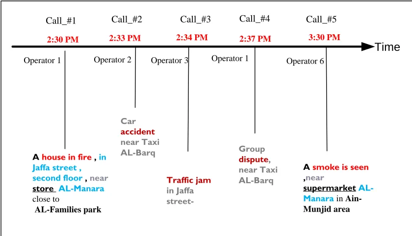
Figure 1-2 Sample of received calls in the same city showing the call number, operator who received the call and the description of the event. ... 5
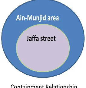
Figure 1-3 Containment relation between two regions ... 7
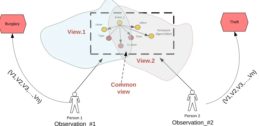
Figure 1-4 Local view of two observations ... 10
Figure 1-5 Context of two observed events ... 10
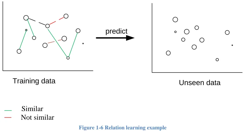
Figure 1-6 Relation learning example ... 13
Figure 2-1 Node count terminology ... 18
Figure 2-2 Conceptual neighborhood network of topological relationships -polygons ... 24
Figure 2-3 (a) direction network; (b) pattern examples; (c) ranking of similarity for the patterns in (b) ... 25
Figure 2-4 Metric distance network ... 26
Figure 2-5 Representation of two objects that each contains its own unique features and also contains common features ... 29
2-6 Logistic regression function ... 33
Figure 2-7 LINEARLY SEPARABLE CASE ... 39
Figure 2-8 – SVM Non-Linearly Separable Case ... 40
Figure 2-9 SVM mapping from input to feature space ... 42
Figure 3-1 Sample of event types occuring in a time window ... 44
Figure 3-2 Event Synsets in WordNet ... 45
Figure 3-3 Different types of human events ... 46
Figure 3-4 Example of subsumptions relations ... 48
Figure 3-5 Comparison of similarity measures for a set of pairs with subsumption relations ... 49
Figure 3-6 Example of semantic relatedness relations ... 50
Figure 3-7 Example showing overlap between concepts ... 53
Figure 3-8 Concept lattice of different events from the felony domain ... 54
Figure 3-9 Disconnected regions ... 62
Figure 3-10 Equal regions ... 63
Figure 3-11 3 Externally Connected regions ... 63
Figure 3-12 Non tangential proper part region ... 64
Figure 3-13 EC and TPP regions ... 64
Figure 3-14 Classification of a Country Region ... 66
Figure 3-15 Region Classification based on approximate area size ... 67
Figure 3-16 Approximate and exact tiles for a region ... 68
Figure 3-17 NTTP(Town, Suburb) ... 69
Figure 3-18 Map of a region created from a shape file ... 70
Figure 3-19 Visual map of different region radius coverage ... 72
Figure 3-21 City radius less than double of selected radius ... 73
Figure 3-22 topological relations neighbors graph ... 74
Figure 3-23 Metric distance network ... 76
Figure 3-24 Time linguistic terms and membership functions ... 80
Figure 3-25 Partially overlapping time intervals ... 81
Figure 3-26 Distinct time intervals ... 82
3-27 Sample pair of causal scenes containing a cross-mappings. The woman in the top scene is receiving food, while the woman in the bottom scene is giving food away [Markman and Gentner,1993] ... 88
Figure 4-1 Monadic vs. dyadic relations ... 94
4-2 Two representation of S dataset (a) feature representation (b) Kernel representation ... 96
4-3 dot-product between features vector and parameter vector ... 96
4-4 Decision boundary for a sigmoid function ... 102
4-5 Kernel similarity matrix ... 104
Figure 4-6 Event Matching Architecture ... 108
Figure 4-7 UML Event Model ... 109
4-8 Supervised Learning process... 113
Figure 5-1 Right and left data Skewness ... 117
Figure 5-2 Lambda best value ... 120
Figure 5-3 Learning curves for high bias and high variance ... 121
Figure 5-4 The confusion matrix ... 123
Figure 5-5 ROC graph with discrete classifiers ... 124
Figure 5-6 The basic interface with which our workers label each query ... 128
Figure 6-1 Coefficients using Logistic Regression Model ... 135
Figure 6-2 Receiver operating characteristic curve . Area under ROC curve =0.7984 ... 139
Figure 6-3 A test case for evaluating the similarity model ... 143
1
1
Introduction
1.1 The Context
In the broad sense, data fusion is the process of utilizing one or more data sources over time to assemble a representation of aspects of interest in an environment [Lambert, 1999]. The term is usually co-located with situation awareness which is "the perception of the elements in the environment within a volume of time and space, the comprehension of their meaning and the projection of their status in the near future" [Endsley and Garland, 2000]. Usually, data fusion problems are studied in three types of environments [Bray, 1999]:
Designed World. In which we have a relatively complete understanding of what
exists in that world and how it operates.
Real World. In which we only partially understand the physical phenomena that
are being monitored and often have very little control over it.
Hostile World. which is defined for defense applications in which some parts of
it we understand and control, but other parts are less understood and controllable.
With [Endsley and Garland, 2000] definition of situation awareness, the role of events become clear. Events reflect the changes in the real world and usually require an action to such changes. In many scenarios, reaction to events is required immediately in near real-time. However, in real world situation, detecting events mostly take place through multiple observations by different observers. For some type of events, like the meteorological events, a sequence of constrained observations, if took place in some order and locations may signal a certain type of events. This order indicates particular properties the required observations must have and how the observations must be temporally and spatially related.
How do we make sense of data fusion ?
2
making sense of probed data requires the improvement of the quality at the level of [Mitchell, 2007]:
Representation: a richer abstract and semantic meaning of individual data inputs;
certainty (a linear probability of data sets before fusion).
Accuracy: the standard deviation on data after fusion process is smaller than
standard deviation by direct source.
Completeness: bringing a complete view on the new informational situation
gained by the current knowledge in that situation.
In this thesis, we are interested to improve the quality of data that are mainly probed from human sensors and in particular who report about hyperlocal 1events such as vehicle accidents, crimes and felonies, traffic jams, floods, sit-in, gatherings and demonstrations, which are occurring at the level of a city, suburb, block, street and even at the level of a building. In this context, the efficient dissemination and processing of hyperlocal events, plays a vital role in many public and private organizations. Addressing this problem effectively has many practical applications. In particular, we envisage the following use cases:
Multi-tier responding agencies: Law enforcement, public safety and homeland
security assimilate local events in their decision-making systems to avoid a poor judgment chain from either forming or growing as well as to increase the situation awareness in their areas.
Journalists and news agencies: many organizations or individuals rely on
different sources to be instantly informed about breaking events.
Multi-national organizations: situational awareness is a core issue for some
international and multi-national organization either for security reasons for their staff or for humanitarian reasons.
Citizens: In some hot places like in Palestinian cities, recently citizens start to use
social media to increase the situation awareness before sending their children to school or traveling from one city to another.
A structured approach to a decision making process in a multi-tier agency is depicted in figure (1-2). The figure illustrates the end-to-end information flow from the site of the event until a first responder reaches that site. We can summarize the flow of information in the following main steps:
1
3
Second tier
First tier Responder
Informant event
Decision
Events pool
Ambulance
Fire /Police news
hospital
citizen
Assimilation Lodging
Figure 1-1 Flow of information in multi-tier agencies. First tier workers are called operators; Second tier workers are called commanders
Event occurrence: In real world, events erupt from a wide spectrum of sources. In the
Palestinian context, where the events in this thesis are studied, events erupt accidently and frequently. Events such as clashes, demonstrations, confrontations, strikes, sit-ins, stone throwing, shootings, road blockage, breaches impact the life of many Palestinian citizens. Consequently, these events may cause other events such as injury, property damage, fatal or death events. In addition, criminal events, traffic events, meteorological events are also among the main types of events that derive the decision making process by many citizens and organizations.
Event Detection: In this thesis, we confine our study on events that need an action to be
taken once an event has been detected. Sometimes this is called “Actionable knowledge”. Actionable knowledge has been a hot topic in data mining, where the core idea is to make sense of the mined patterns by enabling the users to utilize them in their decision making. In our context, actions have been classified as:
Response: after the event has been detected an action is needed to deal with the
4
Preventions: prediction of events based on historical analysis may require a
prevention event or a plan to deal with the potential threat, hazard or risk.
No action: With the ability to classify non-priority or non-life threading events, a
decision of not taking any action may be considered.
In most cases, citizens are the main source of information about events. The bulk of emergency events are reported through phone calls. These are life-threatening calls and usually have dedicated call lines.
Event Lodging: In order to capture as much events as possible, a dedicated team is
allocated to answer phone calls or capture event data from other sources such as RSS feeds, incident reports, street cameras, etc. Due to increasing number of events, usually this team (first tier) is not responsible of analyzing the events. Their main concern is to get as much information as possible from its source. The lodging process is standardized by using agreed vocabularies to describe the event context.
Event Assimilation: A second tier of workers is responsible for processing the lodged
events, comparing current events with recent ones, triage events to their severity level, communicate, coordinate, collaborate with other agencies based on the intelligence derived from the lodged events. This step is the fundamental currency that drives the taken decision.
Decision Making: The taken decision depends on several factors which may include the
emergency level of the incident, location of the event, available resources, dependency on other agencies, type of action needed, etc.
5
In general and in contrast to technical sensors, humans can cognitively identify and perceive complex events such as a storm or fire which are caused or constructed from different smaller events. A human can specify a relationship between different events based on their spatial, temporal and the mode of participation of different objects. Furthermore, humans can detect how an event evolves or fades through time and space. Despite of this, human capacity is limited, therefore with large volume of incoming events there is a possibility to drop some events, deploy a resource based on false alarms, deploy double resources, or causing a delay in the response time
Time
A house in fire , in Jaffa street , second floor , near
store AL-Manara close to AL-Families park Car accident near Taxi AL-Barq
A smoke is seen
,near
supermarket AL-Manara in Ain-Munjid area
2:30 PM 2:33 PM 3:30 PM
Traffic jam in Jaffa street- 2:34 PM Group dispute, near Taxi AL-Barq 2:37 PM
Call_#1 Call_#2 Call_#3 Call_#4 Call_#5
Operator 1 Operator 2 Operator 3 Operator 1 Operator 6
Figure 1-2 Sample of received calls in the same city showing the call number, operator who received the call and the description of the event.
6
allocating double resources to the same events and dispatching resources to the nearest point of the event. Furthermore, when resources are not at capacity, delays may be longer specially if the lack of resources are at the equipment and staff level. Table (1-1) list some of the metrics that are usually used to measure the performance.
Table 1-1 Some performance metrics in public safety organizations Metric Metric .
Current Value
Metric Target Value
Detect false alarms
Less than 5 %
50%
Dropped calls 10 % Less than 1 %
Avg. Target Response Time Critical Events
12-18 minutes
8 minutes or fewer
Distance from actual event location
500 meter Less than 100 meter
7
Figure 1-3 Containment relation between two regions
If information about the modus operandi is available, a thematic operators component might be used to compare the how and what facets of events . The situation in call_5 is more difficult because If none of the previous events has a terminates axiom, then call_5 might have two possibilities : a new fire event or a diminishing one.
1.2 The Problem
In this Thesis, we refer to the problem of determining whether two event descriptions (observations) refer to the same underlying entity as an event matching (linkage) problem. We define intuitively the concept matching as the task of linking a pair of events based on a joint relationship. In this context, similarity is the relationship that we would like to use as a link. Similarity indicates how much commonality and differences two stimuli (events) have. The notion of commonality and differences is used by Lin (1997) to define the similarity using an information theoretic approach based on the following three intuitions:
Intuition 1: The similarity between A and B is related to their commonality. The more
commonality they share, the more similar they are.
Intuition 2: The similarity between A and B is related to the differences between them.
The more differences they have, the less similar they are.
Intuition 3: The maximum similarity between A and B is reached when A and B are
identical, no matter how much commonality they share
8
matching has its roots in philosophy and linguistic which was discussed by [Zacks and Tversky, 2001] [Davidson, 1985] [Quine, 1985] [Davidson, 2001] [Mourelatos, 1978] under the event identification problem. As shown in Table 1. taking for example set 1, two events are similar, from a philosophic point view, if they have the same time and location. The other sets are combination of one or more elements of: time, location, physical object, cause and effect, existential conditions and properties.
Table 1-2 Different criteria for event identification Criterion Set 1 Set 2 Set
3
Set 4
Time X X
Location X
Physical object
X Cause and
effect
X Existential
conditions
X
Properties X
Cognitive scientists also studied the processes of similarity judgment. [Larkey and Markman, 2005] identified different roles for similarity which underlies fundamental cognitive capabilities. Their theory is that there are two types of differences between compared items: Alignable differences which are differences between corresponding elements of compared items. For example, an alignable difference between a car and a motorcycle is the number of wheels they have. Nonalignable differences are differences between elements that do not correspond or differences where an element in one representation does not correspond to any element in the other representation. For example, a seat belt is a nonalignable difference between a car and a motorcycle because amotorcycle has no restraining device that corresponds to a car’s seat belt. Alignable differences and nonalignable differences are psychologically distinct. Similar items tend to have more alignable differences than dissimilar items[Markman and Gentner, 1993].
The transformation model measures similarity through the use of transformational
distance [Hahn and Chater, 1998] [Goldstone, 2004]. The concept of transformational distance is defined as a function of the complexity required to transform the representation of one stimulus into the representation of another. According to
9
representation. For example, the conditional Kolmogorov complexity between the sequence 1 2 3 4 5 6 7 8 and 2 3 4 5 6 7 8 9 is small, because the simple instructions add 1 to each digit and subtract 1 from each digit suffice to transform one into the other. In other words, the similarity between two entities is the smallest number of operations that a computer program needs to transform one entity into the other.
Having reviewed different approaches from information theory, philosophy, linguistic and cognitive science, we illustrated the complexity of dealing with similarity. In order to clarify similarity assessment framework in the event context, we illustrate the assessment problem using the following example.
Motivating Example
Observer.1 and Observer.2 are looking at an occurring event. Each observer can see the
event from a different angle. Let us assume that Observer.2 is moving, while Observer.1 is not. Also let us assume that Observer.1 observed the occurrence 5 minutes after it was observed by Observer.2. The shaded area denoted by view.1 identify the boundary of the region and its environment that can be seen by Observer.1, while view.2 identify the boundary of the region and its environment that can be seen by Observer.2. Both observers are describing the event based on their angle of observation, therefore they are reasoning about the event using what is called by [C. Ghidini and F. Giunchiglia, 2001] [Giunchiglia, 1993] reasoning with viewpoints, and reasoning about belief. The first observer believes that it is a theft, while the second believes that it is a burglary. Although both observers are using the local environment to describe the event
10 Event_1 Time Type location cause effect Participant {Agent;Objct} {V 1,V 2,V 3,… ,V
n} {V1,V
2,V 3,… ,Vn} Observation_#1 Observation_#2 Theft Burglary
Person 1 Person 2
View.1
View.2
Common view
Figure 1-4 Local view of two observations
The log of the phone calls is encoded similar to the following excerpt:
Observation.1 Observation.2
<Type > Burglary
<Location: slot1> Ramallah
<Location: slot2> In city center
<Location: slot3> near supermarket Baghdad
<Date> 12-12-2013
<Time> around 8:30 in the morning
<Agent> {{person1:attrib1,attrib2,…}, {person2:attrib1,attrib2,…} }
<Recipient:slot1> a car
<Recipient:slot2> {old man:hasage; }
<related-to> event-4
<Type > Theft
<Location: slot1> Ramallah
<Location: slot2> In Tokyo street
<Location: slot3> Not far from AL-Manara square
<Date> 12-12-2013
<Time> in the early morning
<Agent> {person1,person2}
<Recipient:slot1> a white car
<Recipient:slot2> {attrib1,attrib2,… }
<related-to>
Figure 1-5 Context of two observed events
11
As illustrated in this example, finding similarity between different observation depends heavily on the context of the observation. We define an event and its context as follow:
Definition 2.1. (Event). An occurrence (behavioral activity or natural phenomenon) happening at a specific time and location. An event entity is a tuple that takes the form:
, type, time, Loc, Ctx> (1) Where:
- , the unique identifier of an event
- type, The type of the occurrence reflects the final type after the analysis of multiple observations.
- time, the temporal part of the event. The time of occurrence can be either an
instant or a time period. A time period can be with known or unknown ends.
- Loc, the spatial part of an event. The location of an event can be either a physical
or virtual location.
- Cxt, the event context. Is a set of observations related to a single event.
Definition 2.2 (Context). Is the meta-information taken from the local knowledge of the observer which is related to the detected event, and is represented as a tuple of the form:
Cxt = (1)
O = <ID, observation-data, confidence)
O = <Obs_time, obs_loc, obs_type, participant, instrument, recipient, cause, effect, confidence>
- -Id,
- Observation-data is:
o Obs_time, The time the occurrence observed. Time can be either an instant or a time period. A time period can be with known or unknown
boundaries.
o obs_loc, The location of the occurrence from the perspective of the observer.
o obs_type, The type of the occurrence from the perspective of the observer
o Participant, Participant can have different roles such as agents or recipients.
12
o Cause, A set of events that might be the reason for this occurrence to happen.
o Effect, A set of events that be resulted from this occurrence.
- Confidence, the level of confidence the observer has in describing the occurrence. Despite the availability of different models for comparing two objects or entities, selecting one model cannot handle the complexity of comparing a pair of events. Events are complex entities that require employing a similarity framework which can handle:
Semantic similarity among event-types. Spatial similarity among event-locations Temporal similarity among event-times
Feature-based or alignment based similarity among event-participants.
Existing algorithms only handle separately each component. Furthermore, measuring semantic similarity between event types only return a value indicating the degree of similarity between a pair objects. They do not indicate why two objects are similar or not similar. Exploiting the context which includes location, time, environmental conditions, participants, activity, nearby objects, instruments, and nearby people, explains why two events are assigned a particular similarity score and help in detecting errors in the automated similarity measures as well as strengthen our understanding on what factors contribute to similarity between events.
Problem Definition
Consider an observation stream as a time ordered series of observation records
and a stream of events
,
where has the form{
Consider a delta-based time sliding window model W = { , where
is the latest time slot and is the first time slot in the window and the first to
be evicted when the time shifts by b to the new slot .
Hence the event matching -problem is to group the events arriving in the last b time periods of the stream S into a set of clusters such that each cluster
13
1.3 The Solution
We consider the problem of determining whether a pair of events, belong to the same class or not, as a pairwise binary classification problem. The main objective of pairwise classification is to infer the similarity relation between two events. We have two classes: similar and not similar. To learn the similarity relation between a pair of events, we trained a classification function g from a set of training examples where for each pair
of the example, we know if the pair belongs to the same class ( ) or not ( .
As shown in figure 1-6, given a dataset of similar pairs and non-similar pairs of events and a feature representation that characterize these relations. We can infer a model that if given a new pair of events, can predict the relation between them.
Similar Not similar
predict
Unseen data Training data
Figure 1-6 Relation learning example We decompose the matching task into three sub-tasks:
1. Feature selection: we use the similarity measures as the features of similar or
non similar events.
2. Learning task: from the training set, we learned a metric so the prediction model
14
phase is a similarity matrix which is used to assign the new event to a new or existing cluster.
3. Validation: we validate the model using real-data set .
For metric learning, we consider the two events as two records and follow the procedure of record linkage problem. The theory and techniques of record linkage date back to pioneering work by Fellegi and Sunter [Fellegi and Sunter, 1969] in their seminal paper “A Theory for Record Linkage”. In relational management database system, a record linkage problem is addressed by applying different similarity algorithms [Elmagarmid et al., 2007] [Banu, 2012] at three different levels:
Record level Field level Index level
We also show the system architecture used to automatically compare events on a stream and identifies past events similar to newly detected ones. The events we monitor are local in contrast to global events, that is, they happen at a specific region in a given time period.
1.4 The Contribution
In this thesis, we provide the following contributions:
The main contribution of this thesis is represented in chapter 3 and chapter 4. Mainly the work on identifying suitable and adequate similarity measures for each element of the observed event. In essence, this thesis includes the following important contributions:
Provides adequate type, spatial, temporal and thematic role similarity functions. The design of these similarity functions considers similarity knowledge combined from cognitive point of a view as well as functional point of view. Similarity measures in addition to semantic similarity and relatedness considers:
• Location relations (topology, orientation and direction) • Temporal relations (linguistic terms and fuzzy intervals) • Causes and effects
• Agent • Patient • Functions
15
A quantitative analysis of different similarity measures and their limitations to be used in finding similar events. We analyzed the adequacy of existing similarity measure for the task of learning the weights of event types . For other aspects or facets of the event, we discussed the concept of similarity from numerous view-points and their computational approach, in particular, the alignmenet model, transformational model and relational model, of similarity.
A computation framework to calculate similarity is presented using supervised learning approaches. Mainly similarity between pairs of events are learned using logistic regression and support vector machines.
We also evaluate our approach and show that the approach is applicable to real-life scenarios and applications.
1.5 Structure of the Thesis
The thesis is organized as follows.
Chapter 2 introduces the state of the art covering the topics of similarity measures and learned metrics.
Chapter 3 is divided into four main sections covering: type-similarity; location similarity ; time similarity and thematic role similarity.
Chapter 4 provides a computational framework to learn similarity weights and describes the architecture of the system for event matching.
Chapter 5 describes the evaluation measures to assess and select the model as well as methods of collecting and validating the data used in our experiments.
Chapter 6 shows the results of our experiments.
Chapter 7 provides a review of related work
16
2
State of the Art
In the previous chapter, we explored the main theories and broad definition of similarity between two stimuli or objects. In this chapter, we will introduce the approaches and techniques to measure and learn the similarity. In section (2.1), the notion of similarity, its definition and different related similarity measures will be introduced focusing on the following dimensions: concept similarity, spatial similarity, temporal similarity and attributal similarity. In particular, this will cover the four main dimensions of any event. In the second section, we will introduce the learning theory and two algorithmic approaches used to learn a model. In particular, we will introduce logistic regression and support vector machine.
2.1 Similarity Measures
As argued by [Goodman, 1972] [Medin et al., 1993] there is no global agreement on how similarity is measured or defined. Goodman argues that the similarity of A to B is an ill-defined unless one can say in what respects. To define a frame of reference to the task of finding similar events, we argue that two events are similar based on the similarity between their types, spatial, temporal and participants aspects. Since we are comparing a pair of events using their contexts then we confine our literature review to the similarity measures that are related to the context elements:
o Time, The time the occurrence observed. Time can be either an instant or a time period. A time period can be with known or unknown boundaries.
o Location, The location of the occurrence from the perspective of the observer.
o Type, The type of the occurrence from the perspective of the observer
o Participant, Participant can have different roles such as agents or recipients.
A similarity measure is a function which computes the degree of similarity between pair of objects. Although there is no universal agreement as to a definition of similarity, its range manifestations map to the range [-1,1] or [0,1].
Definition 2.1[Balcan, 2008] A similarity function over X is any pairwise function
17
Besides the formalism introduced in Definition 2.1, other mathematical ways to represent similarity can be defined using distance notation and ranking [ Richter,1992] . A ranking similarity is relative similarity between two pairs.
Ranking. For two pairs x,y and z,w, SIM(x,y,z,w) means that y is at least as similar to x
as z is to w. This is equivalent to
Distance. A function d(x, y): X × X→ R+ measuring the distance between x and y.
A function , is commonly called a distance measure if it satisfies the following properties:
Non-negativity:
• Identity of indiscernibles:
• Symmetry:
• Subadditivity (triangle inequality):
2.1.1 Taxonomy Based Similarity Models
Many similarity measures have been proposed based on the availability of comprehensive taxonomies, ontologies or lexical databases such as [WordNet, 2010] or the Gene Ontology [GO, 2000] in bioinformatics. A vast amount of existing similarity measures use WordNet as the basis to compute similarity between concepts. Measuring the similarity or distance between concepts is based on measuring the semantic similarity or semantic relatedness between two concept words or phrases. The difference between semantic similarity and semantic relatedness is explained by is [Resnik, 1995] as “Semantic similarity represents a special case of semantic relatedness: for example, cars and gasoline would seem to be more closely related than, say, cars and bicycles, but the latter pair are certainly more similar”.
18
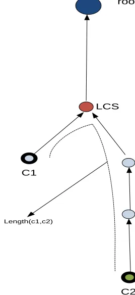
Dist ( ): The length of the shortest path from synset to synset .
LCS ( ): The lowest common subsumer of . The Least Common
Subsumer of two concepts A and B is "the most specific concept which is an ancestor of both A and B", where the concept tree is defined by the is-a relation
Depth( ): the length of the path to synset ( from the global root entity, and
depth(root)=1.
deep_max: the max depth(ci) of the taxonomy
hypo(c): the number of hyponyms for a given concept c.
node_max: the maximum number of concepts that exist in the taxonomy.
root
LCS
C1
C2 Length(c1,c2)
Figure 2-1 Node count terminology
Wu and Palmer’s Similarity Measure. [Wu and Palmer,1994]
The similarity between a pair of concepts is calculated using the formula:
19
Where
N3 is the number of nodes from the most least common subsumer (LCS) of and to the root.
N1 is the number of nodes on the path from to the node of least common subsumer (LCS)
N2 is the number of nodes on the path from to the node of the least common subsumer (LCS)
The score in wup is 0 < score <= 1.
When two concepts are the same, the score is one
Wup depends on the depth of the nodes
Leacock and Chodorow’s Similarity Measure [Leacock and Chodorow, 1998]
Where, is the shortest path between the synsets and D the total depth of the of the taxonomy. The measure us node-counting for finding the
PATH Similarity Measure [Rada et al.,1989]
This module computes the semantic relatedness of word senses by counting the number of nodes along the shortest path between the senses in the 'is-a' hierarchies of a taxonomy.
The measure also uses node-counting scheme
Resnik Similarity Measure [Resnik, 1995]
Resnik showed that semantic similarity depends on the amount of information that two concepts have in common, this shared information is given by most least common subsumer (LCS) that subsumes both concepts. If LCS does not exist then the two concepts are maximally dissimilar.
Resnik semantic similarity is defined as:
20
Where, the information content can be quantified as the negative of the log likelihood,
the probabilities of concepts in the taxonomy is estimated using the formula:
Where, where W(c) is the set of words (nouns) in the corpus whose senses are subsumed by concept c, and N is the total number of word (noun) tokens in the corpus that are also
present in WordNet. A snippet from information content file
[http://ws4j.googlecode.com/svn-history/r3/trunk/edu.cmu.lti.ws4j/src/main/resources/ic-semcor.dat]
wnver::eOS9lXC6GvMWznF1wkZofDdtbBU 1740n 128767 ROOT
1930n 69661 2137n 59062 2452n 3669 2684n 39997 3553n 32734 3993n 0 4258n 20896 4475n 20800 5787n 0 5930n 0 6024n 0 6150n 0 6269n 8 6400n 0 6484n 87 7347n 19753 7846n 19196 15388n 1124
the probabilities of concepts in the taxonomy were estimated from noun frequencies gathered from the one-million-word Brown Corpus of American English. Frequency counts are based on the number of senses a word has. Because Resnik measure is using as a corpus to calculate the information content, it is sometimes classified under the corpus based similarity models.
21
Jiang and Conrath’s measures semantic distance between two concepts taking into consideration both the information content and edge-counting. Therefore, sometimes this method is classified under hybrid methods that combines both: information content and edge-counting. The distance is calculated by the following formula :
Therefore the similarity is
Lin’s Similarity Measure [Lin, 1998]
Lin similarity measure is based on the following three intuitions as a basis to his model : 1. The similarity between arbitrary objects A and B is related to their commonality;
the more commonality they share, the more similar they are.
2. The similarity between A and B is related to the differences between them; the more differences they have, the less similar they are.
3. The maximum similarity between A and B is reached when A and B are identical, no matter how much commonality they share.
Lesk Similarity Measure [lesk, 1985]
Lesk proposed that the relatedness of two words is proportional to to the extent of overlaps of their dictionary definitions. The adapted leask [Banerjee and Pedersen, 2002] LESK measure is based on adapted uses WordNet as the dictionary for the word definitions. A combination score
22 2.1.2 Spatial Similarity Models
There are substantial work on similarity between geo-concepts [Schwering and Raubal, 2005 ] [Shariff et al., 1998] [Rodríguez and Egenhofer, 2003] [Rodríguez et al., 1999] [Rodríguez and Egenhofer, 2004]. Shariff et al. developed a model defining the geometry of spatial natural-language relations following the premise topology matters, metric refines [Shariff et al., 1998]. [Schwering and Raubal, 2005] show that people's choice of spatial relations to describe two objects differs depending on the meaning of objects, their function, shape and scale. The matching-distance measure [Rodríguez and Egenhofer, 2004] computes similarity between geo-concepts by combining different weighted similarity functions from the sub-classes of the main concept which are part, functions and attributes. The distance-matching measure is based on the comparison of distinguishing features and uses the shortest path for determining the distinguishing features in an entity class’s definition.
While measuring similarity between geo-concepts is an important aspect, we need to focus on this thesis on measuring the proximity of two places or locations rather than computing similarity between their classes. Therefore in the rest of this section, we will focus on reviewing related literature that measures similarity between locations based on their topological, orientation and directional relations.
[Freksa, 1992b] created the conceptual neighborhood network based on Allen’s 1-D interval relations. The conceptual neighborhood approach is based on the transformation model, in which similarity is measured according to the distance between two concepts in a network. Using the conceptual neighborhood, [Egenhofer and Al-Taha, 1992] worked on spatial relation similarity for the topological relations. They derived gradual changes of the topological relationship based on Egenhofer’s 9-intersection model. They created a conceptual neighborhood of the topological relationship and calculated the distance as table 2-1 illustrates.
Table 2-1 The Topology distance between the eight topological relationships for two spatial regions Disjoint Meet Equal Inside coverdBy Contains Covers overlap
Disjoint 0 1 6 4 5 4 5 4
Meet 1 0 5 5 4 5 4 3
Equal 6 5 0 4 3 4 3 6
Inside 4 5 4 0 1 6 7 4
coverBy 5 4 3 1 0 7 6 3
Contains 4 5 4 6 7 0 1 4
covers 5 4 3 7 6 1 0 3
23
[Papadias and Dellis, 1997] extended this model into a higher dimensional space to address spatial relationship similarity on topology, direction and metric distance. For higher dimensions they consider a relation set r which represents a disjunction of relations. The distance between a relation set r and a primitive relation R is the minimum distance between any relation of the relation set and R:
Topology-Direction-Distance (TDD) [Li and Fonseca,2006 ]
The TDD spatial similarity model utilizes a similarity measure that integrates four similarity models which are the geometric model, the feature contrast model, the transformation model, and the structure alignment model. The TDD model builds on the Conceptual Neighborhood Approach [Freksa, 1992] [Egenhofer and Al-Taha,1992]. The level of comparison is taken at two levels :
1. Scene level : for a scene the spatial or non-spatial relationship is measured. The spatial relationships are measured using the following relations: topological, directional, metric distance and distribution. The non-spatial relationship is measured using attribute distance.
2. object level : for objects the attributes of the objects in the scene are measured. Object attributes are measures using types of objects and attribute comparison.
The final similarity is a weighted measure
24
by default the model gives different weights for each parameter
The Topological Relationship
The computational framework is based on the transformation cost, but unlike the traditional transformation which assumes that transformation across all edges is the same, the TDD considers two types of transformation: inter-group and intra- group. If two nodes belong to different groups, the transformation cost is called inter-group cost; otherwise, the transformation cost is called intra- group cost. Directed by this principle, in Figure (2-2), adapted from [Li and Fonseca, 2006], the inter- group cost is set as 3, while the intragroup cost is set as 2 with an exception of transforming from contain to contain&meet. Nodes of contain and contain&meet can be considered as a sub-group within the group of overlap in different levels, hence the transformation cost is set as 1 which is one degree less than the intra- group cost.
y x
x y
x
y
y x
y x
x y
y x
y x 3
3
3 3
1 1
3
2
2 2
disjoin
meet
overlap
contain
Contain & meet
equal
25
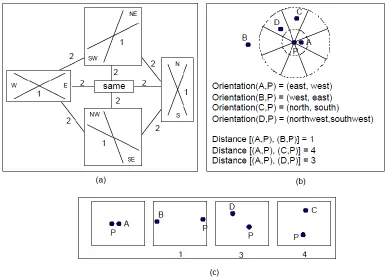
Directional Relationship
In the TDD model,using the transformation cost from one node to another in the p/2 directional network as shown in figure 2-3, which constitutes of 5 nodes {east, west}, {northeast, southwest}, {north, south}, {northwest, southeast}, and {same}. The cost of the transformation from one node to its neighbor is 2. The cost for switching the direction inside a node is 1 as.
Figure 2-3 (a) direction network; (b) pattern examples; (c) ranking of similarity for the patterns in (b)
Distance calculation
Using a metric distance network of four nodes ({equal, near, medium, far}) as shown figure 2-4, the transformation cost is set as 1. If in one scene, the metric distance
26
far
meduim
near
equal
Figure 2-4 Metric distance network
2.1.3 Temporal Similarity Models
In this section we introduce a special type of similarity measures to compare two time intervals of fuzzy characteristics. It is very common that users or observers describe the time of an event using a fuzzy temporal term such as “in the early morning” and “ around 8:30”. In the literature there is a substantial work on comparing fuzzy objects, based on fuzzy-set-theoretical concepts.
We confine our review here to methods using generalized fuzzy numbers, which is a common approach to represent time intervals and time instants. A generalized fuzzy number , where and , is a fuzzy subset of the real line R with membership function which has the following properties[chen and chen, 2003] :
1. is a continuous mapping from R to the closed interval [0,w] 2. for all
3. is strictly increasing on [a,b]
4. w for all , where w is a constant and 5. is strictly decreasing on [c,d]
6. for all
In a generalized fuzzy number, if is linear in [a,b] and [c,d] then it is called a generalized trapezoidal fuzzy number.
27
For any 2 trapezoidal fuzzy numbers and , there exists different approaches to find similarity between fuzzy numbers .
Chen similarity measure [Chen, 1996]
Hsieh and Chen similarity measure [Hsieh and Chen, 1999]
where,
and
;
Simple center of gravity method (SCGM) [Chen and Chen, 2003]
Where,
28
2.1.4 Feature-Based Similarity Models
The feature model is based on a set-theoretic representational model . As shown in figure (2-5), A-B and B-A are the set of unique features for each object, where is the set of common features shared between the two objects. Similarity measures of feature models underlie the assumption that similarity of concepts increases the more common and the less distinct features these concepts have. The most prominent representatives of the feature-matching model is Tversky's contrast and ratio model [Tversky, 1977] .
Tversky's “Contrast Model” assumes that the similarity of object a to object b is a function of the features common to a and b ( "A and B"), those in a but not in b (symbolized "A-B") and those in b but not in a (" B-A"). In this model we have three components as illustrated in Figure (5-2) : common features of A and B, distinct features of A not in B, distinct features of B and not in.
A similarity measure based Tversky's model is given as
S(a,b) = xf(a and b) – yf(a-b) – zf(b-a).
29 + + + + + + + + + + + + + + + + + + + + + + + + + + + + + + + + + + + ++ + + + + + + o o
o oo o oooo oo
o oo o oooo
o o o oo
oo o oo
oo o oo
oo o oo
oo o oo ~ ~~ ~ ~ ~~ ~ ~~ ~ ~ ~ ~~ ~
1) Features of A only
2) o oooo Features of B only
2) ~~~~ Features common between A and B
+ + +
A -B B-A
Figure 2-5 Representation of two objects that each contains its own unique features and also contains common features
Tversky also proposed the ratio model as another matching function based on the combination of . The Ratio model is defined as follows:
Similar to this approach, the Matching-Distance Similarity Measure (MDSM) was proposed by [Rodríquez and Egenhofer, 2004] which was developed for similarity measurement of geospatial terms. This category of models was based on the ratio model that extends the original feature model by introducing different types of features and applying them to terms. There are also other similarity functions based on set theoretic measures such as Jaccard coefficient, Overlap coefficient, and Dice coefficient.
30
The General Setting for Statistical Learning Problems from examples comprises three components [Vapnik, 1999] :
1. A generator of random vectors, drawn independently from a fixed but unknown distribution P(x) ;
2. A supervisor that returns an output vector for every input vector, according to a conditional distribution function1P(y|x), also fixed but unknown;
1. A learning machine capable of implementing a set of functions .
The problem of learning is that of choosing from the given set of functions
, the one which predicts the supervisor’s response in the best possible way. The selection is based on a training set of random independent identically distributed (i.i.d.) observations drawn according to
For our task, our approach is to learn a model from examples of event pairs which are labeled similar (+1), and ones that are labeled dissimilar (-1) . The objectives in learning similarity are:
To develop a similarity classifier, that is, when given a novel pair of events, as accurately as possible, predicts the label of similarity {-1,1} for this pair.
To provide a framework for similarity search form past events, without the need to apply similarity classifier to every possible pair of events.
The function chosen by the learning machine is denoted by where is a parameter vector that should be learned to fit the data.
Since we consider the problem of determining whether a pair of events, belong to the same class or not, as a pairwise binary classification problem. In the following sections we will introduce two approaches that are commonly used to in classification problems.
2.2.1 Logistic Regression
31
model that can be used when the target variable is a categorical variable. The technique aims at modeling the relationship between a set of independent variables and the probability that a case is a member of one of the categories of the dependent variables. There are two types of logistic regression: Binary logistic regression which is used for two groups and Multinomial Logistic Regression that can be used with more than two groups. In this thesis we consider only binary logistic regression.
Logistic regression has many uses [Garson, 2009] It is used to predict a dependent variable on the basis of continuous and/or categorical independents; to determine the percentage of variance in the dependent variable explained by the independents; to rank the relative importance of independents; to assess interaction effects; and to understand the impact of covariate control variable.
1. A logistic regression model is used when the outcome variable is dichotomous. 2. Logistic regression uses binomial distribution.
3. Logistic regression does not assume a linear relationship between the dependents and the independents
4. The dependent variable in the logistic regression analysis need not be normally distributed (but does assume its distribution is within the Poisson, binomial or gamma).
5. Logistic regression coefficients estimate the odds ratio for each of the independent variables used in the model
6. The models predicts the probability within a population of an individual becoming or not becoming a case
7. Tabachnick and Fidell (2001) indicate that logistic regression is a good model when using different types of predictor variables. In this case, continuous and categorical variables were used in building a predictive model.
2.2.2 Logistic Regression Model
The basic assumption with logistic regression (binary output) is that if we have an experiment with X;y, where X the dataset of experiments and y is the binary outcomes. For each experiment the outcome is either or 1 or . We want to model the conditional probability Pr(Y = 1|X = x) as a function of x; any unknown parameters in the function are to be estimated by maximum likelihood.
Since the response variable ( ) for logistic regression is always binary (assuming only two values), its distribution is binomial.
32
is the numbers of Bernouli trials and is the probability of being in the success group
, and is the probability of being in the group . The binomial distribution has distribution function
taking natural log on the equation above and let
then the unkonwn probability is equal to
Let the variable given by
33
0 0.5
1
0
-8 -6 -4 -2 2 4 6 8
F( ) 0.5
2-6 Logistic regression function
As shown in figure 2-6, the logistic regression function takes as an input, any value from negative infinity to positive infinity, whereas the output is confined to values between 0 and 1. The variable is a measure of the contribution of all the risk factors used in the model, while represents the probability of a particular outcome, given that set of risk factors.
The central mathematical concept that underlies logistic regression is the logit—the natural logarithm of an odds ratio. The logit is the natural logarithm (ln) of odds of Y, and odds are ratios of probabilities ( ) of Y happening. Logistic regression applies the logit transformation to the dependent variable. In essence, the logistic model predicts the logit of Y from X [Peng et al., 2002b].
Odds of an event are the ratio of the probability that an event will occur to the probability that it will not occur. If the probability of an event occurring is , the probability of the event not occurring is (1- ). Then the corresponding odds is a value given by
With logistic regression the mean of the response variable in terms of an explanatory variable x is modeled relating and x through the equation .
34
and 1. The solution for this problem is to transform the odds using the natural logarithm [ Lee and Ingersoll, 2002]. With logistic regression we model the natural log odds as a linear function of the explanatory variable
and recall that
then
This indicates that the independent observations variables are linearly related to the logit of the dependent. (Menard, 2001).
Under the logistic regression model, the parameters and are estimated by the method of maximum likelihood of observing the sample values [Menard, 2001]. Maximum likelihood will provide values of and which maximize the probability of obtaining the data set. Assuming the likelihood of the parameters is given by
Since it is easier to work with the log likelihood
35
We can learn the weights either by using gradient descent or Newton’s Method
2.2.3 Regularization
It is well-known that regularization is required to avoid over-fitting, especially when there is a only small number of training examples, or when there are a large number of parameters to be learned and the degree of over-fitting depends on several factors [Ng,2005].:
• Number of training examples—more are better
• Dimensionality of the data—lower dimensionality is better • Design of the learning algorithm—regularization is better
There are three types of regularizations: L0, L1 and L2 [Hastie et al.,2001] [Ng,2005]. L1 regularized logistic regression requires a sample size that grows logarithmically in the number of irrelevant features and L2 regularized logistic regression, under rotationally invariant algorithms, required a sample size that grows linearly in the number of irrelevant features.
L0 norm (sum of non zero entries
L1 norm (sum of non zero entries ; L1 norm drives many parameters to zero
L2 norm (sum of non zero entries ;L2 norm does not achieve the level of sparseness as L1
36
which have no effect on the actual output and the subset selection which is a discrete process; its regressors are either retained or totally excluded from the model.
2.2.4 Batch vs. Stochastic Gradient Descent
Logistic regression (LR) learns weights so as to maximize the likelihood of the data .
In this thesis we will use gradient descent to learn the weights. Gradient descent is divided into two categories: stochastic (also called on–line) and batch (also called off– line) learning. Stochastic is chosen either because of the very large data set(or may be redundant) training set. On the other hand Batch training is fast for small training set. The following procedure illustrated the difference between the two methods .
Batchmode Gradient Descent
until [number of iterations or other criteria]
1. Compute the gradient
37 Stochastic mode Gradient Descent
Dountil [chosen stop criteria]
For each training example 1. Compute the gradient
2. End
2.2.5 Kernel Methods
Another approach to data classification is to treat the given data as inner products in some Hilbert space. Support vector machine (SVM), which is based on Vapnik’s statistical learning theory [Vapnik, 1999] utilizes kernel methods, and maximum margin classifiers for classification-based learning. In the following sub-sections, we provide a summary of these concepts and how they could be applied to learn the similarity between a pair of events. Like logistic regression, it requires a set of training examples with each marked as belonging to one of the categories. What makes SVMs different and more efficient is the use of kernel trick which maps the inputs into higher-dimensional feature.
The basic idea in kernel methods [Hofmann et al.,2008] is to map data from the input space into a high dimensional space (some Hilbert space ) by means of a feature map. Since the feature map is normally chosen to be nonlinear, a linear model in the feature space corresponds to a nonlinear rule in the original domain.
Most data analysis methods outside kernel methods use feature mapping to do a prediction. For each x in the set of objects concerned by the learning problem each object is represented by a set of features , with a high dimensional feature space. however, in kernel methods instead of mapping , a real valued comparison function is used which is equivalent to representing the data set of objects by similarity matrix of pairwise comparisons. The kernel function k is defined as follows:
Definition 2.1 A function is called a positive definite kernel iff it is
38
For any N >0 and any choice of real numbers
A kernel function can be seen as the dot product of the feature representation of two objects
for any
Examples of kernel functions:
Linear kernel (identity kernel) :
Polynomial kernel with degree d:
Radial basis kernel with width σ:
Sigmoid kernel with parameter a and r:
2.2.6 Support Vector Machines
Since we need to solve a binary classification problem, in the coming section we will focus only presenting SVM mathematical foundation for the binary classification case. Our goal is to solve a binary classification problem by using a linear model in the Hilbert space. The linear model is represented by the following formula:
Where and b are the parameters, is the feature representation set of N objects
and y(x) is the output of the prediction that depends on the sign of y(x), where
2.2.6.1 Binary Linearly Separable Case
In the linearly separable case, there exists one or more hyperplanes that may separate the two classes represented by the training data with high ccuracy. As show in Figure (2-7):
39
the gap or margin separating the positive and negative examples in the training data. The optimal hyperplane is then the one that evenly splits the margin between the two classes.
wx+b =1 wx+b =0 wx+b =-1 M
a) More than one solution. Different hyperplanes could classify the data
b) The hyperplane that maximizes the margin between the two classes
Figure 2-7 LINEARLY SEPARABLE CASE
(b), the data points that are closest to the separating hyperplane