www.geosci-instrum-method-data-syst.net/6/209/2017/ doi:10.5194/gi-6-209-2017
© Author(s) 2017. CC Attribution 3.0 License.
Method for processing XCP data with improved accuracy
Xinyue Zhang1, Qisheng Zhang1, Xiao Zhao1, Qimao Zhang2, Shenghui Liu1, Shuhan Li1, and Zhenzhong Yuan1 1School of Geophysics and Information Technology, China University of Geosciences (Beijing), Beijing, 100083, China 2Institute of Electronics, Chinese Academy of Sciences, Beijing, 100190, China
Correspondence to:Qisheng Zhang ([email protected])
Received: 17 December 2016 – Discussion started: 30 January 2017
Revised: 29 March 2017 – Accepted: 24 April 2017 – Published: 16 May 2017
Abstract.An expendable current profiler (XCP) is a device used for monitoring ocean currents. In this study, we focus on the technology available for processing XCP data and pro-pose a more accurate method for calculating the current ve-locity from the nanovolt-scale current-induced electric field measured using an XCP. In order to confirm the accuracy of the proposed data processing method, a sea test was per-formed in the South China Sea region, wherein, for the first time in China, ocean current and electric-field data were col-lected from the sea surface to a depth of 1000 m using an XCP. The current-data processing method described herein was used to determine the eastward and northward relative velocity components of the current from the measured data, which were then compared with the current data obtained using an acoustic Doppler current profiler, in order verify the accuracy of the measurements as well as that of the data pro-cessing method.
1 Introduction
Oceans cover approximately 360 million km2 of the earth’s surface, thus accounting for 71 % of its surface area. Ocean currents play a significant role in various geological, physi-cal, chemiphysi-cal, and biological processes as well as in the for-mation of the surrounding climates and weather patterns and the variability seen in them. Therefore, elucidating the laws that govern ocean currents and their patterns is of great im-portance to the fishing and shipping industries as well as from a military point of view (Crews and Futterman, 1962).
The expendable current profiler (XCP) can gather infor-mation related to the current profile quickly (Liu and He, 2010). The XCP is jettisoned from a ship, submarine, air-craft, or similar carrying platform so that it can rapidly
voltage-to-frequency converter to determine the in-phase component, quadrature component, and baseline data related to the com-pass coil, along with the induced electric-field signal. In this study, it was assumed that this single-frequency AC signal (coil and induced electric-field signal) is a modulated sig-nal with a carrier frequency, and a method for processing the current data to calculate the amplitude and phase of the mod-ulated signal was used in order to determine the eastward and northward relative velocity components of the current.
In this study, we propose a method for processing XCP current data in order to improve its accuracy. To efficiently calculate the current parameters based on XCP data, two steps are essential. The first is to calculate the electric field that is generated by a given current and use the results of this calculation to determine the speed and direction of the cur-rent corresponding to the measured electric field. The second is to determine the effect of placing the probe in seawater on the electric field in order to ensure the accuracy of the current measurements. In addition, owing to the differences in the microchips, capacitors, and resistors used in different XCP probes, the magnitude of the simulated signal may de-viate from the theoretical value; this will directly affect the results of the subsequent data processing. Thus, in order to ensure the accuracy of the XCP data processing, the XCP probe used in this study was calibrated. Finally, the accuracy of the method used for processing the current data was con-firmed through a sea test.
2 Processing of ocean current data obtained using XCP 2.1 Principle underlying XCP ocean current data
processing
In a rectangular coordinate system consisting of thex axis (east),y axis (north), andzaxis (vertical), an ocean current with velocityV flows horizontally in any direction, and the measurement direction angle between the induced voltage and they axis isθ. The electromotive force,181, induced by the ocean current, as measured between two points on hor-izontally placed electrodes and separated by distanceL, is given by the following equation (Liu and He, 2010; Larsen and Sanford, 1985):
181=Fz×(V−V)·L
=(VE− ¯VE)FzLcosθ−(VN− ¯VN)FzLsinθ,
(1)
whereVE,VE¯ ,VN, andVN¯ represent the eastward component of the current velocity, average velocity of the eastward com-ponent, northward component of the velocity, and average velocity of the northward component, respectively, andFzis
the vertical component of the geomagnetic field. Equation (1) describes the electric field induced by an ocean current. From the equation, it can be seen that the measured voltage is pro-portional not only to the distanceLmeasured by the probe but also to(V−V), the relative velocity of the ocean
cur-rent. Therefore,(V−V)can be obtained by measuring181. However, because it is difficult to determineV in practice, the measured data for the electromagnetic fields induced by ocean currents are used to calculate the relative velocity of the currents.
Based on the model proposed by Larsen and San-ford (1985), Eq. (1) can be improved by adding a compen-sation factor for the XCP probe, as shown in Eq. (2), where Kis indicative of the impact of the XCP probe on the distri-bution of the current-induced electric field around the probe when it is placed in seawater. Numerical simulations, for-ward modelling, and physical simulations have shown that, when the XCP probe is placed in the test area, there is an approximately 2-fold increase in the strength of the current-induced electric field as measured by the electric-field sensor of the XCP. Thus, the value ofKis normally taken to be 1 (Zhang et al., 2016).
The electric field,ψ2, generated by the two electrodes cut-ting through the geomagnetic field during the descent of the XCP probe is expressed by Eq. (3), whereFH is the hori-zontal geomagnetic field,W is the descent velocity of the XCP probe,Lis the interelectrode spacing, andθis the an-gle between the measurement electrodes and theyaxis (mag-netic north). Therefore, the total voltage,1Ue, acting on the electric-field sensor of the XCP is given by Eq. (4).
181=(1+K)[(VE− ¯VE)FzLcosθ
−(VN− ¯VN)FzLsinθ] (2)
ψ2=FHLWsinθ (3) 1Ue=181+ψ2
=FzL(VE− ¯VE)(1+K)cosθ
− [Fz(VN− ¯VN)(1+K)−FHW]Lsinθ (4) 1Ue and ψ2, namely, the voltage signal measured by the electrodes and the coil signal, are converted into pulse sig-nals by a voltage–frequency converter; the magnitude of the voltage is represented by the magnitude of the frequency of the signal (Zhang et al., 2011). During the measurement pro-cess, the modulated signals are demodulated by the probe using electrical circuits, based on the compass coil signals, and the demodulated signals are transmitted to the surface XCP float (Gandolfi et al., 1972). They are then relayed to and stored in the wireless ocean current data receiver in the deck unit.
The modulated signals can be modelled as follows: F (t )=Acos(ωt+ϕ)+C+Dt+Et2+δ, (5) whereωis the angular frequency of the probe spin;ϕis its phase position;C,D, andEare the delay coefficients of the circuits; andδis the measurement noise.
Figure 1.Measurement of period of voltage–frequency converter of F (t ).
into their in-phase componentIn, quadrature componentQn,
and baseline component Bn. The measurement of the
pe-riod of the voltage–frequency converter ofF (t )is shown in Fig. 1, where CIR represents the control signals of the in-phase component counter and CQR represents the control signals of the quadrature component counter. According to Fig. 1, the relationship betweenIn,Qn, andBnof the
modu-lated signals is as follows:
In= t2
Z
t0
F (t )dt−
t4
Z
t2
F (t )dt, (6)
Qn= t3
Z
t1
F (t )dt−
t5
Z
t3
F (t )dt, (7)
Bn= t4
Z
t0
F (t )dt, (8)
and t0=0, t1=Tn−1
4 , t2=
Tn−1
2 ,t3= 3Tn−1
4 , t4=Tn, and t5=5Tn
4 . Here,Tn−1andTnare the (n−1)th andnth periods of rotation of the XCP probe as it is going down.
As can be seen from Fig. 1,
TI n=TBn=Tn, TQn=5Tn4 −Tn4−1
ωti=π2i, i=1, . . .,5
. Here, TI n, TQn,
andTBnare the periods of the in-phase component,
quadra-ture component, and baseline component. Substituting Eq. (5) in Eqs. (6), (7), and (8) results in Eqs. (9), (10),
and (11).
In= −
4A
2πTI nsinφ+C (Tn−1−Tn)+ D
2 Tn−2 1
2 −T 2
n !
+E
3 Tn−3 1
4 −T 3
n !
(9)
Qn= −
4A
2πTQncosφ+ 5C
4 (Tn−1−Tn)
+D
32(17T 2
n−1−25Tn2)+
E 192(53T
3
n−1−125T
3
n) (10)
Bn=CTn+
D 2T 2 n + E 3T 3 n (11)
C,D, andE can be obtained by solving Eq. (11) for three adjacent periods, i.e. forBn−1, Bn, and Bn+1. By making the circuit delay correction for Eqs. (9) and (10) based on Eq. (11),In0andQn0, which are given by Eqs. (12) and (13),
can be determined: In0= −
4A
2πTI nsinφ=In−
C (Tn−1−Tn)
+D
2 Tn−2 1
2 −T 2
n !
+E
3 Tn−3 1
4 −T 3
n !#
, (12)
Qn0= −
4A
2πTQncosφ=Qn−
5C
4 (Tn−1−Tn)
+D
32
17Tn−2 1−25Tn2+ E
192
53Tn−3 1−125Tn3
. (13) The two components of the modulated signals,FI andFQ,
can be calculated based onIn0andQn0as follows:
FI= −Asinϕ=
2π 4TI n
In0FQ= −Acosϕ=
2π 4TQn
Qn0. (14)
Then, based onFIandFQ, one can determine the amplitude,
AF, and phase,ϕF, of the modulated signals:
AF= q
FI2+FQ2ϕF=t g−1(
FI
FQ
). (15)
Next, from the gain recovery of the instrument, one can ob-tain the amplitudes and phases of the useful voltage and coil voltage signals:
AE6 ϕE, (16)
AC6 ϕC. (17)
Finally, the eastward and northward relative velocity compo-nents of the current, represented byVErandVNr, respectively, can be calculated using Eqs. (16) and (17).
VEr=(VE− ¯VE)=
AE FzL(1+K)
cosψ (18)
VNr=(VN− ¯VN)= AE FzL(1+K)
sinψ,
+W FH
Fz(1+K)
, (19)
whereψ=3
Figure 2.Circuit diagram of hardware used for data processing.
Figure 3.Rotational frequency of XCP probe and change in ampli-tude of coil signal,EC(probe 1).
2.2 Procedure for processing XCP ocean current data The procedure for processing the XCP current data is as fol-lows:
1. Based on three adjacent periods,Bn−1,Bn, and Bn+1, determined from the log of the measuring instrument, solve the simultaneous equations shown below and cal-culateC,D, andE.
Bn−1=CTn−1+1/2DTn−2 1+1/3ET 3
n−1 (20)
Bn=CTn+1/2DTn2+1/3ET
3
n (21)
Bn+1=CTn+1+1/2DTn+2 1+1/3ETn+3 1 (22) 2. Calculate the periods of the in-phase component, quadrature component, and baseline component, namely,TI n,TQn, andTBn, respectively.
TI n=Tn, TQn=5/4Tn−1/4Tn−1, TBn=Tn (23)
3. DetermineFIandFQ:
In= −
4A
2πTI nsinφ+C (Tn−1−Tn)
+D 1/2Tn−2 1−Tn2 /2+E 1/4Tn−3 1−Tn3 /3, (24) Qn= −
4A
2πTQncosφ+C (Tn−1−Tn)5/4
+D17Tn−2 1−25Tn232
+E53Tn−3 1−125Tn3/192. (25)
Set In0= −4ATI n
2π sinφ. Then, by combining Eq. (25)
with Eq. (27), you get
In0+ = −4ATI n
2π sinφ=In−
C (Tn−1−Tn)
+D
1/2Tn−2 1−Tn2
/2
+E
1/4Tn−3 1−Tn3
3i (26)
Set Q0n= −4ATQn
2π cosφ and substitute Eq. (25) into
Eq. (27):
Q0n= −4ATQn
2π cosφ
=Qn− h
C (Tn−1−Tn)5/4+D
17Tn−2 1−25Tn2/32
+E53Tn−3 1−125Tn3/192i. (27)
Based onIn0andQn0, the two components of the
mod-ulated signalsFIandFQcan be calculated as follows:
FI= −Asinφ=
2π 4TI n
In0
= π
2TI n n
In− h
C (Tn−1−Tn)+D
1/2Tn−2 1−Tn2/2
+E1/4Tn−3 1−Tn3/3io, (28) FQ= −Acosφ=
2π 4TQn
Q0n
= π
2TQn
Qn−C (Tn−1−Tn)5/4
+D17Tn−2 1−25Tn2/32
+E53Tn−3 1−125Tn3/192io. (29)
4. Next, filterFI andFQin order to getFI andFQ (this
is done using a Bartlett, i.e. a triangle, window whose weight isWn)(Zoltan, 2012; Lim and Lian, 1993):
FI=
2π 4
Nav
X
n=1
WnIn0/TI n=
Nav
X
n=1
WnFIn, (30)
FQ=
2π 4
Nav
X
n=1
WnQ0n/TQn=
Nav
X
n=1
0 200 400 600 800 1000 -1
-0.8 -0.6 -0.4 -0.2 0 0.2
Depth (m)
V
el
o
ci
ty
(m
s
)
0 200 400 600 800 1000 3
5 7 9 11 13 15 17 19 21 23 25
T
em
p
er
a
tu
re
(
°C
)
East velocity u (m s ) North velocity v (m s ) Temperature (°C)
-1
-1
-1
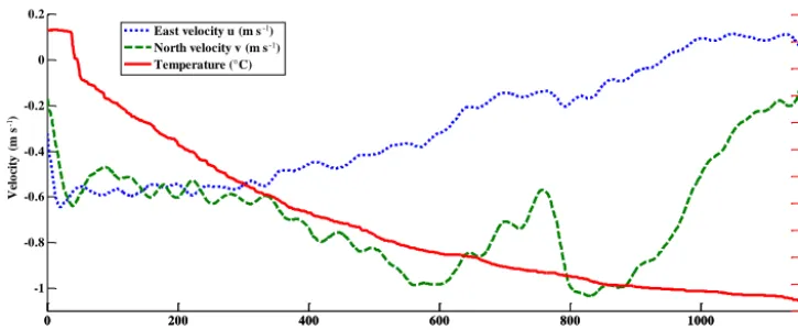
Figure 4.Ocean current velocity and temperature data as obtained using XCP probe (probe 1).
0 100 200 300 400 500 600
-1 -0.9 -0.8 -0.7 -0.6 -0.5 -0.4 -0.3 -0.2 -0.1 0
Depth (m)
V
el
oc
it
y (
m
s
-1)
ADCP east velocity (m s- 1) ADCP n orth velocity (m s- 1)
Figure 5.Ocean current velocity data (21◦59.420N, 118◦10.310E) as obtained using ADCP.
5. Based on the two components calculated above, the am-plitude, AF, and phase,ϕF, of the modulated signals
can be obtained: AF =
FI
2
+FQ
21/2
,
ϕF =tan−1
−FI
−FQ
F =AF6 ϕF. (32)
6. The amplitude and phase of the useful voltage signal and coil voltage signal are calculated using the proce-dure described in steps 3–5. It can be concluded that the amplitude and phase of the electric-field-related cur-rent signal and coil signal areFE=AE6 ϕEandFC=
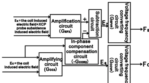
AC6 ϕC, respectively.
7. The circuit diagram of the hardware used for data pro-cessing is shown in Fig. 2. One can determine the orig-inal electric field and coil electric field as follows: EE=
FE
GEFVFGEF2−EC GCOR2
GEF2 ,
EC= FC
GCCVFGCC2
, (33)
where GEF2= E7
EE, GCOR2= E7
EC, GCC2=
E8 EC,
GEFVF=FE
E7(Hz/V ), andGCCVF= FC
E8(Hz/V ).
8. Calculate the northward speed and the eastward speed:
u= AE
FZL (1+K)
cosψ, (34)
v= − AE
FZL (1+K)
sinψ+W FH FZ(1+K)
, (35)
whereψ=3
2π+ϕC−ϕE.
Based on the velocity model, which usesW= −2×a×
t−b, the relation between the depth of the XCP probe in the ocean and time isZ= −1×(c+b×t+a×t2), wherea= −3.5×10⁻⁴,b=3.85, andc=3.1. This is the experience value of the development of the XCP probe.
3 Results and discussion
XCP in order to verify the accuracy of the proposed method for processing the XCP current data. An XCP probe (probe 1) was combined with an XCP buoy and released in the test area. The location of the release point was 21◦59.4200N, 118◦10.3100E, and data were collected up to a maximum depth of 1.151 m. The changes in the rotational frequency and coil signal (Ec) of the probe during sinking are shown in Fig. 3. The collected Ec data were processed to obtain the ocean current velocity data, which were then combined with the collected temperature data to plot the curves shown in Fig. 4.
The data shown in Figs. 4 and 5 were collected at a loca-tion 44.3◦ east by south of Shantou, Guangdong Province, China, and approximately 215 km away from Shantou, Guangdong Province, China. For comparison, Fig. 5 shows the ocean current velocity data as measured by an acoustic Doppler current profiler (ADCP) (Zoltan, 2012). The ADCP used was an OS-75K ADCP supplied by RDI and had a maximum profiling depth of 700 m (Liu, 2016). A compar-ison of Figs. 4 and 5 shows that the ocean current veloc-ity as measured by the XCP was generally consistent with that measured by the ADCP. From 16 m BSL to 600 m BSL, the velocity of the eastward ocean current changed gradually from−0.6 to−0.1 m s−1, while the velocity of the northward ocean current changed gradually from−0.5 to−0.96 m,s−1. The current at the top layer ran southwestward in a direc-tion approximately parallel to the coastal line in Guangdong Province, China.
4 Conclusions
Based on the theoretical principles underlying the process-ing of current data obtained usprocess-ing an XCP, in this study, we developed a method for processing XCP data in order to im-prove the accuracy of the measurements. In addition, a sea test was performed to evaluate the accuracy of the proposed method. Relationships derived based on theoretical studies were used to process the data collected from the sea test and to plot the current velocity data. Moreover, the current veloc-ity data obtained using the XCP were compared with those obtained using an ADCP. It was found that the trends in these two sets of velocity data were essentially consistent, confirm-ing the accuracy of the proposed method for processconfirm-ing XCP current data.
Data availability. No data sets were used in this article.
Competing interests. The authors declare that they have no conflict of interest.
Acknowledgements. This work was supported by the
Funda-mental Research Funds for the Central Universities of China (no. 2652014070), the National Natural Science Foundation of China (no. 41574131), and the National 863 Program of China (no. 2012AA061102).
Edited by: L. Vazquez
Reviewed by: two anonymous referees
References
Chave, A. D. and Luther, D. S.: Low frequency motionally-induced electromagnetic fields in the ocean, J. Geophys. Res., 95, 7185– 7200, 1990.
Chen, W. Y., Zhang, R., Liu, N., Zhang, M. M., and Tao, J. L.: Nu-merical simulation the flow field of expendable current profiler probe, Sci. Technol. Rev., 28, 62–65, 2010.
Chen, W. Y., Zhang, R., Liu, N., and Zhang, M. M.: Numerical study on the influence of rotating to the movement characteristics of XCP probe, Ocean Technol., 30, 61–63, 2011.
Crews, A. and Futterman, J.: Geomagnetic micropulsations due to the motion of ocean waves, J. Geophys. Res., 67, 299–306, 1962. Gandolfi, A., Nobili, C., Prudenziati, M., and Taroni, A.: Voltage-to-frequency conversion of signals supplied by physical-quantity sensors, IEEE T. Ind. El. Con. In., 4, 107–114, 1972.
Hisayoshi, S. and Hisashi, U.: Motional magnetotellurics by long oceanic waves, Geophys. J. Int., 201, 390–405, 2015.
Lim, Y. C. and Lian, Y.: The optimum design of one- and two-dimensional FIR filters using the frequency-response masking technique, IEEE Trans. Circuits Syst., 40, 88–95, 1993. Lin, C. S. and Ren, D. K.: Calculation of electromagnetic field
in-duced by ocean current, Journal of Naval University of Engineer-ing, 15, 19–22, 2003.
Liu, N. and He, H. K.: Study on the theory of expendable current profiler measurement, Ocean Technol., 29, 8–11, 2010. Liu, N., Li, Y. J., and Zhu, G. W.: A kind of fast expendable current
profiler measure production, Ocean Technol., 26, 27–31, 2007. Liu, Y. X.: Review on development of ADCP technology and its
application, Hydrographic Surveying and Charting, 36, 45–19, 2016.
Larsen, J. C. and Sanford, T. B.: Florida current volume transports from voltage measurements, Science, 227, 302–304, 1985. Wang, Y. B., Chen, W. D., and Du, Y.: Effect of ocean wave on
mag-nitude of underwater electromagnetic field, J. Trop. Oceanogr., 24, 37–40, 2005.
Wu, J. S. and Chen, Y.: Study on the waves by the electromagnetic field induced by the waves in the geomagnetic field, Mar. Sci. 6, 26–30, 1991.
Yan, X. W., Yan, H., and Xiao, C. H.: Research on model of induce magnetic vector of ocean waves, Hydrographic Surveying and Charting, 31, 8–11, 2011.
Zhang, Q. S., Deng, M., and Wang, Q.: Dynamic data transmission technique for expendable current profiler, Adv. Mat. Res., 220, 436–440, 2011.
Zhang, Z. L., Wei, W. B., Liu, B. H., Deng, M., and Jin, S.: The-oretical calculation of electromagnetic field generated by ocean waves, Acta Oceanol. Sin., 30, 42–46, 2008.