Some Sequence of Wrapped Δ Labellings for the Complete Bipartite Graph

http://dx.doi.org/10.4236/am.2015.61019

Some Sequence of Wrapped

Δ

-Labellings for

the Complete Bipartite Graph

Tomoko Adachi, Daigo Kikuchi

Department of Information Sciences, Toho University, Funabashi, Japan Email: adachi@is.sci.toho-u.ac.jp

Received 2 January 2015; accepted 17 January 2015; published 20 January 2015

Copyright © 2015 by authors and Scientific Research Publishing Inc.

This work is licensed under the Creative Commons Attribution International License (CC BY). http://creativecommons.org/licenses/by/4.0/

Abstract

The design of large disk array architectures leads to interesting combinatorial problems. Mini-mizing the number of disk operations when writing to consecutive disks leads to the concept of

“cluttered orderings” which were introduced for the complete graph by Cohen et al. (2001).

Muel-ler et al. (2005) adapted the concept of wrapped Δ-labellings to the complete bipartite case. In this

paper, we give some sequence in order to generate wrapped Δ-labellings as cluttered orderings

for the complete bipartite graph. New sequence we give is different from the sequences Mueller et

al. gave, though the same graphs in which these sequences are labeled.

Keywords

Cluttered Ordering, RAID, Disk Arrays, Label for a Graph

1. Introduction

The desire to speed up secondary storage systems has lead to the development of disk arrays which achieve per-formance through disk parallelism. While perper-formance improves with increasing numbers of disks, the chance of data loss coming from catastrophic failures, such as head crashes and failures of the disk controller electron-ics, also increases. To avoid high rates of data loss in large disk arrays, one includes redundant information stored on additional disks—also called check disks—which allows the reconstruction of the original data— stored on the so-called information disks—even in the presence of disk failures. These disk array architectures are known as redundant arrays of independent disks (RAID) (see [1] [2]).

utilizing the notion of a wrapped Δ-labelling. In the case of a complete tripartite graph, we refer to [10].

As Figure 1, we present the case =2. For example, information disk 1 is associated to the check disks a and c. A 2-dimensional parity code can be modeled by the complete bipartite graph K_{ ,} =

(

U V E, ,

)

in the following way. The point set of K_{ ,} is partitioned into the two sets—U and V both having cardinality . Assign the points of U to the  check bits corresponding to the rows and the points of V to the  check bits corresponding to the columns. By definition, in K_{ ,} any point of U is connected with any point of V exactly on edge constituting the edge set E, i.e., E =2 (see Figure 2).

In this paper, we make label to the vertex of a bipartite graph. For example, we make label 1, 3, 0 and −1, respectively, to four vertices a, b, c and d of a bipartite graph in Figure 2. By such labelling, we get that the label of the edge

{ }

a c, is 1 0− =1; the label of the edge

{ }

a d, is 1− − =

( )

1 2; the label of the edge

{ }

b c, is 3 0− =3 and the label of the edge

{ }

b d, is 3− − =

( )

1 4. The labellings

[ ]

1, 3 of the upper vertices

[ ]

a b, and the labellings

[

0, 1−

]

of the lower vertices

[ ]

c d, are sequences. The goal of this paper is to find new sequence in order to generate wrapped Δ-labellings as cluttered orderings for the complete bipartite graph. In Section 5, we give new sequence which we want. The new sequence we give is different from the sequences Mueller et al. [9] gave, though the same graphs in which these sequences are labeled.

2. A Cluttered Ordering

In a RAID system disk writes are expensive operations and should therefore be minimized. In many applications there are writes on a small fraction of consecutive disks—say d disks—where d is small in comparison to k, the number of information disks. Therefore, to minimize the number of operations when writing to d consecutive information disks one has to minimize the number of check disks—say f—associated to the d information disks.

Let G=

(

V E,

)

be a graph with n= V vertices and edge set E=

{

e e₀, ,₁,em−₁

}

. Let d≤m be a

positive integer, called a window of G, and π a permutation on

{

0,1,,m−1

}

, called an edge ordering of G. Then, given a graph G with edge ordering π and window d, we define V_iπ,d to be the set of vertices which are connected by an edge of

{

e_{π( )i},e_{π( )i+1},,e_{π(i d+ −1)}

}

, 0≤ ≤ −i m 1, where indices are considered modulo m. The cost of accessing a subgraph of d consecutive edges is measured by the number of its vertices. An upper

bound of this cost is given by the d-maximum access cost of G defined as ,

maxiVi d

π _{. An ordering π is a (d,}

f)-cluttered ordering, if it has d-maximum access cost equal to f. We are interested in minimizing the parameter f.

Let  be a positive integer and let K_{ ,} denote the complete bipartite graph with 2 vertices and 2 edges. In the following, we identify the vertex set of K_{ ,} with Z_×Z₂, where two vertices are connected by an edge iff they have different second components in Z_×Z₂. The construction of (d, f)-cluttered orderings for

,

K_{ } with small positive integer f is based on two fundamental concepts. Firstly, we introduce the well-known concept of a Δ-labelling of a suitable bipartite subgraph from which one gets a decomposition of K_{ ,} into isomorphic copies of this subgraph. Secondly, we define the concept of a (d, f)-movement which will lead to “locally” defined edge orderings of K_{ ,} . This principle was implicitely used in [6] in case of the complete graph. In case of the complete bipartite graph, we refer to [9].

[image:2.595.176.457.559.620.2]

In the following, H =

(

U E,

)

always denotes a bipartite graph with vertex set U which is partitioned into

Figure 1. 2-dim. parity code and its parity check matrix.

two subsets denoted by V and W. Any edge of the edge set E contains exactly one point of V and W respectively. Let = E , then a Δ-labelling of H with respect to V and W is defined to be a map ∆:U→Z_×Z₂ with

( )

V Z

{ }

0

∆ ⊂ _× and ∆

( )

W ⊂Z_×

{ }

1 , where each element of Z_ occurs exactly once in the difference list

( )

E :

(

π

1

(

( ) ( )

v w

)

v V w W v w, ,

( )

, E

)

.

∆ = ∆ − ∆ ∈ ∈ ∈ (1)

Here, π₁:Z_×Z₂ →Z_ denotes the projection on the first component. In general, Δ-labellings are a well- known tool for the decomposition of graphs into subgraphs (see [11]). In this context a decomposition is un-derstood to be a partition of the edge set of the graph. In case of the complete bipartite graph, one has the fol-lowing proposition.

Proposition 1. ([9]) Let H=

(

U E,

)

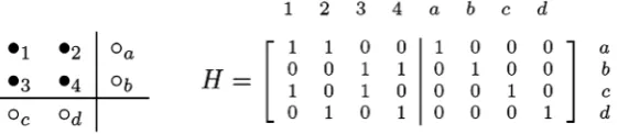
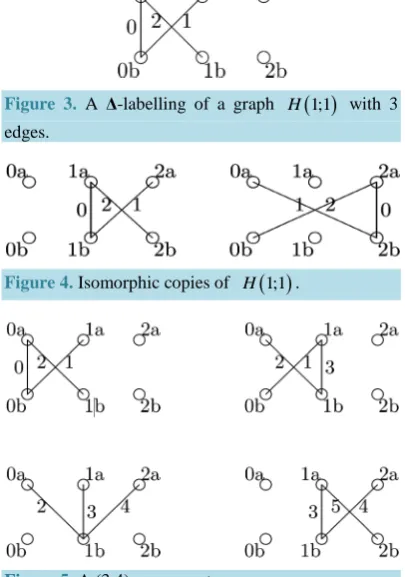
be a bipartite graph, = E , and Δ be a Δ-labelling as defined above. Then there is a decomposition of the complete bipartite graph K_{ ,} into isomorphic copies of H.

For example, Figure 3 shows Δ-labellings of a graph H=H

( )

1;1 with 3 edges leading to a decomposition of K_3,3 into isomorphic copies of H

( )

1;1 such as Figure 4. Next, in order to move a graph H to an isomorphic copy such as Figure 5, we define the concept of a (d, f)-movement which can easily be generalized to arbitrary set system.

Definition 1. Let G be a graph with edge set E G

( ) {

= e e₀, ,₁,en−₁

}

, where n is positive integer, and let Σ0,

( )

1 E G

Σ ⊂ with d:= Σ = Σ_{0 1} . For a permutation σ on

{

0,1,,n−1

}

define , 1 _{( )}

0

: d

d

i j i j

Vσ =



₌− e_{σ +} for 0≤ ≤ −i n d. Then, for some given a positive integer f, and a map σ is called a

(

d f,

)

-movement from Σ₀ to Σ₁ if Σ =₀

{

e_{σ( )j} 0≤ ≤ −j d 1

}

, Σ =₁

{

e_{σ( )j} n− ≤ ≤ −d j n 1

}

, and _max ,d

iVi f

σ _{≤ .}

In order to assemble such (d, f)-movements of certain subgraphs to a (d, f)-cluttered ordering, we need some notion of consistency. Let ϕ Σ → Σ: _{0 1} be any bijection, then a (d, f)-movement σ from Σ₀ to Σ₁ is called consistent with ϕ if

( )

( )

eσ j eσ(n d j) for j 0,1, ,d 1.

ϕ = _{− +} , = _ − (2)

[image:3.595.212.415.421.710.2]

Now, for each j∈Z_ one gets an automorphism τ_j of the bipartite graph K_{ ,} defined by cyclic transla-tion of the vertex set:

Figure 3. A Δ-labelling of a graph H

( )

1;1 with 3 edges.

Figure 4. Isomorphic copies of H

( )

1;1 .

( )

(

)

(

)

2 2

: , , : , ,

j Z Z Z Z j u b u j b

τ _× → _× τ = + (3)

( )

u b, ∈Z×Z2. Obviously, τj induces in a natural way an automorphism of the edge set of K , which we

also denote τ_j. Then, τ_j

( )

E( )i =E(i+j) and τ_j

( )

Σ( )₀i = Σ₀(i+j), i∈Z_. Next, we define a subgraph G( )0 ⊂K_{ ,} by specifying its edge set E G

( )

( )0 :=E( )0 ∪ Σ₀( )κ . Let E G

( )

( )0 =

{

e₀( ) ( )0,e₁0 ,,en( )0−₁

}

, n= + d, where we fix

some arbitrary edge ordering. We denote the restriction of the cyclic translation τ_κ to Σ( )₀0 by

ϕ

_κ( )0 which defines a bijection

ϕ

_κ( )0 :Σ → Σ( )₀0 ( )₀κ .

Definition 2. With above notation, a (d, f)-movement of G( )0 from Σ( )₀0 to Σ( )₀κ consistent with

ϕ

_κ( )0 will be denoted as

(

d f,

)

-movement from Σ( )₀0 consistent with the translation parameter

κ

.

According to Definition 1, such a (d, f)-movement is given by some permutation σ of the index set

{

0,1,,n−1

}

. By applying the cyclic translation τ_i one gets a graph G( )i :=τi

( )

G( )0 with edge set

( )

( )

( ) ( )

{

( ) ( ) ( )

}

0 0 , 1 , , 1

i i i i i i

n

E G =E ∪ Σ +κ = e e  e− , i∈Z. We denote the restriction of τκ to ( )0

i

Σ by

ϕ

_κ( )i which defines a bijection

( ) ( ) ( ) ( )

( )

( ) ( ) ( ) ( )

0 0 0

: , , .

i i i i i i i i

e e e

κ κ

κ κ

ϕ _{Σ → Σ} + ϕ ₌ + _{∈ Σ}

(4) Then σ also defines a

(

d f,

)

-movement of ( )i

G from Σ( )₀i to Σ(₀i+κ) consistent with

ϕ

_κ( )i . Using that

( ) ( ) ( )

0

i i

j

e_σ ∈ Σ , 0≤ <j d, (see Defintion 1), we get, for j=0,1,,d−1,

( ) ( )( ) ( ) ( ) ( )

( )

( ) ( ) ( ) ( ) ( ) 4 2 .

i i i i i

j j n d j j

e_σ+κ =ϕ_κ e_σ =e_{σ − +} =e_{σ +} (5)

Having such a consistent σ , it is easy to construct a (d, f)-cluttered ordering of K_{ ,} . In short, one orders the edges of K_{ ,} by first arranging the subgraphs of the decomposition along E( )0,E( )κ ,E( )2κ ,,E(( )−1κ) and then ordering the edges within each subgraph according to σ .

Proposition 2. ([9]) Let H =

(

U E,

)

, = E , be a bipartite graph allowing some ρ -labelling, and let

κ

be a translation parameter coprime to . Furthermore, let Σ ⊂₀ E, d:= Σ₀ . If there is a (d, f)-movement from Σ₀ consistent with

κ

, then there also is a (d, f)-cluttered ordering for the complete bipartite graph

 ,

K .

3. Construction of Cluttered Orderings of

H h t

( )

;

In this section, we define an infinite family of bipartite graphs which allow (d, f)-movements with small f. In order to ensure that these (d, f)-movements are consistent with some translation parameter

κ

, we impose an additional condition on the Δ-labellings also referred to as wrapped-condition.

Let h and t be two positive integers. For each parameter f and t, we define a bipartite graph denoted by

( ) (

; ,

)

H h t = U E . Its vertex set U is partitioned into U = ∪V W and consists of the following 2h t

(

+1

)

ver-tices:

(

)

{

}

(

)

{

}

: 0 1 ,

: 0 1 .

i i

V v i h t

W w i h t

= ≤ < + = ≤ < +

The edge set E is partitioned into subsets E_s, 0≤ <s t, defined by

{

}

{

}

{

}

{

}

{

}

{

}

1 0 : , , , : , , : , ,

: for 0 ,

: .

s i j

s i h j

s h i j

s s s s

t s s

E v w s h i j s h h

E v w s h j i s h h

E v w s h i j s h h

E E E E s t

E E

+

+

−

=

′ = ⋅ ≤ < ⋅ +

′′ = ⋅ ≤ ≤ < ⋅ +

′′′ = ⋅ ≤ ≤ < ⋅ +

′ ′′ ′′′

= ∪ ∪ ≤ <

=

_

Figure 6 shows the edge partition of H

( )

2;1 . For the number of edges holds

(

)

(

)

₍

₎

2 1 1

2 1

2 2

h h h h

E = ⋅t _h + + + + _=th h+

  .

The t subgraphs defined by the edge sets Es, 0≤ <s t, and its respective underlying vertex sets are isomorphic

to H h

( )

;1 . Intuitively speaking, the bipartite graph H h t

( )

; consists of t “consecutive” copies of H h

( )

;1 , where the last h vertices of V and W respectively of one copy are identified with the first h vertices of V and W respectively of the next copy. Traversing these copies with increasing s will define a (d, f)-movement of

( )

;

H h t with small parameter f as is shown in the next proposition.

Proposition 3. ([9]) Let h, t be pogitive integers. Let H h t

( ) (

; = U E,

)

, t≥2, be the bipartite graph as de- fined above. Then, there is a (d, f)-movement of H h t

( )

; from E₀ to E_t−₁ with d=h

(

2h+1

)

and f =4h.

By Proposition 1 a Δ-labelling of the graph H h t

( )

; will lead to a decomposition of the complete bipartite graph K_{ ,} into  isomorphic copies of H h t

( )

; , where =th

(

2h+1

)

. However, in general there is no

(

d f,

)

-movement consistent with some translation parameter

κ

. To this means, we impose an additional con-dition on the Δ-labelling. The following definition generalizes and adapts the notion of a wrapped Δ-labelling to the bipartite case, which was introduced in [6] for certain subgraphs of the complete graph.

Definition 3. Let H =

(

U E,

)

, = E , denote a bipartite graph and let X Y, ⊂U with X = Y . A Δ- labelling Δ is called a wrapped Δ-labelling of H relative to X and Y if there exists a

κ

∈Z coprime to  such that

( )

Y

( ) ( )

X κ, 0

∆ = ∆ + (6)

as multisets in Z_×Z₂. The parameter

κ

is also referred to as translation parameter of the wrapped

Δ-labelling.

For the graphs H =H h t

( )

; , we define X :=

{

v w_i, _i 0≤ <i h

}

and Y:=

{

v w ht_i, _i ≤ <i h t

(

+1

)

}

. Further-more, in the following we only consider wrapped Δ-labellings relative to X and Y for which the stronger condi-tion

(

vi ht+

)

( ) ( )

vi κ, 0 and

(

wi ht+

)

( ) ( )

wi κ, 0 ,

∆ = ∆ + ∆ = ∆ + (7)

hold for 0≤ <i h. Suppose we have such labelling Δ satisfying condition (7). Now, E( )i , i∈Z_, are isomor-phic copies of H h t

( )

; . Furthermore, Σ( )₀κ is isomorphic to H h

( )

;1 consisting of the first d edges of E( )κ . From condition (7) follows that the graph G( )0 ⊂K_{ ,} with edge set E G

( )

( )0 :=E( )0 ∪ Σ₀( )κ can obviously identified with H h t

(

; +1

)

. In addition, one easily checks that the (d, f)-movement of G( )0 =H h t

(

; +1

)

from Proposition 3 is consistent with the translation parameter

κ

.

Proposition 4. ([9]) Let h t be positive integers. From any wrapped , Δ-labelling of H h t

( )

; , satisfying condition (7), one gets a (d, f)-cluttered ordering of the complete bipartite graph K_{ ,} with =th

(

2h+1

)

,

(

2 1

)

d=h h+ , and f =4h.

4. Sequences of Wrapped

Δ

-Labellings for

H

(1;

t

),

H

(2;

t

) and

H

(

h

; 1)

In this section, we construct some infinite families of such wrapped Δ-labellings. By applying Proposition 2 we get explicite (d, f)-cluttered orderings of the corresponding bipartite graphs. For these results in this section, we refer to [9].

4.1. A Sequence for

H

(1;

t

)

We define a wrapped Δ-labelling of H

( )

1;t for any positive integer t. H

( ) (

1;t = U E,

)

has 2

(

t+1

)

vertices

and 3t edges. For a fixed t, we define ∆:U →Z₃t×Z₂ on the vertex set U= ∪V W as follows:

( )

(

₍

)

₎

(

)

(

)

(

)

2

2

, 0 , for 0 ,

1, 0 , for ,

1 ,1 , for 0 ,

( )

1,1 , for ,

j

j

jt j t

v

t j t

j t j t

w

t j t

≤ < 

∆ _{= }

+ =



 − ≤ <



∆ _{= }

+ =



where the integers in the first components are considered modulo 3t. We now compute the difference list ∆

( )

E

of δ defined as in (1). Hence each element of Z_3t appears in ∆

( )

E and the difference condition holds. Figure 3 illustrates the definition for the case t = 1.

Obviously, the wrapped-condition (7) relative to X =

{

v w₀, ₀

}

and Y =

{

v wt, t

}

holds as well and the

transla-tion parameter κ = +t2 1 is coprime to 3t for any t. Therefore, Δ defines the desired wrapped Δ-labelling of

( )

1;

H t .

Theorem 5. ([9]) Let t be a positive integer. For all t there is a (d, f)-cluttered ordering of the complete bi- partite graph K_3t,3t with d= 3 and f = 4.

Theorem 6. ([9]) Let t be a positive integer. For all t there is a (d, f)-cluttered ordering of the complete bi- partite graph K_{3 ,3t t} with d=3s+r and f =2

(

s+ +1

)

r, s>0, r=0,1, 2.

4.2. A Sequence for

H

(2;

t

)

We define a wrapped Δ-labelling of H

( )

2;t for any positive integer t. H

( ) (

2;t = U E,

)

has 4

(

t+1

)

ver-tices and 10t edges. For a fixed t, a labelling Δ is a map ∆:U→Z₁₀t×Z₂ on the vertex set U= ∪V W . We

specify the second component of Δ on the vertices V =

(

v v₀, ,₁ ,v₂t+₁

)

sequentially by the following list of 2t

+ 2 numbers:

0, 0 , ,1 1 , , j, j , , t1, t 1 , 0 , 0 ,

c c +a c c +a c c +a c₋ c₋ +a c +κ c + +a κ and, on the vertices W=

(

w w₀, ₁,,w₂t+₁

)

by, similarly,

0, 0 , 1, 1 , , j, j , , t 1, t1 , 0 , 0 ,

d d +b d d +b d d +b d₋ d₋ +b d +κ d + +b κ where we set

(

)

2

6 1, 2 , 0,1, , 1,

6 2, 2 1 , 0,1, , 1,

2 1.

j

j

a t c jt j t

b t d j t j t

t

κ

= − = = −

= − = − = −

= +

 

All integers are considered modulo 10t. Note that E =10t and κ =2t2+1 are coprime for all t and that the wrapped-condition (7) is obviously fulfilled. Thus, Δ defines a wrapped Δ-labelling.

Theorem 7. ([9]) Let t be a positive integer. For all t there is a (d, f)-cluttered ordering of the complete bipar- tite graph K_{10 ,10t t} with d=10 and f =8.

Theorem 8. ([9]) Let t be a positive integer. For all t there is a (d, f)-cluttered ordering of the complete bipar- tite graph K_{10 ,10t t} with d=10s+r and f =4

(

s+ +1

)

min

( )

r, 4 , s>0, r=0,1,, 9.

4.3. A Sequence for

H

(

h

; 1)

We define in this section a wrapped Δ-labelling for H h

( )

;1 for any positive integer h. H h

( ) (

;1 = U E,

)

has 4h vertices and h

(

2h+1

)

edges. We define the Δ-labelling ∆:U→Zh₍2h+1₎×Z2 on the vertex set U = ∪V W

by specifying the first component of Δ on the vertices V =

(

v v₀, ,₁,v₂h−₁

)

sequentially by the following list of

2h numbers:

0, 1, , h1, 0 , 1 , , h1 ,

a a  a− a +κ a +κ a− +κ

0, ,1 , h 1, 0 , 1 , , h 1 ,

b b  b₋ b +κ b +κ b₋ +κ

where we set

(

)

(

)

0

0

0, 2 2 1 , 1, 2, , 1,

0, 2 1 1, 1, 2, , 1,

1.

i j

a a i h i h

b b j h j h

κ

= = − + = −

= = − + − = −

= −

 

All integers are considered modulo h

(

2h+1

)

. Obviously, E =h

(

2h+1

)

and

κ

are coprime for any posi-tive integer h and the wrapped-condition (7) is fulfilled. Figure 7 illustrates the definition for the case h=3. All numbers in Z_h(2h+1) appear exactly once as difference of Δ which hence defines a wrapped Δ-labelling.

Theorem 9. ([9]) Let h be a positive integer. For all h there is a (d, f)-cluttered ordering of the complete bipartite graph K_{h(2h+1 ,) (h2h+1)} with d=h

(

2h+1

)

and f =4h.

5. Our Result: A Sequence of a Wrapped

∆

-Labelling for

H

( )

3;

t

In this section, we define a wrapped Δ-labelling of H

( )

3;t for any positive integer t. H

( ) (

3;t = U E,

)

has

(

)

6 t+1 vertices and 21t edges. For a fixed t, a labelling Δ is a map ∆:U→Z₂₁t×Z₂ on the vertex set

U = ∪V W. We specify the second component of Δ on the vertices V =

(

v v₀, ,₁ ,v₃t+₂

)

sequentially by the

following list of 3t+3 numbers:

0, 0 , 0 2 , ,1 1 , 1 2 , , j, j , j 2 , , t 1, t 1 , t 1 2 , 0 , 0 , 0 2 ,

c c +a c + a c c +a c + a c c +a c + a c₋ c₋ +a c₋ + a c +κ c + +a κ c + a+κ and, on the vertices W=

(

w w₀, ₁,,w₃t+₂

)

by, similarly,

0, 0 , 0 2 , 1, 1 , 1 2 , , j, j , j 2 , , t 1, t 1 , t 1 2 , 0 , 0 , 0 2 ,

d d +b d + b d d +b d + b d d +b d + b d₋ d₋ +b d₋ + b d +κ d + +b κ d + b+κ where we set

(

)

2

15 1 3 0,1, , 1,

15 2 3 1 0,1, , 1,

3 1.

j

j

a t c jt j t

b t d j t j t

t

κ

= − = = −

= − = − = −

= +

 

, ,

, ,

All integers are considered modulo 21t. Note that E =21t and 2 3t 1

κ = + are coprime for all positive

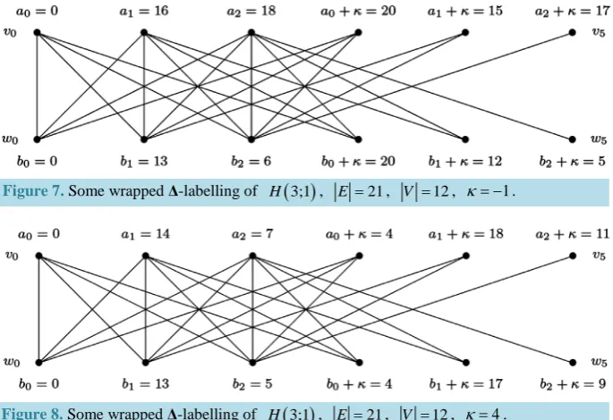
[image:7.595.142.485.480.715.2]

in-teger t and that the wrapped-condition (7) is obviously fulfilled. Figure 8 illustrates the definition for the case t = 1.

Figure 7. Some wrapped Δ-labelling of H

( )

3;1 , E =21, V =12, κ= −1.

We now compute the differences of Δ using the notation from (1):

( )

(

(

)

(

)

(

)

(

)

)

(

)

0 0 0 0 0 0 0 0 0 0 0 0 0 0 0

0 0 0 0

, , 2 2 , , 2 , , 2 ,

2 , 2

0,1, 2,15 1, 9 2, 6 2,12 4,15 , 6 3 ,

E c d c d a b c d a b c d a c d a c d b c d b

c d a b c d a b

t t t t t t

′ ∆ = − − + − − + − − + − + − − − − − + − − + − = − − + + +

( )

(

(

)

(

)

(

)

(

)

)

(

)

, , 2 2 , , 2 , ,

2 , 2 , 2

3 , 3 1, 3 2, 3 15 1, 3 9 2, 3 6 2, 3 12 4, 3 15 , 3 6 3

for

j j j j j j j j j j j j j

j j j j j j

E c d c d a b c d a b c d a c d a c d b

c d b c d a b c d a b

j j j j t j t j t j t j t j t

′

∆ = − − + − − + − − + − + − −

− − − + − − + −

= + + + − + − + + + + + + +

j=1, 2,,t−1,

( )

(

(

)

(

)

(

)

)

(

)

1 1 , 1 , 1 2 , 1 , 1 2 , 1 2 2

3 18 , 3 12 1, 3 6 2, 3 18 1, 3 12 , 3 18 2

for 1, 2, , 1,

j j j j j j j j j j j j j

E c d c d a c d a c d a b c d a b c d a b

j t j t j t j t j t j t

j t − − − − − − − ′′ ∆ = − − + − + − + − − + − − + − = + + − + − + + + + + =  −

( )

(

(

)

(

)

(

)

)

(

)

1 1, 1 , 1 2 , 1 , 1 2 , 1 2 2

3 3 3, 3 9 1, 3 15 1, 3 3 2, 3 9 , 3 3 1

for 1, 2, , 1,

j j j j j j j j j j j j j

E c d c d b c d b c d a b c d a b c d a b

j t j t j t j t j t j t

j t − − − − − − − ′′′ ∆ = − − − − − − + − − + − − + − = + − + − + + + − + + − = _ −

(

)

(

(

)

(

)

(

)

)

(

)

1 1 0 1 0 1 0 1 0 1 0

1 0

, , 2 , , 2 ,

2 2

18 1,12 2, 6 3,18 ,12 1,18 1 ,

t t t t t t

t

E c d c d a c d a c d a b c d a b

c d a b

t t t t t t

κ κ κ κ κ

κ − − − − − − − ′′ ∆ = − − − − + − − + − − + − − − + − − − + − = − − − − +

(

)

(

(

)

(

)

(

)

)

(

)

1 0 1 0 1 0 1 0 1 0 1

0 1

, , 2 , , 2 ,

2 2

6 2,12 ,18 2, 6 1,12 1, 6 .

t t t t t t

t

E c d c d b c d b c d a b c d a b

c d a b

t t t t t t

κ κ κ κ κ

κ − − − − − − − ′′′ ∆ = + − + − − + − − + − + − + − + − + − + − = − + − +

We now compute the difference list ∆

( )

E :

( ) (

E0′ 0,1, 2 ,

)

∆ ⊃ (1)

(

1

)

{

}

{

}

=1 3 , 3 1, 3 2 1 1 3, 4, 5, , 3 1 ,

t j

j E j j j j t t

− _′

∆

_

⊃ + + ≤ ≤ − =  − (2)

(

1

)

{

}

{

}

=1 3 3 3, 3 3 2, 3 3 1 1 1 3 , 3 1, 3 2, , 6 4 ,

t j

j E j t j t j t j t t t t t

− _′′′

∆



⊃ + − + − + − ≤ ≤ − = + +  − (3)

(

Et′′−1

) (

6t 3 ,

)

∆ ⊃ − (4)

(

Et′′′−1

) (

6t 2, 6t 1, 6 ,t

)

∆ ⊃ − − (5)

(

1

)

{

}

{

}

1

=1 3 6 2 1 6 1 ,

t j

j E j t j t

− −

′′

∆

_

⊃ + − = = + (6)

( ) ( ) (

E0′ 1 6t 2, 6t 3 ,

)

∆ − ⊃ + + (7)

(

1

)

( )

{

}

{

}

1

=1 6 3 6 2 2 1 6 4, 6 7, 6 10, , 9 5 ,

t j

j E j t j t t t t t

− −

′′

∆

_

− ⊃ + − ≤ ≤ − = + + +  − (8-1)

(

1

)

( )

{

}

{

}

=1 2 3 6 2, 3 6 3 1 2 6 5, 6 6, 6 8, 6 9, , 9 4, 9 3 ,

t j

j E j t j t j t t t t t t t

− _′

(

)

( )

(

)

(

(

)

( )

)

(

) (

)

{

} {

}

(

)

1 1 1

=1 6 1 2

8 1 8 2

3 6 2 2 1 3 6 2, 3 6 3 1 2

6 4, 6 5, 6 6, 6 7, 6 8, 6 9, 6 10, , 9 5, 9 4, 9 3 ,

t t

j j

j E j E

j t j t j t j t j t

t t t t t t t t t t

− − − = ′′ ′ ∆ − ∪ ∆ − ⊃ − ∪ − = + − ≤ ≤ − ∪ + + + + ≤ ≤ − = + + + + + + +  − − −





(8-3)

( ) ( ) ( ) (

E0′ 1 7 9t 2 ,

)

∆ − − ⊃ − (9)

(

1

)

( ) (

)

{

}

(

)

1 2 8 2 3 6 2, 3 6 3 1 9 1, 9 ,

t j

j E j t j t j t t t

− = ′

∆

_

− − − ⊃ + + + + = − = − (10)

(

1

)

( ) (

) ( )

{

}

(

)

1 2 8 2 10 3 9 2 1 1 9 1, 9 4, 9 7, ,12 5 ,

t j

j E j t j t t t t t

− = ′

∆

_

− − − − ⊃ + − ≤ ≤ − = + + + _ − (11-1)

(

1

)

( )

{

}

(

)

1

1 3 3 9 1, 3 9 1 1 9 2, 9 3, 9 5, 9 6, ,12 4,12 3 ,

t j

j E j t j t j t t t t t t t

− − = ′′′

∆

_

− ⊃ + − + ≤ ≤ − = + + + + _ − − (1 1-2)

(

)

( ) (

) ( )

(

)

(

(

)

( )

)

(

) (

)

{

} {

}

(

)

1 1 1

1 2 8 2 10 1 3

11 1 11 2

3 9 2 1 1 3 9 1, 3 9 1 1

9 1, 9 2, 9 3, 9 4, 9 5, 9 6, ,12 5,12 4,12 3 ,

t t

j j

j E j E

j t j t j t j t j t

t t t t t t t t t

− − − = ′ = ′′′ ∆ − − − − ∪ ∆ − ⊃ − ∪ − = + − ≤ ≤ − ∪ + − + ≤ ≤ − = + + + + + + _ − − −





(11-3)

(

Et′′−1

) ( ) (

4 12t 2,12t 1 ,

)

∆ − ⊃ − − (12)

(

Et′′′−1

) ( ) (

5 12 ,12t t 1 ,

)

∆ − ⊃ + (13)

(

1

)

( ) (

)

{

}

(

)

1

1 6 8 1 3 12 1, 3 12 1 12 2,12 3 ,

t j

j E j t j t j t t

− − = ′′

∆

_

− − − ⊃ + − + = = + + (14)

( ) ( ) ( ) ( ) (

E0′ 1 7 9 12t 4 ,

)

∆ − − − ⊃ + (15)

(

)

( ) (

) ( )

{

}

(

)

1 1

1 6 8 1 14 3 12 1, 3 12 2 1

12 5,12 6,12 8,12 9, ,15 4,15 3 ,

t j

j E j t j t j t

t t t t t t

− − = ′′

∆ − − − − ⊃ + − + ≤ ≤ −

= + + + + _ − −



_(16-1)

(

1

)

( ) (

) ( ) (

)

{

}

(

)

1 2 8 2 10 11 1 3 12 4 1 2 12 7,12 10, ,15 2 ,

t j

j E j t j t t t t

− = ′

∆

_

− − − − − − ⊃ + + ≤ ≤ − = + + _ − (16-2)

(

)

( ) (

) ( )

(

)

(

(

)

( ) (

) ( ) (

)

)

(

) (

)

{

} {

}

(

)

1 1 1

1 6 8 1 14 1 2 8 2 10 11 1 16 1 16 2

3 12 1, 3 12 2 1 3 12 4 1 2

12 5,12 6,12 7,12 8,12 9,12 10, ,15 4,15 3,15 2 ,

t t

j j

j E j E

j t j t j t j t j t

t t t t t t t t t

− − − = ′′ = ′ ∆ − − − − ∪ ∆ − − − − − − ⊃ − ∪ − = + − + ≤ ≤ − ∪ + + ≤ ≤ − = + + + + + + _ − − −





(16-3)

( ) ( ) ( ) ( ) ( ) (

E0′ 1 7 9 15 15t 1,15 ,t

)

∆ − − − − = − (17)

(

1

)

( ) (

) ( ) (

) (

)

{

}

(

)

1 2 8 2 10 11 1 16 2 3 12 4 1 15 1 ,

t j

j E j t j t t

− = ′

∆



− − − − − − − − ⊃ + + = − = + (18)

(

)

( ) (

) ( ) (

) (

) ( )

{

}

(

)

1

1 2 8 2 10 11 1 16 2 18

3 15 1, 3 15 1 1

15 2,15 3,15 5,15 6, ,18 4,18 3 ,

t j j E

j t j t j t

t t t t t t

(

1

)

( ) (

)

{

}

(

)

1

1 3 11 2 3 15 1 1 1 15 4,15 7, ,18 2 ,

t j

j E j t j t t t t

− − = ′′′

∆

_

− − − = + + ≤ ≤ − = + + _ − (19-2)

(

)

( ) (

) ( ) (

) (

) ( )

(

)

(

(

)

( ) (

)

)

(

) (

)

{

} {

}

(

)

1 1

1

1 2 8 2 10 11 1 16 2 18 1 3 11 2

19 1 19 2

3 15 1, 3 15 1 1 3 15 1 1 1

15 2,15 3,15 4,15 5,15 6,15 7, ,18 4,18 3,18 2 ,

t t

j j

j E j E

j t j t j t j t j t

t t t t t t t t t

− −

−

= ′ = ′′′

∆ − − − − − − − − − ∪ ∆ − − −

= − ∪ −

= + − + ≤ ≤ − ∪ + + ≤ ≤ −

= + + + + + +  − − −





(19-3)

(

Et′′−1

) ( ) ( ) (

4 12 18t 1,18 ,18t t 1 ,

)

∆ − − = − + (20)

(

Et′′′−1

) ( ) ( ) (

5 13 18t 2 ,

)

∆ − − = + (21)

( ) (

) ( ) (

)

{

}

(

)

1

1 1

6 8 1 14 16 1 3 18 , 3 18 1, 3 18 2 1 1

18 3,18 4,18 5, , 21 1 .

t j j

E j t j t j t j t

t t t t

− − =

 _′′ 

∆_{ }− − − − − − = + + + + + ≤ ≤ −

 

= + + +  −



₍₂₂₎

From this one easily checks that the twenty-two lists cover all numbers in Z_21t exactly once. Thus, Δ defines a wrapped Δ-labelling and by applying Proposition 4 we get the following result.

Theorem 10. Let t be a positive integer. For all t there is a (d, f)-cluttered ordering of the complete bipartite graph K_{21 ,21t t} with d=21 and f =12.

Using the same edge ordering of K_{21 ,21t t} one gets the following theorem by enlarging the window d.

Theorem 11. Let t be a positive integer. For all t there is a (d, f)-cluttered ordering of the complete bipartite graph K_{21 ,21t t} with d=21s+r and f =6

(

s+ +1

)

min

( )

r, 6 , s>0, r=0,1,, 20.

For example, we get a (21, 12)-cluttered ordering of K_{21 ,21t t}. For the graphs K_{21 ,21t t}, this is a much better ordering than the (21, 16)-cluttered ordering from Theorem 6.

6. Conclusion

In conclusion, we give a new sequence for construction of wrapped Δ-labellings.Figure 7and Figure 8 are the same as a graph, but they are different as a sequence. Cluttered orderings given by two sequences construct the different orderings for the complete bipartite graph K_21,21.

Acknowledgements

We thank the Editor and the referee for their comments.

References

[1] Hellerstein, L., Gibson, G., Karp, R., Katz, R. and Patterson, D. (1994) Coding Techniques for Handling Failures in Large Disk Arrays. Algorithmica, 12, 182-208. http://dx.doi.org/10.1007/BF01185210

[2] Chen, P., Lee, E., Gibson, G., Katz, R. and Ptterson, D. (1994) RAID: High-Performance, Reliable Secondary Storage. ACM Computing Surveys, 26, 145-185. http://dx.doi.org/10.1145/176979.176981

[3] Chee, Y., Colbourn, C. and Ling, A. (2000) Asymptotically Optimal Erasure-Resilient Codes for Large Disk Arrays. Discrete Applied Mathematics, 102, 3-36. http://dx.doi.org/10.1016/S0166-218X(99)00228-0

[4] Cohen, M. and Colbourn, C. (2000) Optimal and Pessimal Orderings of Steiner Triple Systems in Disk Arrays. Lecture Notes in Computer Science, 1776, 95-104. http://dx.doi.org/10.1007/10719839_10

[5] Cohen, M. and Colbourn, C. (2001) Ordering Disks for Double Erasure Codes. Proceedings of the Thirteenth Annual ACM Symposium on Parallel Algorithms and Architectures, 229-236.

[6] Cohen, M., Colbourn, C. and Froncek, D. (2001) Cluttered Orderings for the Complete Graph. Lecture Notes in Com-puter Science, 2108, 420-431. http://dx.doi.org/10.1007/3-540-44679-6_48

[7] Cohen, M. and Colbourn, C. (2004) Ladder Orderings of Pairs and RAID Performance. Discrete Applied Mathematics, 138, 35-46. http://dx.doi.org/10.1016/S0166-218X(03)00268-3

Sys-tem Science, 4, 750-754.

[9] Mueller, M., Adachi, T. and Jimbo, M. (2005) Cluttered Orderings for the Complete Bipartite Graph. Discrete Applied Mathematics, 152, 213-228. http://dx.doi.org/10.1016/j.dam.2005.06.005

[10] Adachi, T. (2007) Optimal Ordering of the Complete Tripartite Graph K9,9,9. Proceedings of the Fourth International

Conference on Nonlinear Analysis and Convex Analysis, 1-10.