https://doi.org/10.5194/gmd-12-1541-2019 © Author(s) 2019. This work is distributed under the Creative Commons Attribution 4.0 License.
The [simple carbon project] model v1.0
Cameron M. O’Neill, Andrew McC. Hogg, Michael J. Ellwood, Stephen M. Eggins, and Bradley N. Opdyke Research School of Earth Sciences, Australian National University, Canberra, Australia
Correspondence:Cameron O’Neill ([email protected]) Received: 12 July 2018 – Discussion started: 18 July 2018
Revised: 15 March 2019 – Accepted: 21 March 2019 – Published: 18 April 2019
Abstract. We construct a carbon cycle box model to pro-cess observed or inferred geochemical evidence from modern and paleo settings. The [simple carbon project] model v1.0 (SCP-M) combines a modern understanding of the ocean circulation regime with the Earth’s carbon cycle. SCP-M estimates the concentrations of a range of elements within the carbon cycle by simulating ocean circulation, biological, chemical, atmospheric and terrestrial carbon cycle processes. The model is capable of reproducing both paleo and mod-ern observations and aligns with CMIP5 model projections. SCP-M’s fast run time, simplified layout and matrix structure render it a flexible and easy-to-use tool for paleo and modern carbon cycle simulations. The ease of data integration also enables model–data optimisations. Limitations of the model include the prescription of many fluxes and an ocean-basin-averaged topology, which may not be applicable to more de-tailed simulations.
In this paper we demonstrate SCP-M’s application pri-marily with an analysis of the carbon cycle transition from the Last Glacial Maximum (LGM) to the Holocene and also with the modern carbon cycle under the influence of anthropogenic CO2 emissions. We conduct an atmospheric and ocean multi-proxy model–data parameter optimisation for the LGM and late Holocene periods using the grow-ing pool of published paleo atmosphere and ocean data for CO2,δ13C,114C and the carbonate ion proxy. The results provide strong evidence for an ocean-wide physical mech-anism to deliver the LGM-to-Holocene carbon cycle transi-tion. Alongside ancillary changes in ocean temperature, vol-ume, salinity, sea-ice cover and atmospheric radiocarbon pro-duction rate, changes in global overturning circulation and, to a lesser extent, Atlantic meridional overturning circulation can drive the observed LGM and late Holocene signals in atmospheric CO2,δ13C,114C, and the oceanic distribution ofδ13C,114C and the carbonate ion proxy. Further work is
needed on the analysis and processing of ocean proxy data to improve confidence in these modelling results.
1 Introduction
mod-els continue to be applied to resolve problems in the carbon cycle.
Our motivation in constructing a new box model of the full carbon cycle, the [simple carbon project] model v1.0 (SCP-M), is to contribute a simple, easy-to-use, open-access model implemented with freely available software, that is consistent with physical and biogeochemical oceanography, that caters for important features of the carbon cycle, and that has explicit avenues for data integration, optimisation and inversion. Recent advances in physical oceanography have refined our understanding of global ocean circulation and mixing fluxes. For example, Talley (2013) provided a simplified interpretation of the global ocean as a handful of large-scale processes, some of which are operating across all basins – as is the case with the global overturning circula-tion. De Boer and Hogg (2014) described a simple model of deep ocean mixing of water masses under the influence of sea-floor topography. These high-level concepts are easy to apply to box models. Furthermore, the growing pool of paleo proxy data across carbon isotopes and reconstructions (e.g. carbonate ion) presents an opportunity to progress model– data integrations using a number of different proxies. SCP-M caters for a range of proxies including the carbon isotopes and carbonate ion proxy, with the capacity for additional el-ements with minimal programming effort. The model–data experiment described in this paper provides a direct linkage between paleo data and discrete values for ocean parame-ters in the LGM and late Holocene periods, thus contribut-ing to our understandcontribut-ing of the LGM–Holocene carbon cy-cle transition. Combined with the expanding dataset of paleo observations, and with advances in computing power, data-aligned models such as SCP-M have the potential to improve our understanding of past changes in climate across many other time frames. Furthermore, there are a number of fea-tures of the carbon cycle outside ocean circulation and bi-ology which influence proxy indicators, particularly the car-bon isotopes. Omitting these features could lead to erroneous modelling outcomes, particularly in the case of the terrestrial biosphere, which strongly influences atmospheric CO2and δ13C (e.g. Francois et al., 1999). We compiled SCP-M to include a broad range of carbon cycle mechanisms, includ-ing carbonate production and dissolution, marine sediments, terrestrial biosphere, anthropogenic emissions sources, and continental weathering. Finally, SCP-M is computationally cheap and quick to run. A 10 000-year simulation takes ap-proximately 30 s to process on a regular laptop, enabling ex-haustive exploration of parameter space in optimisations that incorporate large datasets. While box models are not new, we argue that these features contribute to a new tool that is well-equipped to tackle a wide range of applications in pale-oceanography, paleoclimate and the modern carbon cycle.
In this paper we describe SCP-M and illustrate its appli-cation alongside LGM and late Holocene ocean and atmo-sphere data, with several insights for the transition between the two periods, plus modelling of the modern and future
car-bon cycle under the influence of anthropogenic emissions. Emphasis is placed on the model description and configura-tion.
2 SCP-M description
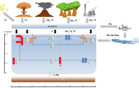
SCP-M is focussed on the ocean carbon cycle and is con-figured to estimate the time evolution of oceanic dissolved inorganic carbon (DIC) and its constituents: δ13C, 114C, plus alkalinity, phosphorus, oxygen, and atmospheric CO2, δ13C and114C. It contains a simple yet realistic represen-tation of large-scale ocean physical processes, with an over-lay of ocean chemistry and biology (Fig. 1). SCP-M simu-lates sources and sinks of carbon across the ocean and atmo-sphere, marine sediments, and terrestrial biosphere. Volcanic emissions, sedimentary weathering, rivers and anthropogenic emissions are prescribed fluxes. A range of carbon cycle fea-tures are included because the concentrations of carbon in the ocean and atmosphere (and its isotopes in particular) are sen-sitive to many sources and sinks, and omitting them makes it difficult to compare model results with the carbon data that indelibly feature their imprint. For example, regrowth in the terrestrial biosphere imparts a clear signature on the atmo-sphere and oceanδ13C data profile after the LGM (e.g. Fran-cois et al., 1999; Ciais et al., 2012; Hoogakker et al., 2016). In addition, the atmospheric radiocarbon source, marine sed-iments, volcanic emissions, continental weathering and now anthropogenic emissions exert important influences on car-bon cycle observations.
SCP-M was designed to compare model results with data and to solve for optimal parameter combinations. Within SCP-M, realistic implementation of physical processes upon a sound biogeochemical platform enables their transmission into paleo chemical tracer signals, for which proxy data ex-ist. Many of the key ocean physical and biological processes are prescribed in the model, allowing them to be free pa-rameters in model–data experiments. SCP-M itself is imple-mented with a matrix framework which enables more boxes to be added, ocean basins to be separated, elements to be added and exploration of a range of hypotheses, all with min-imal programming effort.
2.1 Model topology
The box model is mostly conceptual in nature and is designed to test high-level concepts. Therefore, excessive detail and complication are to be avoided. However, key processes that are critical to the validity of any hypothesis being tested must be represented as well as possible.
Figure 1.SCP-M: configured as a seven-box ocean model plus atmosphere with marine sediments, continents and the terrestrial biosphere. The exchange of elemental concentrations, e.g.Ci(i=1,7), occurs due to fluxes between boxes.91(red arrows) is global overturning circulation (GOC),92(orange arrows) is Atlantic meridional overturning circulation (AMOC),γ1(blue arrows between boxes 4 and 6) is deep–abyssal mixing,γ2(blue arrows between boxes 1 and 3) is low-latitude thermohaline mixing,Z(green downward arrows) is the biolog-ical pump,FCA(white downward arrows) is the carbonate pump,DCA(white squiggles) is carbonate dissolution andP (black, bidirectional arrows) is the air–sea gas exchange. Box 1: low-latitude–tropical surface ocean; box 2: northern surface ocean; box 3: intermediate ocean; box 4: deep ocean; box 5: Southern Ocean; box 6: abyssal ocean; box 7: subpolar southern surface ocean.
masses, circulation and mixing fluxes, including estimates of the present-day magnitudes of those fluxes. The Talley (2013) model builds on the models of Broecker (1991), Gor-don (1991), Schmitz (1996), Lumpkin and Speer (2007), Kuhlbrodt et al. (2007), Talley (2008), and Marshall and Speer (2012). Key features of the Talley (2013) model in-clude the following.
– Atlantic thermocline water moves north, ultimately reaching the North Atlantic, driven by advection and surface buoyancy changes. High-salinity North Atlantic Deep Water (NADW) forms in the north by cooling, densification and convection and then travels south to rise up into the Southern Ocean via wind-driven up-welling and Ekman flows, forming Lower Circumpolar Deep Water (LCDW). This water comprises the upper (orange arrows) Atlantic meridional overturning circu-lation (AMOC) in SCP-M (Fig. 1).
– A fraction of the upwelled LCDW sinks to become Antarctic Bottom Water (AABW) under the influence
of cooling and brine rejection, south of the Antarctic Circumpolar Current (ACC). AABW moves northward along the ocean floor via adiabatic advection (Talley, 2013) in all basins. It upwells into deep water in the Pacific and Indian oceans and also into NADW in the Atlantic via upwelling with diapycnal diffusion (Tal-ley, 2013). The combined LCDW–AABW–PDW–IDW– NADW global overturning circulation (GOC) is repre-sented by the red arrows in Fig. 1.
Wa-ter (SAMW) at the base of the subtropical thermocline (advection with surface buoyancy fluxes).
– Joined thermocline waters, AAIW–SAMW, and up-welled thermocline waters from the Pacific and Indian oceans form the upper-ocean transport moving towards the North Atlantic.
A key contribution of the Talley (2013) study is that GOC is the pre-eminent process in distributing water throughout the global oceans. Talley (2013) provided a 2-D “collapsed” interpretation of a 3-D ocean layout based on the observation that similar large-scale processes (i.e. GOC) operate in all three major ocean basins, and this interpretation can directly inform a box model topology. The Talley (2013) 2-D global ocean view used in SCP-M captures the features described above in a simple ocean box model format. Talley (2013) also provided observation-based estimates of the ocean trans-port fluxes, which are scaled according to their ocean basin domain. For example, the GOC and AABW formation pro-cess is common to all basins and thus accounts for the largest flux of 29 Sverdrups (Sv, 106m3s−1). The AMOC–NADW sinking cell is confined to the Atlantic Basin and represents a smaller flux (19 Sv) of water (Talley, 2013).
The SCP-M dimensions are designed to be consistent with measured estimates of the ocean surface area, average depth, and total ocean and atmosphere volumes. The model is di-vided into boxes according to latitude and depth, but not by longitude. Therefore, it does not distinguish between the At-lantic, Pacific and Indian basins and does not allow for com-positional variations with longitude. Each box has a surface area and depth (and therefore volume) and corresponds to a location in the global ocean with reference to latitude and average depth. It is simple to add more boxes to divide the model into ocean basins.
SCP-M contains seven ocean boxes as shown in Fig. 1. The rationale for dividing the ocean into boxes is that there are regions of the ocean that are relatively well-mixed, or at least similar in terms of their prevailing element flux be-haviour. For the depth of the surface boxes, this rationale conveniently translates to the maximum wintertime mixed layer depth (MLD) (e.g. Kara et al., 2003; de Boyer Mon-tegut et al., 2004). We choose a depth of 100 m for box 1, the low-latitude surface box, which is a reasonable approx-imation to the 20–150 m seasonally varying MLD for the middle and low latitudes estimated by de Boyer Montegut et al. (2004) and consistent with the depth of a similar box in the Toggweiler (1999) model. This box represents the photic zone over much of the ocean, from 40◦S to 40◦N. Craig (1957) estimated the depth of this layer as 75 m±25 m, a value used by Keeling and Bolin (1968) in their simple ocean box model. We choose 250 m of depth for the NADW box (box 2) and the subpolar surface box (box 7) as per Tog-gweiler (1999). These boxes are deeper than the low-latitude surface box (de Boyer Montegut et al., 2004) in order to cap-ture the regions of deepwater upwelling (subpolar Southern
Ocean) and convective downwelling (North Atlantic). The MLD in these regions can vary between 70 and >500 m of depth depending on seasonal variations (de Boyer Mon-tegut et al., 2004). An intermediate-depth box (3) resides be-low the be-low-latitude surface box and extends from 100 m to 1000 m of depth. This box captures northward-flowing AAIW and SAMW from upwelled NADW–PDW–IDW (e.g. Talley, 2013). Box 4 is the deep ocean box, extending from 1000 m to 2500 m of depth, and incorporates the upwelling abyssal waters in all basins and downwelled NADW. This water is channelled back to the surface in the subpolar sur-face box and the Southern Ocean box, as per the wind-driven upwelling of Morrison and Hogg (2013) and Talley (2013). The Southern Ocean box (5) extends from 80 to 60◦S and from the ocean surface to 2500 m of depth. This box encompasses the Southern Ocean, the ACC and deep-water formation from southward-flowing upwelled NADW– PDW–IDW (Talley, 2013). The abyssal box (6) extends the full range of the ocean, from 2500 to 4000 m of depth (our assumed average depth of the ocean). This box is the path-way for northward-flowing AABW and incorporates mixing with overlying deep water and advection–upwelling (Talley, 2013).
2.2 The model parameters, processes and equations 2.2.1 Basic features
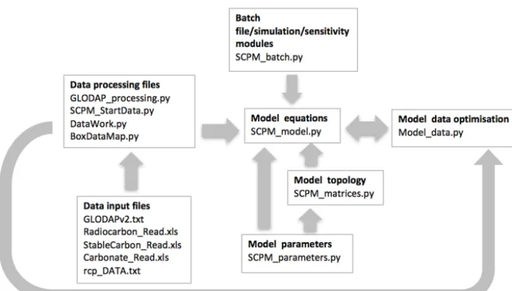
Figure 2 shows the suite of files used to execute SCP-M. We have chosen a modular approach to reduce the com-plexity of each of the model files. The SCP-M routine in-cludes data processing for the model’s boxes based on ge-ographic coordinates, model calibration to the data, model simulations, model–data optimisation, and charting and/or tabular output. SCP-M is implemented in Python 3.6, with the code and download (including user instructions) avail-able at https://doi.org/10.5281/zenodo.1310161 (O’Neill et al., 2018).
Figure 2.SCP-M Python and ancillary files with their linkages. Arrows refer to the direction of file linkages and the order of their activation during the routine of setting up and running the model. SCP-M is currently implemented in Python 3.6, although it has been run on other versions of Python. The folder or file structure separates model and data files. All files and user manuals are available from https://doi.org/ 10.5281/zenodo.1310161 (O’Neill et al., 2018).
2.2.2 The ocean circulation and mixing
There are four ocean physical parameters in SCP-M.91and 92are advection terms that represent the physical transport of water from one box to another, containing the element or species concentration of its box of origin.91represents GOC (e.g. Sarmiento and Toggweiler, 1984; Marshall and Speer, 2012; Talley, 2013) that infiltrates all basins (Talley, 2013) and is shown by the red arrows in Fig. 1. The91parameter allows variable allocation between transport from the deep ocean box (box 4) into the subpolar surface box (box 7) and directly into the polar box (box 5) via α.92represents the AMOC. This is the region of northward-flowing intermedi-ate wintermedi-aters in the Atlantic Ocean and the formation of NADW (Dickson and Brown, 1994; Talley, 2013), shown as orange arrows in Fig. 1.γ1andγ2are bidirectional mixing terms that exchange element or species concentrations between boxes without any net advection of water (blue arrows in Fig. 1).γ1 is bidirectional mixing between the deep and abyssal boxes of the form described by Lund et al. (2011) and De Boer and Hogg (2014).γ2is a low-latitude, intermediate–shallow box “thermocline” mixing parameter, which governs the con-stant bidirectional exchange between these two boxes (Liu et al., 2016).
The influence of each of the ocean parameters is pre-scribed in box model space by matrix equations, with one matrix for each parameter. Each row and column position in the matrix corresponds to a box location. The atmosphere box is treated separately from the ocean boxes, and it does not enter the ocean parameter matrices. The volumetric cir-culation or mixing parameters, in Sv, are multiplied by the
oceanic element concentration (mol m−3) to produce a mo-lar flux exchanged between ocean boxes. For example, the change in concentration of carbon (as DIC) in the deep box (box 4) from ocean physical parameters is estimated by
dC 4 dt
phys
= (1)
91(C6−C4) V4
+92(C2−C4) V4
+γ1(C6−C4) V4
,
whereCiis the concentration of DIC in each box in mol m−3 andVi is the volume of each box in m3. There is no vertical flux between box 4 and box 3 (intermediate box) in Eq. (1). We assume that this vertical flux is small compared with the lateral transport and compared with the mixing fluxes between boxes 4 and 6 (and boxes 1 and 3 in Eq. 2 be-low). We assume that the boundary between boxes 3 and 4 is the divide between northward-flowing water sourced from AAIW and SAMW, which overlies southward return flow from AMOC and PDW–IDW. The fluxes out of box 4 are shown by the terms−91C4,−92C4 and−γ1C4, with the fluxes into boxes 5, 6 and 7 treated in the equations for those boxes. For the low-latitude surface box (box 1),
dC 1 dt
phys
=γ2(C3−C1) V1
. (2)
We assume that lateral transport of northward-flowing water underlies box 1, involving box 7 (subpolar Southern Ocean), box 3 and box 1 (northern ocean). This intermediate-depth water is colder and denser than the overlying mixed layer, given its provenance of AAIW, SAMW and deep-upwelled NADW–PDW–IDW (Talley, 2013). These ocean circulation and mixing operations (e.g. Eqs. 1 and 2) can be vectorised for all boxes using sparse matrices, as follows.
dC
dt
phys
=(91T1+92T2+γ1E1+γ2E2)·C
V (3)
where
C=Ci,for i=1,7 (4)
V =Vi, for i=1,7 (5)
andT1,T2,E1andE2are sparse matrices defined as
T1=
0 0 0 0 0 0 0
0 0 0 0 0 0 0
0 0 0 0 0 0 0
0 0 0 −1 0 1 0
0 0 0 (1−α) −1 0 α
0 0 0 0 1 −1 0
0 0 0 α 0 0 −α
(6)
T2=
0 0 0 0 0 0 0
0 −1 1 0 0 0 0
0 0 −1 0 0 0 1
0 1 0 −1 0 0 0
0 0 0 0 0 0 0
0 0 0 0 0 0 0
0 0 0 1 0 0 −1
(7)
E1=
0 0 0 0 0 0 0
0 0 0 0 0 0 0
0 0 0 0 0 0 0
0 0 0 −1 0 1 0
0 0 0 0 0 0 0
0 0 0 1 0 −1 0
0 0 0 0 0 0 0
(8)
E2=
−1 0 1 0 0 0 0
0 0 0 0 0 0 0
1 0 −1 0 0 0 0
0 0 0 0 0 0 0
0 0 0 0 0 0 0
0 0 0 0 0 0 0
0 0 0 0 0 0 0
(9)
Given that we have applied the global ocean interpretation of Talley (2013) to the SCP-M layout, we have also adopted the observationally based estimates for the large-scale ocean fluxes for the modern ocean from the same study: GOC (91, 29 Sv), AMOC (92, 19 Sv) and deep–abyssal mixing (γ1, 19 Sv). For thermocline mixing between boxes 1 and 3 (γ2), we have adopted the value for the corresponding flux from Toggweiler (1999) of 40 Sv.
2.2.3 Biological flux parameterisation
The biological pump (e.g. Broecker, 1982) is a descriptor of marine biological activity, whereby organisms consume trients in shallow waters, die, sink and then release those nu-trients at depth. For example, carbon is taken up by shallow-water-dwelling phytoplankton through photosynthesis and then sequestered in deeper waters after sinking, breaking down and remineralising their nutrient load back into the wa-ter column. Volk and Hoffert (1985) made the distinction be-tween the soft tissue pump (STP) for soft-tissued organisms and the carbonate pump (carbonate-shelled organisms). We also distinguish between the two pumps, as they have differ-ent effects on carbon and alkalinity balances and therefore
pCO2and carbonate dissolution. This section deals with the STP, and a following section deals with the carbonate pump. Most STP organic matter is remineralised in the shallow to intermediate ocean depths, leading to a decrease in the ex-port of carbon as depth increases. According to Henson et al. (2011), only∼15 %–25 % of organic material is exported to
>100 m of depth, with most recycled in the shallower wa-ters.
Martin et al. (1987) modelled the soft-bodied organic flux of carbon observed from sediment traps in the north-east Pacific to create a simple power rule which is eas-ily applicable to modelling. The Martin et al. (1987) equa-tion produces a flux of organic carbon, which is a func-tion of depth from a base organic flux at 100 m of depth (the “Martin reference depth”). The flux at 100 m of depth was estimated by Martin et al. (1987) to be between 1.2 and 7.1 mol C m−2yr−1 from eight station observations in the northeast Pacific Ocean. Sarmiento and Gruber (2006) estimated a range of 0.0–5.0 mol C m−2yr−1, with some lo-calised higher values, across the global ocean. Equation (10) shows the general form of the Martin et al. (1987) equation:
F =F100 z
100
b
, (10)
whereF is a flux of carbon in mol C m−2yr−1,F
subsurface ocean box receives a flux of carbon from the box above it, at its ceiling depth (also the floor of the overly-ing box), and loses carbon as a function of the depth of the bottom of the box. Remineralisation in each box is accounted for as the difference between the influx and outflux of organic carbon. The biological flux out of the surface box 1 is shown by dC 1 dt bio = Z1S1
d f1 d0 b V1 , (11)
whereZ1is the biological flux of carbon prescribed for sur-face box 1 in mol C m−2yr−1,S1is the surface area of sur-face box 1,d0is the reference depth of 100 m for theZ pa-rameter value (Martin et al., 1987), and dc anddf are the ceiling and floor depths of a box, respectively. The dimen-sionless parameterbis the depth power function of the Mar-tin et al. (1987) equation, which tapers biological production and export below depths of 100 m. The net biological flux for intermediate-depth box 3 is given by
dC3 dt
bio
= Z1S1
d
c3 d0
b
−df3 d0
b
V3
. (12)
The process is vectorised using sparse matrices in the follow-ing:
dC
dt
bio
=ZS·(Bout+Bin)
V , (13)
where Z is an array of theZi (i=1,7) parameter, which varies across the surface boxes, andSis the array of surface box surface areasSi(i=1,7). As with the ocean parameters, the biological flux of carbon is divided by the box volume arrayV to return concentrations in mol m−3.Bout andBin
are sparse matrices as follows.
Bout= (14)
− df1 d0 −b
0 0 0 0 0 0
0 −
df2
d0 −b
0 0 0 0 0
−df3
d0 −b
0 0 0 0 0 0
−df4
d0 −b
−df4
d0 −b
0 0 0 0 −df4
d0 −b
0 0 0 0 −
df5
d0 −b
0 0
0 0 0 0 0 0 0
0 0 0 0 0 0 −df7
d0 −b
Bin= (15)
0 0 0 0 0 0 0
0 0 0 0 0 0 0
dc3 d0
−b
0 0 0 0 0 0
dc4 d0 −b dc4 d0 −b
0 0 0 0 dc4
d0 −b
0 0 0 0 0 0 0
dc6 d0 −b dc6 d0 −b
0 0 dc6 d0
−b
0 dc6 d0
−b
0 0 0 0 0 0 0
The value of the parameterZ in each surface box is speci-fied to vary as a fraction of the global value forZin SCP-M (presently 5.0 mol C m−2yr−1). There are higher fractions in the northern and southern oceans and smaller fractions in the low-latitude and polar oceans (e.g. Sarmiento and Gruber, 2006). During the model set-up we manually tuned the in-dividual surface box values by multiplying the global value forZby a scalar unique to each box. The values were tuned to align the model’s output with GLODAPv2 data for DIC, phosphorous, alkalinity, the carbonate ion and carbon iso-topes in each of the ocean boxes (Table 1). The resulting range for Z (1.1–5.33 mol C m−2yr−1) compares with the observations-based range of Martin et al. (1987) of 1.2– 7.1 mol C m−2yr−1and Sarmiento and Gruber (2006) of 0– 5 mol C m−2yr−1. We chose a value for the dimensionless b depth decay parameter of 0.75, which falls in the range of Gloege et al. (2017) of 0.68–1.13 and the error range of Berelson (2001) of 0.82±0.16. We found a global value of 0.75 to produce a better fit to the GLODAPv2 data when cal-ibrating the model. The biological flux of other elements and species, such as phosphorous and alkalinity, are calculated from the biological carbon flux using so-called Redfield ra-tios (e.g. Redfield et al., 1963; Takahashi et al., 1985; Ander-son and Sarmiento, 1994).
2.3 pCO2and carbonate
Modelling air–sea gas exchange, atmosphericpCO2and the “carbonate pump” rests on a realistic estimation ofpCO2in the ocean. For example, only a fraction of DIC in seawater can exchange with the atmosphere, and this fraction is es-timated by the oceanicpCO2. DIC itself consists of three major constituents: carbonic acid, bicarbonate and carbon-ate. Their relative proportions depend on total DIC, alkalin-ity, pH, temperature and salinity (Zeebe and Wolf-Gladrow, 2001).
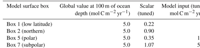
Table 1.Values for theZbiological production parameter (at 100 m of ocean depth) used in the SCP-M model calibration. A global value forZwas tuned in each surface box using scalars (column 3) to yield unique values for each surface box (column 4).
Model surface box Global value at 100 m of ocean Scalar Model input (tuned) depth (mol C m−2yr−1) (tuned) mol C m−2yr−1
Box 1 (low latitude) 5.0 0.22 1.1
Box 2 (northern) 5.0 0.90 4.5
Box 5 (polar) 5.0 0.35 1.75
Box 7 (subpolar) 5.0 1.07 5.33
run. This was demonstrated by Follows et al. (2006) to be sufficiently accurate for modelling purposes. The calculation takes inputs of DIC, alkalinity, temperature, salinity, phos-phorous and silicate to estimatepCO2.
Solving forpCO2enables the calculation of the concentra-tions of the three species of DIC, which further enables esti-mation of the dissolution and burial of carbonate in the wa-ter column and sediments. The latwa-ter is an important part of the oceanic carbon and alkalinity cycles and provides impor-tant feedbacks to atmospheric CO2on 1000-year time frames (e.g. Farrell and Prell, 1989; Anderson et al., 2007; Mekik et al., 2012; Yu et al., 2014b).
2.3.1 The carbonate pump
According to Emerson and Hedges (2003),∼20 %–30 % of CaCO3formed in the ocean’s surface is preserved in ocean floor sediments, with the rest dissolved in the water column. Klaas and Archer (2002) estimated that 80 % of the organic matter fluxes in the ocean below 2000 m are driven by or-ganic matter associated with carbonate ballast. Therefore, the so-called “carbonate pump” is a relatively efficient transport of carbon and alkalinity in the ocean. According to Farrell and Prell (1989), the carbonate pump is a dynamic process, and the dissolution and burial in sediments of CaCO3is ob-served to vary across (and within) glacial–interglacial cycles. To replicate this flux of carbon and alkalinity, a term is added to the carbon cycle equation to represent the flux of calcium carbonate (shells) out of the surface boxes into the abyssal box and sediments. This is an extension of the sur-face organic carbon flux Z described in Eq. (13) via the “rain ratio” parameter. The rain ratio is a common term in ocean biogeochemistry (e.g. Archer and Maier-Reimer, 1994; Ridgewell, 2003) and refers to the ratio between shell-based “hard” carbon and organic “soft” carbon fluxes in the biologically driven rain of carbon from the ocean’s surface. Sarmiento et al. (2002) estimated a global average value for the rain ratio of 0.06±0.03, with local maxima and minima of 0.10 and 0.02, respectively, providing a narrow range of global values. We apply the rain ratio as a parameter multi-plied by the organic flux parameter Z. We chose an initial value of 0.07, which provided appropriate values for DIC, alkalinity and dissolution in the model’s boxes during the model spin-up (with reference to GLODAPv2 data). The
combination delivers the physical production and export of calcium carbonate at the Martin reference depth (100 m).
sed-iments via undersaturation-driven dissolution in the abyssal water overlying the sediments.
The net flux of carbonate between ocean boxes and out of the ocean and into the sediments is shown in vectorised Eq. (16):
dC
dt
carb
=(FCAZS)
V +(ζ+)CaCO3, (16) where FCA is the rain ratio, ζ is the constant background dissolution rate,is the saturation-state-dependent dissolu-tion funcdissolu-tion of Morse and Berner (1972) and Millero (1983), and CaCO3is the concentration of calcium carbonate in each box. The dissolution equation of Morse and Berner (1972) operates on CaCO3, which is calculated by multiplying Ca by CO23−, where Ca is estimated from salinity in each box as per Sarmiento and Gruber (2006).
2.3.2 Air–sea gas exchange
CO2 is transported across the air–sea interface by gaseous exchange. According to Henry’s law, the partial pressure of a gas [P] above a liquid in thermodynamic equilibrium will be directly proportional to the concentration of the gas in the liquid:
[P] =KHC, (17)
whereKHis the solubility of a gas in mmol m−3atm−1andC is its concentration in the liquid. Many ocean models specify the air–sea gas exchange of CO2as a function of thepCO2 differential between ocean and atmosphere, a CO2solubility coefficient (e.g. Weiss, 1974), and a so-called “piston” or gas transfer velocity, which governs the rate of gas exchange, in m s−1(e.g. Toggweiler, 1999; Zeebe, 2012; Hain et al., 2010; Watson et al., 2015). We adopt the same approach in esti-mating the exchange of CO2between a surface box and the atmosphere:
dC 1 dt
gas
=P1S1K01 pCO2at−pCO21
ρ, (18)
whereP1is the piston velocity parameter in box 1 in m s−1. P is allowed to vary in each surface box, enabling scenario analysis such as the variation of sea-ice cover in the polar box (e.g. Stephens and Keeling, 2000; Ferrari et al., 2014).
K01 is the solubility of CO2 in mol kg
−1atm−1 (Weiss, 1974), subsequently converted into mol m−3by multiplying by seawater densityρ.pCO21and pCO2atare the partial pres-sures of CO2in surface ocean box 1 and the atmosphere, re-spectively, in ppm. The equation is vectorised as follows:
dC
dt
gas
=P SK0 pCO2at−pCO2
ρ, (19)
where P =Pi (i=1,7), with zero values for non-surface boxes, andK0=K0i (i=1,7).
2.4 Sea surface temperature and salinity
Ocean box temperature and salinity are forced in SCP-M, not calculated by the model. Each box has a prescribed value for temperature and salinity, which can be time dependent. During initialisation, the model takes box-averaged values for temperature and salinity from the GLODAPv2 database. The values can be varied between model experiments, for example Holocene versus LGM reconstructions. We argue that this approach is plausible given the availability of tem-perature and salinity proxy–data inputs for a range of paleo (e.g. Adkins et al., 2002; Kohfeld and Chase, 2017), mod-ern (e.g. Olsen et al., 2016) and future scenarios (e.g. IPCC, 2013a). For the modern and future scenarios (Sect. 3.3), we forced temperature with time series data and projections. The temperature and salinity values feed into the calculations for oceanpCO2, which further enables the calculation of air–sea gas exchange and the species of DIC in seawater (H2CO3, HCO3−and CO23−).
2.5 Atmosphere and terrestrial carbon cycle
SCP-M incorporates the terrestrial biosphere, continental weathering and river run-off into the ocean, plus an atmo-spheric radiocarbon source and volcanic and industrial emis-sions.
V is a constant prescribed flux of volcanic emissions of CO2 in SCP-M. Toggweiler (2008) estimated this volcanic flux of CO2 emissions at 4.98×10¹²mol yr−1 using a car-bon cycle model which balanced volcanic emissions with land-based weathering sinks. The weathering of carbonate and silicate rocks also creates DIC and alkalinity run-off into rivers, which finds its way into the ocean (Amiotte Suchet et al., 2003). Relative alkalinity and DIC concentrations af-fect ocean pCO2 and carbonate ion levels, which impacts atmospheric CO2and the dissolution and burial of carbon-ates (Sarmiento and Gruber, 2006). We apply the approach of Toggweiler (2008), whereby silicate and carbonate weath-ering fluxes of DIC and alkalinity enter only the low-latitude surface ocean box (box 1):
d C1 dt
weath
=(WSC+(WSV+WCV)AtCO2), (20)
where WSC is a constant silicate weathering term set at 0.75×10⁻⁴mol m−3yr−1, WSV is a variable rate of sili-cate weathering per unit of atmosphere CO2 (ppm) set to 0.5 mol m−3atm−1 CO
2yr−1 andWCV is the variable rate of carbonate weathering with respect to atmosphere CO2set at 2 mol m−3atm−1CO2yr−1(Toggweiler, 2008).
Equation (20) is vectorised by multiplying by a vector of boxes with only a non-zero value for box 1.
The terrestrial biosphere may act as a sink of CO2during periods of biosphere growth (e.g. post-glacial regrowth), via carbon fertilisation, or a source of CO2(e.g. glacial reduc-tion) via respiration. We employ a two-part model of the ter-restrial biosphere with a long-term (woody forest) and short-term (grassland) terrestrial biosphere box as described by Raupach et al. (2011) and Harman et al. (2011), with net pri-mary productivity (NPP) and respiration parameters control-ling the balance between the uptake and release of carbon. NPP is positively affected by atmospheric CO2, the so-called “carbon fertilisation” effect (e.g. Raupach et al., 2011). Res-piration is assumed proportional to the carbon stock. The bio-sphere also preferentially partitions the lighter carbon isotope 12C, leading to a relative enrichment inδ13C in the atmo-sphere during net uptake of CO2. The change in atmospheric CO2from the terrestrial biosphere in the model is given by dAtCO 2 dt NPP = (21)
−NpreRP
1+βLN
AtCO 2 AtCO2pre
+Cstock1 k1
+Dforest,
where Npre is NPP at a reference level (“pre”) of atmo-spheric CO2, and RP is the parameter to split NPP between the short-term terrestrial biosphere carbon stock (fast respi-ration) and the long-term stock (slow respirespi-ration) (Raupach et al., 2011). β is the parameterisation of carbon fertilisa-tion, which causes NPP to increase (decrease) logarithmi-cally with rising (falling) atmospheric CO2levels, and has a typical value of 0.4–0.8 (Harman et al., 2011).Cstock1is the short-term carbon stock andk1is the time frame for respira-tion in the short-term carbon stock (in years). For the long-term terrestrial biosphere, we substitute(1−RP)in place of RP and Cstock2 and k2 for the long-term carbon stock and respiration rate, respectively. Dforest is a prescribed flux of deforestation emissions, which can be switched on or off in SCP-M. Aδ13C fractionation factor is applied to the terres-trial biosphere fluxes of carbon, effecting an increase in at-mosphericδ13C from biosphere growth and a decrease from respiration.
2.6 The complete carbon cycle equations
Equation (22) shows the full vectorised model equation for the calculation of the evolution of carbon concentration in the ocean boxes, incorporating Eqs. (1)–(21).
d(C)
dt = (22)
dC dt phys + dC dt bio + dC dt carb + dC dt gas + dC dt weath
The calculation of atmospheric CO2is dAtCO2
dt =
dAtCO 2 dt gas + dAtCO 2 dt NPP (23) + dAtCO 2 dt volcs + dAtCO 2 dt weath + dAtCO 2 dt anth ,
where the additional term hdAtCO2 dt
i
anth consists of a pre-scribed flux ofδ13C-depleted and14C-dead CO2to the atmo-sphere from human industrial emissions, which is activated by a model switch in SCP-M.
2.7 Treatment of carbon isotopes
Carbon isotopes are an important component in SCP-M be-cause they are key sources of proxy data. Carbon isotope fluxes are treated largely the same as DIC in SCP-M, with minor modification. For example, carbon isotopes are typi-cally reported in delta notation (δ13C and114C), which is the ‰ deviation from a standard reference value in nature. SCP-M operates with a metric mol m−3for the other ocean element concentrations and flux parameters. In order to in-corporateδ13C and114C into this metric for the operation of model fluxes, the method of Craig (1969) is applied to convert starting data values ofδ13C and114C from delta no-tation in ‰ into mol m−3:
13C i=
δ13C i 1000 +1
RCi, (24)
where13Ci is the 13C concentration in box i in mol m−3,
δ13Ciisδ13C in ‰ in boxi,Ris the 13C
12Cratio of the standard (0.0112372 as per the Pee Dee Belemnite value) andCiis the DIC concentrationCin boxiin mol m−3.
The calculation in Eq. (24) derives the fraction1312CCfor the data or a model starting value, multiplies that value by the standard reference value and then by the starting model con-centration for DIC (Ci) in each box. This approach rests on the assumption that the fraction1312CCis the same as
13C total carbon. For example, there are three isotopes of carbon, each with different atomic weights. They occur in roughly the follow-ing abundances: 12C∼98.89 %, 13C∼1.11 % and 14C∼
1×10⁻¹⁰%. Therefore, the assumption that 1312C C=
13C total carbon is a valid approximation. Once converted fromδ13C (‰) to 13C in mol m−3, SCP-M’s ocean parameters can operate on 13C concentrations in each box, according to the same model flux equations used for DIC and CO2. The13C model re-sults are then converted back intoδ13C notation at the end of the model run in order to compare the model output with the data, which is reported inδ13C format. The same method is applied to114C. The reference standard value for 1412C
fractionation factors are simply added to the model flux equa-tions.
2.7.1 Biological fractionation of carbon isotopes Biological processes influence the carbon isotopic composi-tion of the ocean (e.g. Fontugne and Duplessy, 1978). When photosynthetic organisms are active in shallow ocean waters, they preferentially partition12C (the lighter carbon isotope). This activity enriches the surface ocean in13C and relatively enriches the underlying waters in 12C when remineralisa-tion occurs. As such, the ocean displays depleremineralisa-tion in δ13C in the deep ocean relative to the shallow ocean (e.g. Curry and Oppo, 2005). In SCP-M, a fractionation factor,f, is sim-ply multiplied by the biological flux in Eq. (13) to calculate marine biological fractionation of13C and to replicate ocean distributions ofδ13C:
d13C i dt
13bio
=f·Sst, (25)
wherefis the biological fractionation factor for stable car-bon (e.g.∼0.977 in Toggweiler and Sarmiento, 1985), and
Sst is the ratio of13C to 12C in the reference standard. The typicalδ13C composition of marine organisms is in the range
−23 to−30‰. The same method is applied for biological fractionation of14C, but with a different fractionation factor (Toggweiler and Sarmiento, 1985).
2.7.2 Fractionation of carbon isotopes during air–sea gas exchange
Fractionation of carbon isotopes takes place during air–sea exchange (e.g. Mook et al., 1974; Siegenthaler and Munnich, 1981; Lynch-Stieglitz et al., 1995). The lighter isotope,12C, preferentially partitions into the atmosphere as a net effect of bidirectional gaseous exchange. This fractionation leads to the heavily depleted δ13C signature for the atmosphere relative to the ocean. The approach to capture this effect in SCP-M is per Siegenthaler and Munnich (1981):
d13C i dt
13gas
=λτ RAtpCO2At−π RipCO2i
, (26)
where λ, the “kinetic fractionation effect” (Zhang et al., 1995), accounts for the slower equilibration rate of the car-bon isotopes 13C and14C across the air–sea interface com-pared with 12C (Zhang et al., 1995).RAt is the ratio of13C to12C in the atmosphere, andRi is the ratio of13C to12C in surface ocean boxi. pCO2At is the atmosphericpCO2, and pCO2i is thepCO2in the surface ocean boxes.τ andπ are the fractionation factors of carbon isotopes from air to sea and sea to air, respectively. These are temperature-dependent reactions and are calculated in SCP-M using the method of Mook et al. (1974).
2.7.3 Source and decay of radiocarbon
Natural radiocarbon is produced in the atmosphere from the collision of cosmic-ray-produced neutrons with nitrogen. The production rate is variable over time and can be influ-enced by changes in solar winds and the Earth’s geomag-netic field intensity (Key, 2001). A mean production rate of 1.57 atom m−2s−1was estimated from the long-term record preserved in tree rings, although more recent estimates ap-proach 2 atom m−2s−1(Key, 2001). For use in SCP-M, this estimate needs to be converted into mol s−1. We first con-vert atoms to moles by dividing by Avogadro’s number (∼
6.022×10²³). The resultant figure is multiplied by the Earth’s surface area (∼5.1×1018cm−2) to yield a production rate of 1.3296×10⁻⁵mol s−1. This source rate, divided by the mo-lar volume of the atmosphere, is added to the equation for atmospheric radiocarbon concentration. A decay timescale for radiocarbon of 8267 years is applied to each box in the model.
3 Modelling results
The modern carbon cycle has been extensively modelled as part of efforts to understand the impact of anthropogenic emissions on climate. There are abundant data on emissions and detailed observations of the modern carbon cycle with globally coordinated ocean surveys and land-based measur-ing stations. In addition, numerous modellmeasur-ing exercises, us-ing consensus-type emissions projection scenarios from the Intergovernmental Panel on Climate Change (IPCC), have created a body of modelling inputs and results. This pro-vides an ideal testing ground for SCP-M. We first calibrate the model for the pre-industrial period, then simulate histor-ical and projected human emissions under a number of sce-narios.
3.1 Pre-industrial calibration
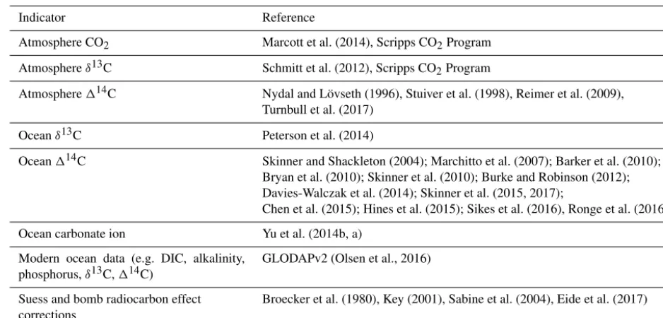
Table 2.Ocean and atmosphere data sources for the SCP-M modern carbon cycle calibration, projections and LGM–Holocene experiment.
Indicator Reference
Atmosphere CO2 Marcott et al. (2014), Scripps CO2Program
Atmosphereδ13C Schmitt et al. (2012), Scripps CO2Program
Atmosphere114C Nydal and Lövseth (1996), Stuiver et al. (1998), Reimer et al. (2009), Turnbull et al. (2017)
Oceanδ13C Peterson et al. (2014)
Ocean114C Skinner and Shackleton (2004); Marchitto et al. (2007); Barker et al. (2010); Bryan et al. (2010); Skinner et al. (2010); Burke and Robinson (2012); Davies-Walczak et al. (2014); Skinner et al. (2015, 2017);
Chen et al. (2015); Hines et al. (2015); Sikes et al. (2016), Ronge et al. (2016),
Ocean carbonate ion Yu et al. (2014b, a)
Modern ocean data (e.g. DIC, alkalinity, phosphorus,δ13C,114C)
GLODAPv2 (Olsen et al., 2016)
Suess and bomb radiocarbon effect corrections
Broecker et al. (1980), Key (2001), Sabine et al. (2004), Eide et al. (2017)
The late Holocene is chosen as the initial model calibration due to the absence of industrial-era CO2and bomb radiocarbon. Scripps CO2Program data originally sourced from http://scrippsco2.ucsd.edu (last access: 10 June 2018); data currently being transitioned to http://cdiac.ess-dive.lbl.gov (last access: 10 June 2018). The Peterson et al. (2014) database incorporates∼500core records across the LGM and late Holocene periods.
data accumulated over the period 1972–2013. We make ad-justments to the ocean concentrations of DIC,δ13C and114C for the effects of industrial emissions (the “Suess” effect) and bomb radiocarbon in the atmosphere using published esti-mates (Broecker et al., 1980; Key, 2001; Sabine et al., 2004; Eide et al., 2017). For example, Eide et al. (2017) establish a mathematical relationship between Suessδ13C and CFC-12 in the ocean, which we applied using GLODAPv2 CFC-12 data to correct the oceanδ13C data. We force the model with late Holocene average data for atmosphere CO2,δ13C and 114C (data sources in Table 2). The model’s starting param-eters are set from literature values (Table A1, Appendix), in-cluding the point estimates for ocean circulation and mixing fluxes from Talley (2013).
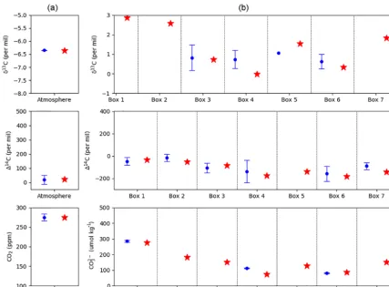
Using the Suess- and bomb-adjusted GLODAPv2 ocean dataset and late Holocene atmosphere data as the starting point, combined with the literature-determined parameter values, the model is allowed to run freely for 15 kyr in spin-up. This spin-up is ample time for model equilibration and to allow slower processes such as carbonate compensation to take effect. The resulting model equilibrium ocean and at-mosphere element concentrations from the spin-up are stored and then carried forward as the starting data for subsequent late Holocene simulations. Figure 3 shows the results of the model spin-up (red stars) compared with late Holocene atmo-sphere data and their standard error (blue dots and error bars) across the time period. We also show the model results com-pared with late Holocene ocean data from various sources (Table 2), which are averaged into the box model regions for comparison.
The late Holocene calibration convincingly satisfies the at-mospheric data values for CO2,δ13C and114C. Model re-sults are also in good agreement with the late Holocene ocean
114C, falling within error or very close for all boxes covered by data. The surface boxes (1, 2) are relatively enriched in
114C relative to deeper boxes, reflecting their proximity to the atmospheric source of14C, although the spread of values across the ocean boxes is narrow. The surface boxes (1, 2 and 7) intuitively display more enrichedδ13C than the intermedi-ate (3), deep (4) and abyssal (6) boxes, mainly due to the ef-fects of the biological pump. For most of the model’s boxes, the results fall within the standard error of the late Holocene
δ13C data. The Southern Ocean box (5) is an exception due to its extensive vertical coverage of 2500 m, incorporating the surface boundary with the atmosphere and the deep ocean, coupled with the sparseδ13C core data for the polar Southern Ocean (one data point, no error bars). SCP-M also exagger-ates the depletion inδ13C in the deep box (4) relative to the data observation.
Figure 3.SCP-M late-Holocene-calibrated model results using model input parameters from the literature (Table A1).(a)Model results for atmosphericδ13C,114C and CO2(red stars) plotted against late Holocene average data values (blue dots) with standard error bars.(b)The model results for oceanic δ13C,114C and the carbonate ion proxy (red stars) plotted against late Holocene average ocean data where available (blue dots). Data sources are shown in Table 2.
more carbon relative to alkalinity due to the remineralisation of organic matter, a pattern that SCP-M replicates.
3.2 Sensitivity tests
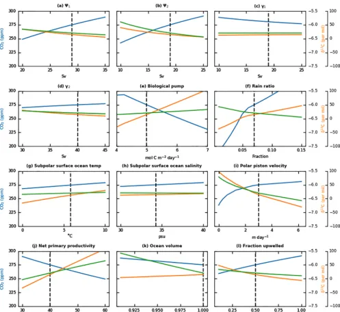
We undertook parameter sensitivity tests to understand changes in atmospheric CO2,114C andδ13C in SCP-M. This serves two purposes: (1) to understand the directional rela-tionship between the parameter values and these key model outputs, and evaluate whether they make sense, and (2) to in-form the LGM–Holocene model–data experiment in the fol-lowing section. For example, if the GOC parameter91 dis-plays a negative relationship with atmospheric CO2, it would make sense to probe parameter values lower than modern to replicate the lower atmospheric CO2in the LGM. We varied parameter values around their modern-day settings in 10 kyr model runs and plotted the output against atmospheric CO2, 114C andδ13C (Fig. 4).
For example, Fig. 4a–d shows sensitivity variations above and below the model’s modern values for ocean circulation and mixing parameters, sourced from Talley (2013) and Tog-gweiler (1999). Atmospheric CO2 is very sensitive to 91
and92but displays limited response toγ1andγ2 over the ranges analysed (Fig. 4a–d). Atmospheric114C andδ13C are negatively related to91and92. The slower ocean turnover leads to a reduced rate of upwelling and surface de-gassing of114C- andδ13C-depleted waters, causing higher values in the atmosphere. The effect of the mixing parameters on the atmosphere variables is muted because they have a limited impact on the upwelling regime for carbon, with any upward flux of carbon offset by a downward flux (mixing).
The soft tissue export flux parameter,Z, displays an in-verse relationship with CO2(Fig. 4e). A higher global value ofZdrives the removal of carbon from the surface ocean, and the resulting CO2flux into the ocean from the atmosphere de-creases CO2. LowerZ leads to increased atmospheric CO2. δ13C is particularly sensitive toZ, moving it well away from modern (and therefore Holocene and LGM) values from a minor perturbation. The rain ratio (Fig. 4f) increasespCO2in the surface ocean boxes, leading to de-gassing of CO2to the atmosphere, and therefore modestly decreasing atmospheric
Figure 4.Univariate parameter sensitivity tests around modern-day estimated values plotted for atmospheric CO2,114C andδ13C ver-sus(a)91,(b)92,(c)γ1,(d)γ2,(e)biological pump,(f)rain ratio,(g)subpolar surface box temperature,(h)subpolar surface box salinity, (i)polar box piston velocity,(j)net primary productivity,(k)ocean volume and(l)fraction of deep water upwelled into the subpolar surface box. We varied parameter input values as plotted on thexaxes and show model output for atmospheric CO2,114C andδ13C. Atmospheric CO2shows the greatest sensitivity to parameters associated with ocean circulation, biology and the terrestrial biosphere. Other parameters exert less influence on atmospheric CO2but are important for atmospheric carbon isotope values. Modern-day estimates used in SCP-M are shown with vertical black dotted lines in each subplot (sources in the text and Appendix Table A1).
Increasing surface ocean box temperature (Fig. 4g) in-creases atmospheric CO2, an intuitive outcome given that warmer water absorbs less CO2(Weiss, 1974), and SCP-M employs a temperature- and salinity-dependent CO2 solubil-ity function. Air–sea fractionation of δ13C also decreases with higher temperatures, leading to higher atmospheric
δ13C. According to Mook et al. (1974), air-to-sea fractiona-tion ofδ13C (making the atmosphere more depleted inδ13C)
As the polar box piston velocityP slows down (Fig. 4i), atmospheric CO2falls. At lower values ofP the polar box, a region of outgassing of CO2due to the upwelling of deep-sourced carbon-rich water in that part of the ocean, will ex-change CO2 with the atmosphere at a slower rate. The re-duced outgassing ofδ13C-depleted carbon to the atmosphere with a lowerP leads to higherδ13C values in the atmosphere. Atmospheric114C increases with a slowing ofP as the path-ways for it to invade the ocean from its atmospheric source are slower, and there is reduced outgassing of old, low114C waters.
Terrestrial biosphere NPP (Fig. 4j) is a sink of CO2and fractionates the ratios of the isotopes of carbon, leading to higher values for δ13C and, to a lesser extent,114C in the atmosphere. It is likely that NPP plays a feedback role and modulates CO2,δ13C and114C (Toggweiler, 2008). Varying the ocean surface area (Fig. 4k) has modest impacts on CO2 andδ13C, but a large impact on114C. Decreasing the ocean volume leads to a lower surface area for CO2and atmospher-ically produced radiocarbon to enter the ocean, causing them to increase in the atmosphere. We expect that changing the ocean surface area (from sea level), and therefore volume, leads to changes inpCO2on glacial–interglacial timescales. Increasing the fraction of deep water upwelled into the sub-polar box (Fig. 4l) intuitively raises CO2, but lowers δ13C and 114C, by upwelling carbon-rich and isotopically de-pleted water to the ocean surface boxes.
3.3 Modern carbon cycle simulation
Human fossil fuel and land use change emissions contributed
∼575 Gt carbon to the atmosphere between 1751 and 2010 (Boden et al., 2017; Houghton, 2010) and up until 2014 were growing at an accelerating rate. In response, the Earth’s car-bon cycle continually partitions carcar-bon between its compo-nent reservoirs, with positive and negative feedbacks. The net effect is a build-up of carbon in most reservoirs. Given the dominance of the anthropogenic emissions source in the modern global carbon cycle, a simulation model should be able to provide a plausible replication of its effects.
We modelled the effects of anthropogenic emissions and atmospheric nuclear bomb testing on the carbon reser-voirs and fluxes in SCP-M. The experiment forces the late Holocene–pre-industrial SCP-M equilibrium described in Sect. 3.1, with estimates of industrial fossil fuel and land use change CO2 emissions, sea surface temperature (SST) changes and atmospheric bomb 14C fluxes from historical data dating from 1751. For the future years to 2100, we force the model with the IPCC’s Representative Concentra-tion Pathway (RCP) CO2emissions and SST scenarios (Bo-den et al., 2017; Houghton, 2010; IPCC, 2013a). We compare the model results with atmospheric CO2,δ13C and114C his-torical data and published modelling results for future years from the CMIP5 project (https://cmip.llnl.gov/cmip5/, last access: 25 June 2018).
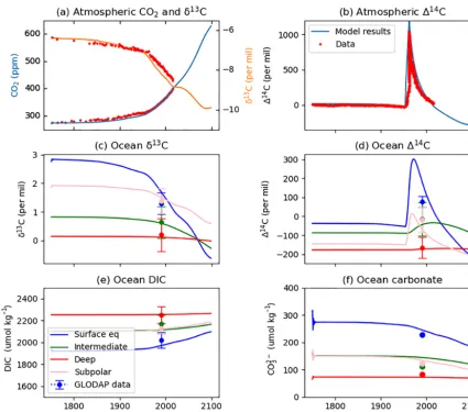
Figure 5 shows the modern carbon cycle simulation us-ing SCP-M compared with historical atmospheric data for CO2,δ13C and114C and GLODAPv2 ocean data (estimated data year 1990). Importantly, SCP-M provides an appropri-ate simulation of the carbon cycle response to human emis-sions inputs by replicating the atmospheric patterns for CO2, δ13C and114C preserved in data observations for the period 1751–2016 (a–b). The atmospheric CO2 andδ13C data are sourced from the Scripps CO2Program (originally sourced from http://scrippsco2.ucsd.edu, last access: 10 June 2018; data currently being transitioned to http://cdiac.ess-dive.lbl. gov, last access: 10 June 2018), and114C data are sourced from Nydal and Lövseth (1996), Stuiver et al. (1998), and Turnbull et al. (2017). A key feature of the historical data is the substantial increase in human emissions from circa 1950 onwards, which is accompanied by higher atmospheric CO2 and a steep drop inδ13C (Fig. 5a); this reflectsδ13C-depleted anthropogenic emissions. The effect of emissions on atmo-spheric114C (Fig. 5b) in the 20th century is largely over-printed by the influence of bomb radiocarbon. Emissions are seen as a slight downturn in the model and data114C in the immediate lead-up to the release of bomb radiocarbon into the atmosphere and the downward trend from∼2020 on-wards. The spike in114C during the period of bomb radio-carbon release lasts during the period 1954–1963 and then disperses as14C is absorbed by the ocean. The simulation shows that SCP-M agrees with the GLODAPv2 ocean data by 1990 (Fig. 5c–f), with most boxes falling within the stan-dard deviation of average data values, lending confidence to the model’s simulation of the redistribution of carbon.
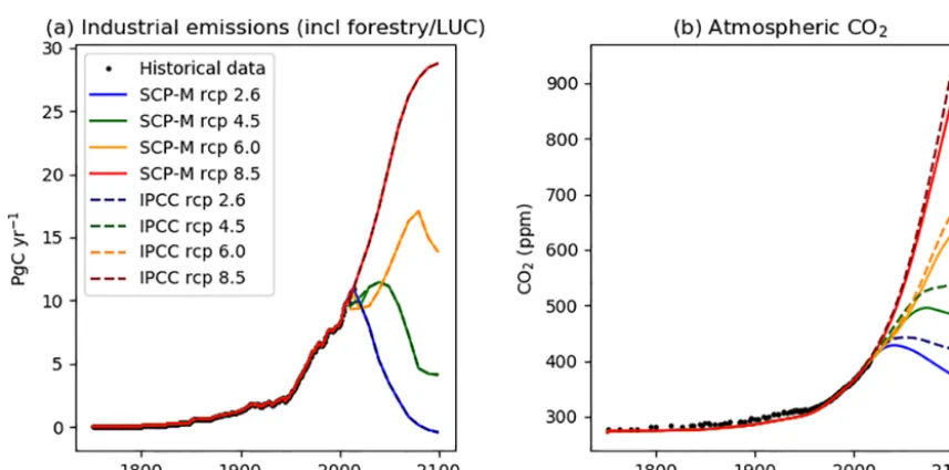
Figure 6 shows the emissions profile (a) and modelling re-sults for atmospheric CO2(b) over historical time and pro-jected forward to 2100 for the IPCC RCPs. The SCP-M out-put falls below the IPCC projections for atmospheric CO2in RCP2.6 and 4.5, but provides a close match with RCP6.0 and 8.5.
Figure 7a shows the annual uptake of CO2by the ocean, modelled with SCP-M. The model begins the period close to a steady state between the atmosphere and surface ocean
Figure 5.SCP-M modelling results compared with modern atmospheric and ocean GLODAPv2 data for(a)atmospheric CO2andδ13C, (b) atmospheric114C,(c)oceanδ13C,(d)114C,(e)DIC, and(f)the carbonate ion proxy. Projections beyond 2016 include the RCP6.0 emissions trajectory. In(a–b)we plot SCP-M model results for CO2,δ13C and114C (lines) for the period 1751–2100 against atmospheric data for CO2,δ13C and114C (red dots). The SCP-M model output closely resembles the atmospheric data record. The perturbation from industrial-era, isotopically depleted (δ13C) and dead (114C) CO2is clear, as is the impact of atmospheric nuclear tests on114C during 1954–1963. In the other rows we plot SCP-M model results (boxes as shown) versus GLODAPv2 data (dots and error bars, same colour as corresponding boxes). We assume an average data year of 1990 for the GLODAPv2 data accumulated over the period 1972–2013. For most of the SCP-M ocean boxes, the model results fall within or very close to error ranges of the GLODAPv2 data, despite large perturbations in the model and data from industrial-era emissions and bomb radiocarbon.
of cumulative uptake by the ocean by 2100 from 11 CMIP5 models, a closer range to the SCP-M outcomes.
Figure 8 shows the partitioning of anthropogenic CO2 emissions into the carbon cycle reservoirs in RCP6.0 by 2100, as simulated with SCP-M and compared with mod-elling results presented by the IPCC for the same scenario (IPCC, 2013b). By this time, the load of human emissions is roughly 45:55 split between the atmosphere and the com-bined terrestrial biosphere and ocean.
By 2100, in RCP6.0 the carbon cycle is substantially changed from the pre-industrial–late Holocene state. This is the result of the accumulation of hundreds of years of hu-man industrial CO2 emissions in the atmosphere and other
Figure 6.SCP-M RCP modelling results compared with IPCC emissions and CO2scenarios. Panel(a)shows the IPCC’s RCP emissions pathways out to 2100, which are inputted to SCP-M for the modern carbon cycle simulation. Panel(b)shows SCP-M model output for atmospheric CO2(firm lines) plotted against IPCC atmospheric CO2projections for the RCP pathways (dashed lines). The SCP-M output undershoots the IPCC projections for RCP2.6 and 4.5, but provides a close match with RCP6.0 and 8.5.
The terrestrial biosphere influx of carbon is dramatically in-creased by the carbon fertilisation effect, leading to a larger biomass stock, which in turn also causes more respiration – both inward and outward biosphere fluxes of CO2are there-fore greatly enhanced. The weathering of silicate rocks on the continents, a weak sink of carbon, also accelerates under the effects of burgeoning atmospheric CO2, transferring car-bon from the atmosphere to the ocean via rivers. The phys-ical fluxes of carbon within the ocean are only modestly af-fected, with the main exception being low-latitude thermo-cline mixing, which in RCP6.0 mixes a larger amount of carbon back into the surface ocean box from intermediate depths. The altered balance of DIC:alkalinity, particularly in the abyssal box, leads to a decrease in the carbonate ion concentration of abyssal waters late in the projection period, which in turn causes more dissolution of marine sediments. By 2100 this feedback brings more carbon back into the ocean, increased from 0.2 to 1.1 PgC yr−1, but also alkalin-ity (in a ratio of 2:1 to DIC), thereby lowering whole-ocean
pCO2 – a modest negative feedback. In summary, SCP-M provides an appropriate simulation of historical atmospheric CO2,δ13C and114C data when forced with anthropogenic CO2emissions data over the same period. For the forward-looking RCP emissions projections, SCP-M falls in the range of the CMIP5 models, although the oceanic carbon uptake is exaggerated for the RCP8.5 scenario. This result suggests that a more detailed experiment, for example with non-linear representation of the piston velocity with respect to atmo-spheric CO2or prescribed feedbacks from ocean circulation and biology (e.g. Meehl et al., 2007; IPCC, 2013a, b; Moore et al., 2018), might provide a closer fit to the CMIP5 models.
4 LGM–Holocene model–data experiment
4.1 Background
Togg-Figure 7.Panel(a)shows the annual uptake of CO2by the ocean in each of the RCPs over the period 1751–2100, modelled with SCP-M. By 2100, SCP-M estimates a range of 0–6 PgC yr−1across the RCPs as estimated by CMIP5 models, reproduced from Jones et al. (2013). Panel(b)shows the cumulative uptake of CO2by the ocean over the same period modelled with SCP-M and compared with CMIP5 models (Jones et al., 2013).
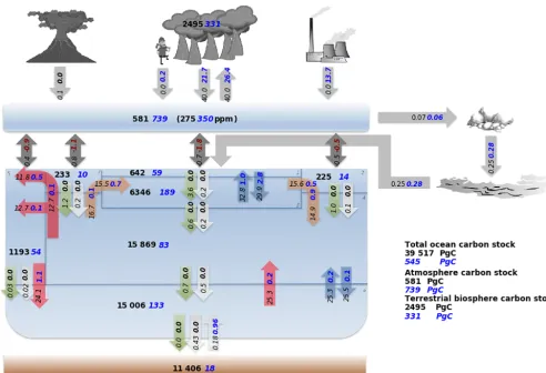
Figure 9.SCP-M-modelled pre-industrial carbon stocks and fluxes (in PgC in black text) compared with IPCC RCP6.0 emissions scenario by 2100 (shown as PgC changes with blue text for positive changes, red text for negative and black text for no change). Atmosphere, ocean and terrestrial biospheres take up the load of carbon from the industrial source. By 2100, carbon is fluxing into all ocean boxes, the terrestrial biosphere and continental sediment weathering–river fluxes. Pre-industrial outgassing of CO2in the Southern Ocean is reversed, and carbon is returned to the ocean via enhanced CaCO3dissolution. Box numbers on the diagram refer to ocean regions specified in Fig. 1. Negative fluxes on bidirectional air–sea exchange arrows are fluxes of CO2out of the atmosphere into the ocean.
weiler, 1984; Toggweiler and Sarmiento, 1985; Toggweiler, 1999; Curry and Oppo, 2005; Anderson et al., 2009; Ko-hfeld and Ridgewell, 2009; De Boer and Hogg, 2014; Men-viel et al., 2016; Muglia et al., 2018), sea-ice cover (Stephens and Keeling, 2000), whole-ocean chemistry (Broecker, 1982; Sigman et al., 2010), and composite hypotheses (Kohfeld and Ridgewell, 2009; Ferrari et al., 2014; Kohfeld and Chase, 2017). Other mechanisms proposed include ocean temper-ature, the terrestrial biosphere, ocean volume and shelf car-bonates (Opdyke and Walker, 1992; Trent-Staid and Prell, 2002; Ridgewell et al., 2003; Ciais et al., 2012; Annan and Hargreaves, 2013). Each hypothesis listed above is supported by site-specific tracer observations (e.g. marine carbonate cores), regional data aggregation and review, literature syn-thesis, or modelling. Within the spectrum of hypotheses, a simple explanation of a carbon cycle mechanism or mech-anisms remains elusive. Many of the early hypotheses were
presented as independent or even competing in causality for the interglacial CO2variation (Ferrari et al., 2014).
from the finding of Muglia et al. (2018), who specifically ex-amined the AMOC and Southern Ocean biological produc-tivity. They found that a weaker AMOC and stronger biolog-ical productivity could account for the LGM and Holocene
δ13C,114C and15N data. The GOC was not tested by Muglia et al. (2018). Kurahashi-Nakamura et al. (2017) contradicted both studies, diagnosing a more vigorous (but shallower) AMOC in the LGM, using a GCM with data assimilation of various proxies, notably only incorporating Atlantic data for the LGM.
4.2 Model–data experiments
We illustrate SCP-M’s capabilities by solving for the pa-rameter values of best fit with late Holocene and LGM ocean and atmosphere proxy data using a comprehensive model results–data optimisation. For this illustrative exam-ple, the atmosphere and ocean data are taken from published sources (Table 2), averaged for the LGM (∼18–24 ka) and late Holocene (6.0–0.2 ka) time periods and for box coor-dinates in SCP-M for the ocean data (depth and latitude). The mean and variance for each box are then calculated in SCP-M. First, we probe the potential for key model param-eters to drive Holocene–LGM changes in atmospheric car-bon variables to focus our experiment on these parameters. It is likely that the LGM-to-Holocene carbon cycle changes were dominated by the ocean (Sigman and Boyle, 2000; Kohfeld and Ridgewell, 2009), but were also accompanied by a range of physical changes in the atmosphere and ter-restrial biosphere that in aggregate could be material (e.g. Sigman and Boyle, 2000; Adkins et al., 2002; Kohfeld and Ridgewell, 2009; Ferrari et al., 2014). These changes include sea surface temperature, salinity, sea-ice cover, ocean vol-ume and atmospheric14C production rate. Estimates of av-erage sea surface temperature for the LGM generally fall in the range of 3–8◦C cooler than the present (Trent-Staid and Prell, 2002; Annan and Hargreaves, 2013). Adkins et al. (2002) estimated that ocean salinity was 1–2 psu higher in the LGM and sea levels were∼120 m lower (Adkins et al., 2002; Grant et al., 2014). Stephens and Keeling (2000) and Ferrari et al. (2014) highlighted the role of expanded sea-ice cover in the Southern Ocean during the LGM as a key part of the LGM CO2drawdown. Finally, Mariotti et al. (2013) es-timated that higher atmospheric radiocarbon production ac-counted for + ∼200‰ in atmospheric 114C in the LGM. Mariotti et al. (2013) simulated this variation in model ex-periments by increasing the radiocarbon production rate by a multiple of 1.15–1.30 (best guess 1.25) of the modern es-timate in order to recreate LGM114C values. Using these findings we define two background states for modelling pur-poses: a late Holocene state (Table A1 in the Appendix) and the LGM state (Table 3). Figure 10 shows the cumulative effect of these changes in SCP-M, within the late Holocene– LGM atmosphere 3-D CO2–δ13C–114C data space.
These changes are the first stage of a model adjustment to analyse the potential for ocean circulation and biologi-cal changes to deliver the LGM atmospheric CO2,δ13C and 114C values and transition the model output from the red cir-cle (late Holocene) to the black star (the LGM background settings), and then to the black circle (LGM). The decrease in ocean surface box temperatures leads to a drop in CO2 of∼20 ppm and a lightening ofδ13C by∼0.6 ‰ owing to the increased solubility of CO2 in colder water and the in-creasing fractionation ofδ13C with decreasing temperatures, which leaves more12C in the atmosphere. There is limited impact on114C. Increasing salinity slightly reverses these changes to CO2 andδ13C. Reducing sea surface area and volume slightly increases CO2 and increases 114C as the ocean’s capacity to take up these elements is reduced. Slow-ing down the piston velocity in the polar Southern Ocean box, as a proxy for increased sea-ice cover, slightly reduces CO2(reduced outgassing), increases114C (slower rate of in-vasion to the ocean) and increasesδ13C (reduced outgassing and sea-to-air fractionation ofδ13C). Finally, increasing the rate of atmospheric radiocarbon production forces a shift in
114C (horizontal shift in Fig. 10) towards LGM levels (black star and circle in Fig. 10). In aggregate, these changes lead to a fall in CO2of∼35 ppm, a fall inδ13C of∼ −0.5 ‰ and an increase in114C of∼300 ‰.
From the black star in Fig. 10, the “LGM state”, we perform a focussed sensitivity test on key hypothesised drivers of LGM–Holocene carbon cycle changes (Kohfeld and Ridgewell, 2009; Sigman et al., 2010). These are slower GOC (91), slower AMOC (92), reduced deep–abyssal ocean mixing (γ1) and a stronger biological pump (Z). The Z global biological production parameter, varied across 5– 10 mol C m−2yr−1(i.e. increased), can deliver the LGM CO
2 changes, but steersδ13C and114C away from their LGM values.γ1drives ancillary changes in all three variables, sug-gesting it is not the driver of the LGM atmospheric changes but may play a modulating role. Both91(3–29 Sv) and92 (3–19 Sv) experiments run very close to the LGM data values on their own, although neither can deliver a precise hit.
Using the literature-referenced Holocene and LGM back-ground parameter states, and informed by the sensitivity analysis in Fig. 10, we take advantage of SCP-M’s fast run time to perform thousands of multi-variant simulations over the free-floating91, 92, γ1 andZ parameter spaces using the SCP-M batch module. We then perform an optimisation routine against the data for each period to solve for values for
91,92,γ1andZ. The SCP-M batch module cycles through each set of parameter combinations, with each model simu-lation run for 10 000 years. Table 4 shows the experiment pa-rameter ranges for the late Holocene and LGM model–data experiments.
Table 3.Changes to ocean and atmosphere parameter settings in SCP-M to recreate the LGM background model state.
Indicator LGM change
Surface ocean box temperatures −5–6◦C (Trent-Staid and Prell, 2002; Annan and Hargreaves, 2013) Surface ocean box salinity +1.0 psu (Adkins et al., 2002)
Polar ocean box piston velocity ×0.3 (Stephens and Keeling, 2000; Ferrari et al., 2014) Ocean surface area and volume −3.0 % (Adkins et al., 2002; Grant et al., 2014) Atmosphere radiocarbon production ×1.25 (Mariotti et al., 2013)
As shown in the sensitivity tests in Fig. 4, some processes do not exert a strong influence on atmospheric CO2, but do modestly impact CO2 and strongly impactδ13Cand114C. Where these features are posited to vary around glacial cycles, we have incorporated them as a step change from late Holocene–modern estimates in our LGM experiment.
Figure 10.LGM state parameter adjustments. Using the posited LGM changes in environmental parameters in Table 3, we establish LGM foundations for exploring the impacts of varying large-scale ocean process parameters towards LGM atmospheric CO2–δ13C–114C data space. The red circle is our starting point for the late Holocene. From the LGM state foundation (black star), variation of global overturning circulation (91), Atlantic meridional overturning circulation (92) and the soft tissue biological pump (Z) drives atmospheric CO2,δ13C and 114C into the vicinity of their LGM data values (black circle). The biological pumpZcan effect the LGM CO2outcome, but steersδ13C away from the LGM value. Both91(3–29 Sv) and92(3–19 Sv) experiments run very close to the LGM data values on their own, although neither can deliver a precise hit.
for91and92(weaker ocean circulation) and higher values forZ(increased biological productivity) in the LGM experi-ment. Where the experiments resulted in a parameter output value at the limit of the input range, the range was widened and the experiment was repeated; 16 896 and 47 616 simula-tions were undertaken for the late Holocene and LGM exper-iments, respectively.
The SCP-M script harvests model output and performs a least-squares optimisation of the output against the LGM and late Holocene data for atmospheric CO2, atmospheric, and
ocean114C and δ13C, and also the oceanic carbonate ion proxy, to source the best-fit parameter values for91,92,γ1 andZ(or any parameter specified):
Optn=1=Min N
X
i,k=1 R
i,k−Di,k
σi,k
2
, (27)
where Optn=1represents the optimal value of parametersn,