Why Does Trend Growth Affect
Equilibrium Employment?
A New Explanation of an Old Puzzle
Michael W. L. Elsby
University of Edinburgh and NBER
Matthew D. Shapiro
University of Michigan and NBER
May 2, 2011
Abstract
That the employment rate appears to respond to changes in trend growth is an
enduring macroeconomic puzzle. This paper shows that, in the presence of a return
to experience, a slowdown in productivity growth raises reservation wages, thereby
lowering aggregate employment.
The paper develops new evidence that shows this mechanism is important for
ex-plaining the growth-employment puzzle. The combined e¤ects of changes in aggregate
wage growth and returns to experience account for all the increase from 1968 to 2006
in nonemployment among low-skilled men and for approximately half the increase in
nonemployment among all men.
I
Introduction
Explaining the variation in rates of employment over time has been a central question for labor and macroeconomics and for public policy for several decades. The sudden and sus-tained increase in nonemployment beginning in the early 1970s occurred at the same time as the rate of growth of productivity and wages slowed. From 1970 to 1980, the nonemployment rate of prime age adult males in the United States rose from 6 percent to 12 percent (see Figure 1A). These trends were associated with dramatic declines in labor market attachment among the low-skilled. For high school dropouts, rates of nonemployment rose from 10 per-cent to 23 perper-cent over the same period (Figure 1B). The 1970s also saw a dramatic slowing of the rate of productivity and wage growth. Trend growth in wages for all adult males fell 5 percentage points over the 1970s (Figure 2). Economists have long been tempted to relate the decline in economy-wide wage growth associated with the productivity slowdown of the 1970s to the persistent deterioration in equilibrium employment beginning in the early to mid-1970s.1
Super…cially, the case for a link between productivity growth and employment rates appears simple: Should it be surprising that employment declines when the returns to work have fallen? The theoretical link between productivity growth and equilibrium employment, however, has proved elusive. In traditional models of the aggregate labor market (Layard, Nickell and Jackman, 1991), changes in trend rates of growth of productivity and wages do not a¤ect the steady-state rate of employment. That is, changes in productivity growth a¤ect equally the returns to work and the returns to not working, as any violation of this relation will cause an economy to converge either to full employment or zero employment in the long run. Indeed, in his survey of traditional models of employment determination, Blanchard (2007) concludes that they “deliver, to a …rst order, long run neutrality of unemployment to productivity growth.” Shimer (2010) demonstrates that the same neutrality result arises in a balanced-growth version of the Mortensen and Pissarides (1994) model. While existing theories have clearer implications for the short to medium run link between productivity growth and the rate of employment, the understanding of the link between them in the long run is weaker. To quote Blanchard (2007, p.416), “The truth is we do not know. And this is a serious hole in knowledge.”
Existing literature has attempted to break this employment/growth neutrality result. Theoretical work on unemployment in labor markets with frictions has identi…ed two channels through which growth can a¤ect unemployment in the long run. If technological change
1A prominent early example is Bruno and Sachs (1985). More recently, see Staiger, Stock, and Watson
is embodied in new jobs, a process of creative destruction arises whereby old jobs must be destroyed to update to the technological frontier (Aghion and Howitt, 1994). In this environment, faster growth implies higher rates of obsolescence, increased job destruction and increased unemployment, in contrast to the trends observed in the data. If new technologies are incorporated into all jobs, however, a capitalization e¤ect can occur: If the costs of job creation are borne upfront, higher expected productivity growth causes future pro…ts to be discounted at a lower rate, stimulating …rms’ demand for labor through job creation, and reducing unemployment (Mortensen and Pissarides, 1998; Pissarides and Vallanti, 2007).
This paper identi…es a novel and complementary explanation for the longstanding puzzle of providing a theoretical explanation for the observed low-frequency comovement of pro-ductivity growth and the employment rate. Our explanation of the puzzle is motivated by an additional salient feature of the data: that the decline in male employment rates was accompanied by sustained declines in labor force attachment. Accordingly, our explanation highlights the role of wage growth in the decision of workers to supply labor.
We begin by showing that Blanchard’s neutrality puzzle, which refers to the unemploy-ment margin, applies with the same force to the labor supply margin. Absent the e¤ects we emphasize, standard models of the work/nonwork decision imply that labor supply is unaf-fected by changes in trend productivity growth. We show that this result is overturned once one recognizes that workers face substantial returns to labor market experience. Since Weiss (1972), it has been well-understood that the joint processes of the accumulation of labor market experience and the decision to supply labor are naturally intertwined. In order to accumulate experience, an individual must work. Consequently, changes in the experience-earnings pro…le that workers face a¤ect the decision of a marginal worker to seek lifetime employment.
grouping together nonparticipation and unemployment. This choice is informed by the analy-sis of Juhn, Murphy and Topel (1991, 2002). While a clear distinction between unemploy-ment and nonparticipation may exist over the business cycle, they argue that the boundary between these two states is blurred at low frequencies. In their words, “[t]he composition of unemployment has shifted toward less skilled workers, who su¤er comparatively long spells of joblessness and whose rewards from work have fallen sharply. In both these respects, they resemble the growing class of men who have simply withdrawn from the labor market” (1991, p. 125). Viewed from this perspective, the model suggests that the combined e¤ects of changes in aggregate wage growth and returns to experience can account for all of the increase from 1968 to 2006 in nonemployment among low-skilled men, and around half of the increase in nonemployment among all men.
This view is not the only interpretation of the model, however. The second perspec-tive we consider is to align the labor supply margin that we model with the participation decision, rather than with nonemployment, implicitly grouping together employment and unemployment. Thus, we also examine the extent to which our explanation can account for secular trends in nonparticipation. Rates of nonparticipation among prime-age men in the United States rose profoundly from 4 percent in the late 1960s to 9 percent in the early 2000s (Figure 1C). Mirroring the skill pro…le of nonemployment shown in Figure 1B, the process of detachment from the labor market was concentrated among the low skilled, with high school dropouts facing rises in nonparticipation rates from 5 percent to 20 percent over the same period (Figure 1D). Reassuringly, the model also provides a good account of these trends in male labor force participation, over predicting slightly the rise in trend nonpar-ticipation among low-skilled workers, and accounting for the majority of the secular rise in aggregate male nonparticipation since the 1960s. Hence, our novel channel for relating pro-ductivity growth to the employment rate …nds empirical support whether viewed through the nonparticipation or nonemployment data.
The plan of the remainder of the paper is as follows.
In Section II, we present a very simple model of labor supply in the presence of a return to experience and aggregate wage growth in order to provide the basic qualitative intuition for the e¤ects we emphasize. This theory demonstrates transparently and intuitively how the returns to experience and the aggregate rate of wage growth interact to explain the correlation of the level of the employment rate and the rate of growth of productivity and wages.
growth on labor supply, and that reductions in job-…nding prospects discourage labor supply. Quantitively, however, we …nd that the magnitude of these e¤ects is likely to be modest.
In Section III, we then present empirical results that con…rm the substantial changes in aggregate wage growth and the return to experience among low-skilled, marginal workers. This section uses Decennial Census and Current Population Survey (CPS) data to study wage growth and the returns to experience for male workers by level of educational attainment. We …nd signi…cant changes in aggregate wage growth and the return to experience that, when combined with our theoretical analysis, help explain the productivity/employment puzzle. A novel empirical …nding is that the lowest skilled workers have experienced declines in the return to experience. Previous work …nds that the return to experience has generally increased. Our empirical work supports this …nding, but shows how these increases in the return to experience are not shared by the least-skilled workers. This …nding is pivotal for our analysis since these low-skilled workers are precisely the population on the margin for the work/not-work decision.
In Section IV, we extend the simple model of Section II to account for …nite worker lifetimes, as well as nonlinear experience-earnings pro…les. Using this generalized model, we then draw out the quantitative implications of the observed changes in wage growth documented in Section III for trends in male nonemployment and nonparticipation.
In Section V we discuss how this paper relates to the literature. In Section VI, we o¤er conclusions and discuss directions for future work.
II
The Productivity Growth/Employment Interaction:
Basic Model
We …rst present a simple model that delivers our basic insights on the interaction of aggregate wage growth and the return to labor market experience, and its role in the determination of incentives for lifetime employment. Consider a simple environment in which there are two employment states, employment and nonemployment, and workers choose whether they want to supply their labor or not. Note that the phenomenon we are aiming to model is the life-long choice that a worker makes to be committed to the labor market and therefore accrue the returns to experience. Consequently, we initially abstract from frictional episodes of unemployment between jobs.
an in…nitely lived workeriwho must make a once-and-for-all decision at the start of his (non) working life between working forever and not working forever. If he works, he accumulates a year of labor market experience xfor every year he works, and faces a wage pro…le wi(x; t). Assume that there is a return to experience gx, and aggregate wage growth gw, such that
lnwi(x; t) = lnwi(0;0) +gxx+gwt: (1)
It is straightforward to derive equation (1) as the labor demand equation implied by a constant returns to scale production technology with fully ‡exible inputs, in which a worker with experiencexaccounts foregxx e¢ ciency units of labor, and labor augmenting technical progress occurs at rate gw over time (see Appendix A for a derivation). If the individual decides not to work, he does not accumulate experience, and he receives a payo¤ from nonemployment equal to bi(t). Assume that the latter grows over time at rategb.2
In this simple environment, all the worker need do is choose the option that delivers the highest present value of lifetime earnings. In particular, if the discount rate is equal tor, it is straightforward to show that a newborn potential worker at time t will decide to work if his o¤ered wage, wi(0; t) exceeds a reservation wage equal to
wi(0; t) wRi(t) = bi(t), where
r gw gx
r gb
: (2)
This simple formulation for the reservation wage relies on an in…nite horizon speci…cation and an assumption of geometric growth in this simple model. In Section IV below, we present a more general model that preserves the intuition of this formulation for the reservation wage while taking into account a more realistic speci…cation of the trajectory of wages.
A
Wage Growth and Steady-State Employment
A number of insights follow from the simple observation in equation (2). First note that, while the reservation wage grows over time at the same rate as the payo¤ from nonemployment,gb, the wage of a newborn worker, w(0; t), grows at the rate of aggregate wage growth, gw. To see the signi…cance of this, imagine an economy populated by workers facing di¤erent wage pro…les,wi(x; t) =!iw(x; t), and di¤erent payo¤s from nonemployment, bi(t) = ib(t), but
2In this context, the ‡ow payo¤ from nonemployment b must include much more that unemployment
who otherwise face the same labor supply problem. The variables !i and i thus represent heterogeneity in skill and the payo¤ from nonemployment respectively. It follows that the steady-state employment rate in this economy will be given by
L = Pr [wi(0; t) bi(t)] = 1 ( ); (3)
where ( )is the c.d.f. of the ratio !i= i, and b(t)=w(0; t) is the replacement rate for newborn workers.
For employment to be in steady state, the replacement rate must be stationary. The replacement rate will be stationary only if the growth rate of the payo¤ from nonemployment is equal to the rate of aggregate wage growth, gb =gw in steady state. To see why, imagine for example thatgb > gw. In this case, the employment rate will converge to zero over time as the payo¤ from nonemployment increasingly dominates the payo¤ from work. A symmetric logic holds for the case where gb < gw. Imposing the restriction required for a steady state to exist, gb =gw, implies that the reservation wage may be rewritten as
wRi(t) = bi(t), where 1
gx
r gw
: (4)
Note that the constraintgw =gb is not special to our formulation. Any model with a steady state will have to impose it.
Together, equations (3) and (4) characterize the determinants of incentives to work in this simple environment. We observe that changes in employment are driven by changes in either or . The e¤ects of changes in the replacement rate are simple and well-understood: A higher replacement rate renders nonemployment more attractive and reduces steady state labor supply. This e¤ect is a very conventional long run property of models of equilibrium employment (see Blanchard, 2000; Layard, Nickell and Jackman, 1991, among others). The determinants of the variable are less common in the literature— the return to labor market experience,gx, the rate of aggregate wage growth,gw, and their interaction. We now explore these e¤ects in more detail.
Consider …rst the e¤ects of the return to experience. Note from equation (4) that a positive return to experience, gx > 0, drives a worker’s reservation wage below his ‡ow payo¤ from nonemployment. The reason is simple. If workers anticipate positive returns to experience, they will forgo earnings in the short run in order to reap the returns to experience in the long run. This point has long been noted since Weiss (1972), and more recently by Imai and Keane (2004), but has been largely neglected in macroeconomic models where wage growth is linked only to the level of productivity and not to labor market experience.3
A corollary of this observation is that increases in the return to experience will reduce reservation wages even further below the ‡ow payo¤ from nonemployment, and therefore will lead to increased employment rates. The reason is that increases in the return to experience raise the present discounted value of earnings from working relative to not working.
The key implication of (4) that underlies our account for the comovement between pro-ductivity growth and employment are the e¤ects of a change in the rate of aggregate wage growth, gw. Equation (4) reveals that there is an interaction between gx and gw: When the return to experience is positive, increases in the rate of aggregate wage growth lead to reductions in reservation wages, thereby raising aggregate employment. The simple reason is that greater aggregate wage growth interacts with the return to experience by compounding the rate of wage growth relative to the growth of the payo¤ from nonemployment. Aggregate wage growth acts like compound interest on the return to experience.4 It is important to note that the latter e¤ect of aggregate wage growth on incentives to supply labor is absent in traditional models of aggregate employment determination which abstract from returns to experience and implicitly set gx = 0. Highighting how a positive return to experience creates an e¤ect of the trend rate of growth on employment is a central contribution of this paper.
The perceptive reader will observe that the e¤ect of aggregate wage growth in our model is driven by the speci…cation that experience is multiplicative, not additive, in determining wages, i.e. that the Mincerian wage equation be speci…ed in logarithms rather than in levels. The speci…cation that experience and productivity are multiplicative is, however, much deeper than a functional form restriction. If the returns to experience were additive in wages, i.e., a …xed amount rather than …xed percentage, then the returns to experience would become vanishingly small over time if there is a positive trend to productivity. So a linearly additive speci…cation for experience is equivalent to assuming no steady-state return to experience whatsoever.
Ben-Porath (1967) has highlighted the implications of the joint determination of human capital accumulation and labor supply for the life cycle pro…les of earnings and hours worked (Blinder and Weiss, 1976; Heckman, 1976; Ryder, Sta¤ord and Stephan, 1976), education choice (Willis and Rosen, 1979) and the estimation of preference and technology parameters (Shaw, 1989; Lee, 2008). See Weiss and Rubinstein (2006) for a survey. Perhaps most related to the present paper is the analysis of Olivetti (2006), who emphasizes the role of changes in returns to experience among women since the 1970s. In contrast to our analysis of low-skilled males, she …nds evidence of steepening experience-earnings pro…les among women, and identi…es it as a key driving force for increased female labor force participation since the 1970s.
4The mechanism for the e¤ect of g
w on employment incentives, though simple, can appear subtle. A
B
Where Shocks Hit Hardest: The Importance of Marginal
Work-ers
The simple model of this section adds two novel determinants of variation in the aggregate employment rate: the return to experience and the rate of aggregate wage growth. A more precise expression for the e¤ects of changes ingw andgx on steady state employment can be obtained from logarithmic di¤erentiation of (3) to obtain,
lnL = " ln ; (5)
where " is the steady state elasticity of labor supply with respect to the wage,
" =
0( )
1 ( ): (6)
Note that " is the elasticity of labor supply on the extensive margin, i.e. the employment vs. nonemployment margin. Consequently, it measures the elasticity of the inverse c.d.f. of reservation wages in the economy.5
Thus, we see that the employment e¤ects of changes in the rates of aggregate wage growth and the return to experience are increasing in the size of the wage-elasticity of aggregate labor supply, ". The intuition for this result is simple. A small value of " implies that there are little incentive e¤ects of wages on workers’ choice to supply labor. This in turn extinguishes the labor supply e¤ects of wage growth which rely on the notion that wages incentivize labor supply.
The employment elasticity " will be particularly large for workers who are low-skilled. To see this, note that we can write the steady-state employment rate among workers of a given skill ! as
L (!) = 1 ( =!); (7) where ( ) is the c.d.f. of the inverse of workers’ idiosyncratic payo¤s from not working,
1= i. It follows that the wage elasticity of the employment rate for workers of skill! is equal to
"(!) =
!
0( =!)
1 ( =!): (8)
A su¢ cient condition for this elasticity to decline with skill, !, is that the modal worker
5Focusing on the extensive margin of labor supply abstracts from the possibilities that, facing lower
of that skill is employed.6 Thus, the model predicts that low-skilled workers respond to changes in the rate of aggregate productivity growth and the return to experience to a greater extent. The simple reason is that low-skilled workers are more likely to be on the margin of the employment decision than high-skilled workers, and therefore are more responsive to changes in the incentives to work.
This prediction of the model formalizes the intuition underlying the empirical analysis of Juhn, Murphy, and Topel (1991, 2002). They show that much of the increase in joblessness in the United States from the 1970s onward is concentrated among low-skilled workers, an observation that is replicated in Figure 1B. In addition, they provide estimates of the elasticity of labor supply by skill group (see Table 9 of their 1991 article and Table 10 of their 2002 article) that con…rm that low-skilled labor supply is much more elastic than for higher skilled workers. Both of these results are consistent with the formal implications of our model. We will see later in Section IV that the tight correspondence between our theoretical model and the empirical results of Juhn, Murphy, and Topel will enable to us to interpret and quantify the implications of our model for observed trends in joblessness in the United States over time.
C
Interactions with Labor Market Frictions
Thus far, our analysis has demonstrated the important role of wage growth in shaping reservation wages in a model in which individuals face no frictions to obtaining work. A natural question is whether the existence of labor market frictions may interact with wage growth in determining incentives to supply labor. One of the determinants of the decision to seek work might be the di¢ culty of obtaining work itself.
To explore this possibility, in this subsection we extend our basic model to incorporate such frictions. Speci…cally, if employed workers lose their job at rate s, and new job o¤ers arrive at rate f, we show in the Appendix that the reservation wage mirrors equation (4), except that the coe¢ cient is modi…ed slightly:
wRi(t) = ~bi(t), where ~ 1
gx
r gw
r+f gw
r+s+f gw
: (9)
This result motivates a number of observations. First, the addition of frictions shades down the e¤ects of wage growth by a factor r+f gw
r+s+f gw <1. Intuitively, episodes of frictional unemployment impede the accumulation of labor market experience for an individual who
6To see this, note that since =! is declining in !, the elasticity of aggregate labor supply for workers
supplies his labor. Second, consistent with the intuition that motivated this extension, reductions in the job-…nding rate lower the factor r+f gw
r+s+f gw, raising reservation wages, and disincentivising labor supply.
In addition to these qualitative e¤ects, however, equation (9) also provides guidance on the likely quantitative magnitude of these e¤ects. Speci…cally, for empirically-plausible values of the ‡ow transition ratess andf, an excellent approximation to the additional term
r+f gw
r+s+f gw is simply f s+f.
7 A useful interpretation of the latter is that it is equal to one minus
the steady-state rate of frictional unemployment. Thus, a very good intuitive rule of thumb is to imagine that an individual who supplies his labor will be employed a fraction s+ff of his working life, and so will accrue the same fraction of the total possible returns to experience. By the same token, this interpretation clari…es that any interactions between the e¤ects we emphasize and labor market frictions are likely to be modest in magnitude. The reason is that empirically-plausible values for the rate of unemployment imply values of s+ff that are very close to one. This suggests that the e¤ects of wage growth on reservation wages implied by the frictionless model underlying equation (4) are a very good guide to the same e¤ects in the presence of frictions in equation (9). This point does not preclude that changes in wage growth may a¤ect rates of job-…nding, and thereby rates of unemployment, for example via the capitalization e¤ects emphasized by Mortensen and Pissarides (1998) and Pissarides and Vallanti (2007). We return to this point in Section V.8
D
Summary of Qualitative Predictions
This section has used a very simple model to elucidate the e¤ects of wage growth on aggregate employment in an environment that incorporates a return to labor market experience. It has established the following qualitative predictions: First, increases in the rate of return to experience reduce reservation wages and stimulate aggregate employment by increasing the present discounted value of working over not working. Second, if there is a positive return to experience, increases in the rate of aggregate wage growth will also reduce reservation wages and raise aggregate employment. And …nally, the employment e¤ects of wage growth, of the return to experience, and of the interaction of wage growth and the return to experience will be greatest among low-skilled workers who are the most marginal to the employment
7For example, estimates for prime-age males reported by Fujita and Ramey (2006) suggest job-…nding
rates of approximately 0.33 and job-loss rates of approximately 0.015 on a monthly basis. These imply annual job-…nding and job-loss hazards of approximately 4 and 0.18 respectively, dwar…ng analogous values forrandgw.
8Our approach in this subsection mirrors a recent literature that has sought to incorporate both
decision. The evidence discussed in the next section bears directly on these e¤ects and how they might inform the growth rate/employment puzzle.
III
Evidence
In this section we take on the task of documenting evidence on changes in aggregate wage growth and in the returns to experience by skill for workers in the United States over time. In Section IV, we use this evidence, together with a generalization of the model of Section II, to simulate the e¤ects on employment rates of changes in the return to experience and its interaction with real wage growth.
A
Changes in Aggregate Wage Growth by Skill
To measure changes in the rate of aggregate wage growth we use March CPS microdata for the period 1967 to 2006. We restrict our samples along several dimensions. First, we concentrate on outcomes for white men since labor force participation issues for non-whites and women are signi…cantly more complicated (Smith and Welch, 1989; Welch, 1990; Blau, 1998). In particular, we restrict the samples to non-immigrant white males aged 16 to 64. Mirroring Juhn, Murphy and Topel’s (1991, 2002) in‡uential analyses of wages and employment by skill in the United States, we additionally focus on respondents with fewer than 30 years of potential experience who report that they were out of school for the entire year and are not self-employed. Wages are measured by dividing annual wages and salary by annual hours worked. As our theory makes clear, we are especially interested in changes in wage growth for marginal workers who are relatively low in the skill distribution. We use educational attainment as a proxy measure of skill. We distinguish among high school dropouts (9 to 11 years of education), high school graduates (12 years), those with some college education (13 to 15 years) and those with a college or higher degree (16+ years).9 Finally, to ensure that measured changes in aggregate wage growth are not driven by changes in the experience composition of our samples over time, we compute average wage growth from the distribution of wages reweighted to hold constant the distribution of experience using the method of DiNardo, Fortin and Lemieux (1996).
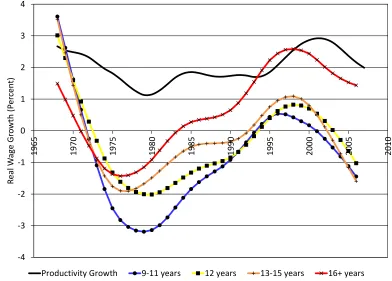
Figure 2 plots trend hourly wage growth by education from 1968 through to 2006 based on these CPS samples. Speci…cally, this takes estimates of real hourly wages by education, computes implied annual wage growth by education, and reports the HP …ltered series.
9Juhn, Murphy and Topel (1991, 2002) measure skill by percentiles of the wage distribution, rather than
This exercise reveals a clear picture of aggregate wage growth in recent decades. For all educational groups, aggregate wage growth fell in 1970s, rebounded in the 1980s and 1990s, and has fallen o¤ again in recent years. In addition, we observe that trend wage growth declined more acutely among low-skilled workers in the 1970s. Among high school dropouts, wage growth declined secularly in the 1970s from around 3 percent per year to trend real
wagedeclines of approximately 3 percent in late 1970s and early 1980s. In contrast, real wage
growth among college educated workers declined more slowly in the 1970s, and rebounded more robustly in the 1990s.10
These observations echo well-documented facts on aggregate growth, as well as wages by skill. The secular decline and subsequent rebound in aggregate wage growth over time mirrors the productivity slowdown of the 1970s as well as the so-called “productivity miracle” of the 1990s in the United States. Figure 2 overlays the trend productivity growth rate over the same period to emphasize these trends. Likewise, the observation that wage growth declined more sharply among the low-skilled in the late 1970s and 1980s is consistent with the widely documented increase in wage inequality that emerged over that period.
B
Changes in the Experience-Earnings Pro…le by Skill
To measure changes in the experience-earnings pro…le over time, we employ data taken from the decennial Censuses from 1960 to 2000, and the American Community Surveys from 2001 to 2007 for the United States.11 Earnings are measured by the annual wage and salary income of respondents. Mirroring our analysis of aggregate wage growth, we again proxy skill using discrete education categories: high school dropouts (9 to 11 years), high school graduates (12 years), some college (13 to 15 years), and college degree or higher (16+ years). Experience is measured by potential experience, i.e. age minus years of education minus six. We focus on the return to experience among full-time, full-year workers, de…ned as those who work 35 hours or more per week, and who are employed for 50 or more weeks per year. We do this for a number of reasons. By focusing on such workers, we can be more con…dent that respondents have left full-time education when we observe their earnings.
10A potentially important confound to the trends in Figure 2 is the growth of non–wage compensation
(such as health insurance, pensions and paid leave) that emerged over the period. It is di¢ cult to get an accurate sense of this from the data sources we use. However, using the microdata underlying the Employment Cost Index, Pierce (2001) shows that wage growth understated compensation growth among high–skilled workers in the 1980s, but that it overstated compensation growth among the low–skilled in the 1990s. Hence, for total compensation the relative growth rate in wages for low-skilled workers is likely to be even less favorable than shown in Figure 2.
11Our Census samples are taken from the public use 1% sample for 1960, 2% sample for 1970, and 5%
Moreover, the observed pro…les are more likely to re‡ect variation in wages rather than hours or weeks worked. Finally, the fact that we are able to measure only potential experience raises a concern that a changing relationship between potential and actual experience could confound observed changes in experience-earnings pro…les. By concentrating on full-time, full-year workers, such a confound is minimized.
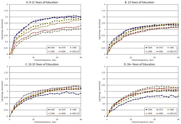
Figure 3 plots average log earnings as a function of potential experience by education group, normalized to the mean log earnings of workers entering the labor market. Log earnings are normalized to equal zero at zero experience to abstract from the signi…cant di¤erences in levels of earnings across education groups and of aggregate wages across time. These levels shifts in wages do not a¤ect equilibrium employment in our model. Within each panel, the lines correspond to the experience-earnings pro…les for di¤erent Census years for a given education group.12 Figure 3A displays the experience-earnings pro…le for high school dropouts (9-11 years of education) over time. Note that outcomes for these lower-skilled workers are of particular interest for our purposes because they are more likely to be marginal to the employment decision. Figure 3A tells a striking story. The experience-earnings pro…le among high school dropouts ‡attened dramatically after 1970. At …ve to ten years of potential experience, earnings are around 50 log points lower in the later period compared to the earlier period. In addition, the gap in the experience-earnings pro…le persists at higher levels of experience.
Figure 3B plots the experience pro…le for high school graduates. This reveals a mild drop in mid-career earnings between 1970 and 1990, with a more substantial drop in the experience-earnings pro…le between 1990 and 2000. In comparison to the outcomes for high school dropouts, the changes are relatively modest.13
As emphasized above, workers with schooling beyond high school are unlikely to be at the point in the skill distribution where employment is a marginal decision, so that patterns in experience-pro…les among these groups are less relevant to employment rates. By way of comparison, however, we include results in Figures 3C and 3D for workers with some college
12Prior to 1980, Census data record only hours last week, and after 1990 only usual hours of work. Reacting
to this, we impose the full-time restriction for the 1960 to 1990 pro…les based on hours last week. After 2000, we compute the di¤erence in the experience–earnings pro…le generated by implementing the full-time restriction using these alternative hours measures in 1990, when both measures are available. We then apply that di¤erence to impute the experience–earnings pro…les from 2000 on.
13For high school graduates and college educated workers, a number of studies in the empirical literature
education and a college degree or higher respectively. For these higher skilled workers, an opposite trend can be discerned, especially for college educated workers, with experience-earnings pro…les steepening over time.
A number of questions arise in the light of the substantial decline in the experience-earnings pro…le for high school dropouts in Figure 3A. First, in Appendix B, we consider the robustness of the result to a range of possibilities, including: a widening gap between potential and actual experience driven by the increases in joblessness documented in Figure 1; selection associated with the possibility of high school dropouts becoming less-skilled over time; and consistency with alternative measures of the experience premium. On all these dimensions, we …nd that the central message that the experience-earnings pro…le for high school dropouts has ‡attened substantially remains robust.
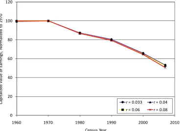
Second, given the robustness of this result, one might ask how big a reduction this is. A natural way to quantify the decline is to compute the capitalized value of the experience-earnings pro…les illustrated in Figure 3A. Figure 4 performs this exercise. It plots the capitalized value of the experience-earnings pro…les in Figure 3A, normalized to equal 100 in 1970, for a range of values for the discount rate. A clear picture emerges: Regardless of the discount rate, the value of the experience-earnings pro…le for high school dropouts declined by almost 50 percent between 1970 and 2007, a substantial reduction.
C
Synthetic vs. Actual Cohorts
The preceding results report cross-sectional experience-earnings pro…les at given points in time. For the purposes of our analysis of the likely employment e¤ects of any changes in these pro…les, we would like to obtain information on workers’ expectations of their likely experience pro…le at the time that they are making their labor supply decisions. It is likely that these cross-sectional pro…les are informative to some degree on these expectations— for instance, if workers have static expectations or changes are permanent, so that static expectations are rational.
An alternative way of slicing the data, however, would be to plot the realized experience-earnings pro…les of individual cohorts. This alternative approach would be consistent with workers’expectations if they were endowed with perfect foresight. The truth, of course, is likely to lie somewhere between these two extremes, so it is natural to check whether the basic message of the data changes by shifting perspective in this way.
only at a decadal frequency, we plot earnings for members of these cohorts every 10 years.14 For high school dropouts, while the cohort pro…les in Figure 5A are noticeably ‡atter after ten years of experience, the trends across cohorts tell exactly the same story as the cross-sectional picture in Figure 3A. Wage growth declines for each consecutive cohort entering the labor market after 1960, and the declines are of similar magnitude as those indicated by the cross-sectional pro…les in Figure 3A. These cohort-based pro…les mirror the …ndings of Kambourov and Manovskii (2009) using CPS and PSID data. The pro…les for high school graduates, and those with college education in Figures 5B, 5C and 5D also echo the patterns observed in their cross-sectional counterparts in Figure 3. Most noticeably, it is again possible to discern a steepening of experience-earnings pro…le among younger cohorts of college graduates. It is reassuring that these two di¤erent slices of the data have similar implications with respect to the changes in returns to experience over time.
IV
Quantitative Implications
To what the extent do the changes in aggregate wage growth and experience-earnings pro…les documented in Section III account for changes in the rate of nonemployment documented in Figure 1? In this section, we extend the simple model of Section II. The extended model retains the transparent qualitative predictions of the simple model while adding enough generality to allow for analysis based on the earnings pro…les quanti…ed in Section III.
A
A More General Model
The model of the Section II is simpli…ed in a number of respects. In this section we relax some of these simplifying assumptions. First, we allow for …nite worker lifetimes. This enables discussion of the di¤erential e¤ects of changes in wage growth across di¤erent cohorts of workers in a natural way. Second, we allow the return to experience to be nonlinear to allow for the concavity of the experience-log earnings pro…le observed in Figures 3 and 5. This allows us to match the experience-earnings pro…le in the model with that observed in the data. Third, we allow workers to choose whether to work or not at each point in their lives, thereby relaxing the once-and-for-all labor supply decision of Section II. Extending the model in this manner allows us to draw out the dynamic e¤ects of changes in rates of wage growth on employment in and out of steady state. Though more realistic, we will see that these changes do not change the basic qualitative message of the simple model of Section II.
14Additionally, we impute data points for 2010 under the assumption that the experience–earnings pro…le
Consider a worker entering the labor market at time s with a working life of length T. At each point in time the individual chooses whether he wants to work (h= 1) or not work (h = 0). As in the model of Section II, for every year he works, he accumulates a year of labor market experience,x; he does not accumulate experience while not working. A worker of experience x at time t receives a ‡ow wage equal to w(x; t).15 An individual who does not work at time t receives a ‡ow payo¤b(t). The worker makes his labor supply decision in order to maximize the present discounted value of his lifetime income.
Thus, we can state the optimization problem of an individual entering the labor market at times as follows:
max
h(t)
Z s+T
s
e r(t s)y(x; t; h)dt s.t. x_ =h, h2 f0;1g, x(s) = 0; (10)
where r is the real interest rate. The individual’s income at time t is given by y(x; t; h) =
hw(x; t) + (1 h)b(t). If the individual works (h = 1) he receives the wage; otherwise, he receives the payo¤ from not working. The …rst constraint in (10) regulates the accumulation of experience over the worker’s lifetime such that experience is accumulated only when the individual works. The second emphasizes our focus on the extensive margin of the labor supply decision. And the third constraint states the initial condition that new entrants into the labor market enter with no accumulated experience.
The maximization problem in equation (10) can be restated more simply as an optimal control problem with associated Hamiltonian
H(x; t; h; ) =hw(x; t) + (1 h)b(t) + h: (11)
Note that the Hamiltonian is linear in the labor supply variable, h. It follows that an individual with experiencexat timetwill work if the wage o¤erw(x; t)exceeds a reservation wage given by
wR(t) =b(t) (t); (12) where we will see that (t) 0. Thus, just as in the simple model of Section II, we observe that the reservation wage lies below the ‡ow payo¤ from nonemployment. As before, individuals are willing to forgo payo¤s in the short run in order to reap the returns to experience in the long run.
To characterize the reservation wage more precisely, however, we must describe the vari-able in more detail. Using the principles of optimal control, it is simple to show that
can be expressed as16
(t) =
Z s+T
t
e r( t)h(x( ); )wx(x( ); )d : (13)
Thus, has a very intuitive interpretation. It is the cumulative discounted sum of future returns to experience,wx(x( ); ), taking into account that these future returns accrue only in the event that the individual works in the future (h(x( ); ) = 1). In short, is the marginal value of experience to a worker.
This simple interpretation in turn delivers a simple interpretation of the reservation wage. In particular, we can rewrite the reservation wage as
wR(t) = b(t)
Z s+T
t
e r( t)h(x( ); )wx(x( ); )d : (14)
Thus, the reservation wage is equal to the ‡ow bene…t from not working, b(t), less the opportunity cost of not working, which equals the foregone returns to experience. As stated, the reservation wage is a very forward looking object— it depends on the entire sequence of future labor supply decisions from time t until the end of the individual’s life, s+T. To obtain a more concrete sense of the form of the reservation wage, we need to partition the individual’s remaining lifetime into episodes allocated respectively to employment and nonemployment. This is aided by the following result:
Proposition 1 If (i) r gw > 0, so that workers discount the future; (ii) the
experience-earnings pro…le is monotonically increasing;17 and (iii) there are no shocks, then a worker
who decides to work at time t subsequently will work for the remainder of his working life.
Intuitively, consider an individual who is just about to start working. By de…nition, such an individual only just prefers working over not working. As the individual works, however, he accumulates human capital which in turn serves only to make employment increasingly preferable relative to not working. As a result, the individual continues to work until he retires.
16From the principles of optimal control, we can write _ =r (t) @H=@x=r (t) h(x; t)w
x(x; t). The
solution to this di¤erential equation is given in equation (13). The constant of integration is equal to zero because of the transversality condition that (s+T) = 0.
17Assuming thatw
x(x; t)>0 for all xand tis not entirely innocuous. Evidence suggests that average
In the light of this, we adopt the convention that, whenever the individual is o¤ered his reservation wage, he works thereafter. It follows that, for an individual with experience x
at time t, we can substitute h(x( ); ) = 1 and x( ) = x+ t for all > t into the reservation wage equation above to derive
wR(x; s; t) = b(t)
Z s+T
t
e r( t)wx(x+ t; )d : (15)
To complete our characterization of the reservation wage, we must be more explicit about the form of the wage equation. Denoting aggregate wage growth by gw, and the return to experience atx years of experience asgx(x) @lnw(x; )=@x allows one to write
wR(x; s; t) = (x; s; t)b(t),
where (x; s; t) = 1 +
Z s+T
t
e Rt [r gw gx(x+z t)]dzgx(x+ t)d 1
:(16)
Although the form of the reservation wage in this more general model is not as transparent as equation (4), a number of observations can be made in the light of it. First, note that the reservation wage takes a form that is reminiscent of equation (4) from the simple model of Section II. The reservation wage is equal to the ‡ow payo¤ from not working b(t), scaled down by a factor (x; s; t) 1. As emphasized before, workers are willing to forgo current earnings to reap the returns to experience in the future. The return to experience drives a wedge (x; s; t)between the payo¤ from nonemployment and the reservation wage.
Second, note that in the case where individuals are in…nitely lived,T ! 1, and the return to experience is constant for all levels ofx,gx(x) gx, then (x; s; t)!1 [gx=(r gw)] = from equation (4). Thus, the general model nests the simple model of Section II as a special case.18
Third, we again observe that changes in the experience-earnings pro…le, summarized by
gx( ), and aggregate wage growth,gw, a¤ect the reservation wage. As before, increases in the experience-earnings pro…le and aggregate wage growth reduce (x; s; t), thereby lowering the reservation wage and stimulating work incentives. Equation (16) is di¤erent from equation (4) because it takes into account …nite lifetimes and concave experience-earnings pro…les, leading to more sensible magnitudes of these e¤ects.
Fourth, a key message of equation (16) is the implied life-cycle e¤ects of changes in
gx( ) and gw. Speci…cally, the marginal e¤ects of these changes on the reservation wage are stronger for younger cohorts at a given point in time t and weaker for older cohorts. To see
18Note also that the once-and-for-all labor supply assumption in the simple model of Section II is therefore
this, consider equation (16) and recall that s denotes time of entry into the labor market, so that higher values of s refer to younger cohorts. Mechanically, this result arises because older workers have a shorter remaining working life over which changes in wage growth of any variety can a¤ect the present value of their remaining earnings stream. More intuitively, as workers age, they become increasingly less marginal to the employment decision, and consequently respond less to changes in wage growth.19 We will see in what follows that these life-cycle e¤ects have distinctive implications for the dynamics of employment generated by the model.
Finally, to parallel the analysis of Section II.C., the Appendix presents an analogous solution for the reservation wage that generalizes the more elaborate model of this section to allow for labor market frictions. Mirroring the results of Section II.C., it shows that the existence of frictions has a quantitatively modest e¤ect on the reservation wage in the more general model.
B
Simulations
The results of Section III documented evidence for reductions in the return to labor market experience for low-skilled, marginal workers since 1970, as well as important changes in aggregate wage growth for such workers over the same period. We now seek to provide a quantitative sense of the implications of these trends for work incentives and equilibrium employment. To do this, we feed the observed trends in the experience-earnings pro…le and aggregate wage growth into a simulated version of the general model summarized in equation (16). Since the trends in the aggregate nonemployment rate are driven by the increase in nonemployment among low-skilled workers, we focus …rst on generating the implied outcomes for high school dropouts.
We set the length of a working life to 40 years, and initialize the model in steady state in 1968. We set the initial steady-state employment rate to equal 90 percent based on the observed trend nonemployment rate for high school dropouts in 1968 (see Figure 1B). We then compute the implied paths of the employment rate for each experiencex, cohort s and time t con…guration by extending the simple insight of equation (5):
lnL(x; s; t) = " ln (x; s; t); (17)
where variation in the reservation wage coe¢ cient (x; s; t)is induced by variation in
aggre-19By the same token, it is also true that the reservation wage coe¢ cient (x; s; t)is larger for older cohorts.
gate wage growthgw and the experience-earnings pro…le gx( ). Finally, we aggregate across
(x; s; t) cells to compute the path of aggregate employment, L(t).
Our simulation procedure therefore requires …nding a value of ", the elasticity of labor supply. Recall from our earlier discussion that, for our purposes, " is the elasticity of la-bor supply on the extensive margin— the elasticity of the inverse distribution function of reservation wages (see equations (6) and (8)). Estimates of " for di¤erent skill groups are reported by Juhn, Murphy and Topel (1991, 2002). Speci…cally, they compute estimates of the elasticity of the fraction of a year spent in employment with respect to wages by skill using CPS data. Juhn, Murphy and Topel measure skill by ranges of percentiles of the wage distribution. Since high school dropouts lie in the bottom 20 percent of the education distribution, Juhn, Murphy and Topel’s estimates suggest that a reasonable value of " is approximately 0.33.20
It is worth noting that our simulation strategy has a number of virtues. First, by re-ducing the procedure down simply to obtaining a value for ", we have avoided having to calibrate explicitly variables such as the replacement rate , or the distribution of worker heterogeneity ( ) in equation (3). Since we might be less con…dent in the correct cali-bration of these objects, this is a useful simpli…cation. In addition, the simulation strategy is very transparent. If one has di¤erent priors about the appropriate value for the supply elasticity", all one need do is scale the implied employment e¤ects up or down accordingly. For example, if one believed " were double the value we use, then the implied employment e¤ects will be double what we report.
i. A Simple Example
To get a sense for the dynamic response of aggregate employment implied by the model, we …rst consider the e¤ects of a very simple shock. Figure 6 plots the response of aggregate nonemployment to a one-time, permanent, unanticipated decline in aggregate wage growth
gw from 3 percent (as observed in the early 1970s among dropouts) to –3 percent (as observed
in the mid 1980s among dropouts). The dashed line plots the steady state nonemployment rate before and after the shock. This rises substantially from 10 percent to approximately 20 percent.
20To do this, Juhn, Murphy and Topel (1991, 2002) estimate the wage o¤ers of those out of employment.
They do this by imputing wages to nonworkers using the distribution of wages among individuals who worked between 1 and 13 weeks in a given year. Table 10 of their 2002 Brookings paper reports partial elasticities (i.e. the change in employment divided by the log change in wage) by skill percentiles for the years 1972 to 2000. For the 1st to 10th percentile, their estimate of the partial elasticity is 0.287; for the 11th to 20th percentile, 0.217. The average employment rates for these groups respectively are 0.73 and 0.80. These imply elasticities of approximately 0:287=0:73 = 0:39 and 0:217=0:80 = 0:27 respectively. Our choice of
The response of the nonemployment rate out of steady state, however, reveals important transitional dynamics in the model. On impact, a discrete fraction of workers immediately leaves employment, deciding that the reduction in lifetime earnings renders working no longer worthwhile. Subsequently, the nonemployment rate exhibits very slow transitional dynamics, eventually reaching the new steady state after 40 years. These transitional dynamics are a direct consequence of the life-cycle response to shocks emphasized in the general model above. As workers age, they become increasingly less marginal to the employment decision, and thereby become less responsive to shocks. What is driving the dynamics in Figure 6 is the turnover of successive cohorts in the labor market as older cohorts retire, and younger, more marginal workers enter. The period of transition is exactly 40 years, the speci…ed length of a working life, since that is the time it takes for all older cohorts at the time of the shock to leave the labor market.
ii. Implications for Low-Skilled Nonemployment
We can now address the question of the e¤ects of observed changes in the experience-earnings pro…le and aggregate wage growth for rates of nonemployment. We begin with results for high school dropouts, who are more likely to be marginal to the work/non-work decision. In this …rst simulation, we match the return to experience in the model,gx( ), to smoothed versions of the cross-sectional pro…les for high school dropouts in Figure 3A. Aggregate wage growth in the model,gw, is matched to trend wage growth among high school dropouts based on the estimates in Figure 2. We initially feed these trends into the model as a series of
unanticipated shocks.
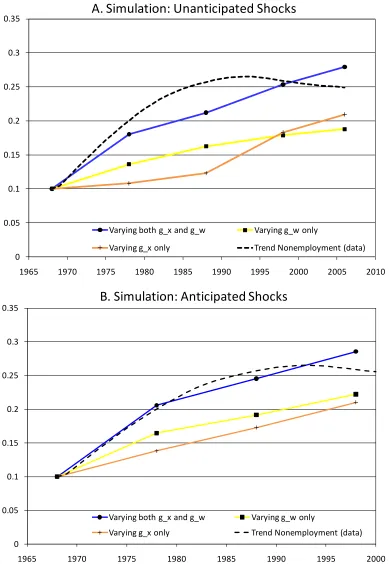
Figure 7A displays the results of this simulation based on these unanticipated shocks, together with the trend nonemployment rate among high school dropouts from Figure 1B for comparison. The model predicts a substantial rise in the nonemployment rate for low-skilled workers. Figure 7A reveals that the joint trends in gx( ) and gw together imply an increase in low-skilled nonemployment from 10 percent to 27 percent between 1968 and 2006. Comparing these outcomes to the observed trend from the data, this suggests that the model can account for all of the secular rise in nonemployment among high school dropouts over this period. Thus, variation in the returns to experience together with changes in the rate of aggregate wage growth have the potential to go a long way toward explaining the long-run variation in nonemployment for low skilled workers in the context of this model.
in the model. However, it also reveals that the e¤ects of gw are relatively more important earlier on, whereas the return to experience plays more of a role later on. This …nding is consistent with the trends depicted in Figures 2 and 3A. Declines in aggregate wage growth occur predominantly in the early part of the sample period, whereas declines in the return to experience among dropouts occur much more uniformly over the period.
Another feature of the results in Figure 7A is that the model is less successful in matching the observed timing of the increase in trend nonemployment among high school dropouts. The data reveal a substantial medium run rise in nonemployment in the 1970s and 1980s that the model does not fully predict. We do not necessarily view this as a problem, as it provides room for other explanations to play a role, a point we return to in Section V when we discuss how our explanation dovetails with prior literature.
The model’s inability to predict the medium run rise in joblessness also may be related to our choice to feed variation ingx( )andgw through the model as unanticipated shocks. It is possible that some of these changes may eventually have been anticipated. For example, workers may have become wise to the downward trend in aggregate wage growth seen in Figure 2. This would speed up the response of nonemployment to these shocks.
To highlight this point, we consider an alternative simulation. As before, the labor market is assumed to be in steady state at the beginning of the simulation in 1968. In this case, however, we assume that the time path of aggregate wage growth gw in Figure 2 is subsequently realized by all cohorts. Symmetrically, instead of using the cross sectional experience pro…les from Figure 3, we reveal smoothed versions of the realized experience pro…les to successive cohorts of workers.21
Figure 7B displays the results of this simulation based on theseanticipated shocks to wage growth. Consistent with the intuition above, it can be seen that implied nonemployment in the model tracks the medium run rise in nonemployment in the data remarkably well, though implied joblessness in the model overshoots the data in the late 1990s.
iii. Implications for Nonemployment by Skill
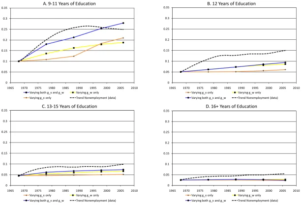
Up to now, we have focused on implied trends in joblessness among low-skilled high school dropouts. In this subsection, we compute implied trends in nonemployment rates for the remaining skill groups. Our simulation procedure mirrors exactly the method described above for high school dropouts. For each skill group, we feed the observed changes in the experience-earnings pro…le and aggregate wage growth in Figures 2 and 3 through the model as a series of unanticipated shocks. The only adjustment made is for di¤erences in the extensive elasticity of labor supply " across skill groups. The results of Section II.B. lead
us to expect that " declines with skill, as more skilled workers are less marginal to the employment decision. The estimates reported in Juhn, Murphy and Topel (1991, 2002) con…rm this intuition. Based on those estimates, we apply values of " equal to 0.2, 0.1, and 0.066 respectively for high school graduates, those with some college education, and those with a college degree or higher. Again, note that the e¤ects of di¤erent assumptions on the magnitude of these elasticities are simply to rescale our reported employment e¤ects up or down respectively.
Figure 8 plots trend nonemployment rates implied by our simulations, together with trend nonemployment rates from the data. Figure 8A repeats Figure 7A for ease of comparison. Figure 8 suggests that observed trends in experience-earnings pro…les and aggregate wage growth can account for around 5 of the 10 percentage point increase in nonemployment among high school graduates, and 3 of the 5 percentage point increase for those with some college education. Consistent with the relative stability of the experience-earnings pro…les for these groups in Figure 3, the majority of the implied increase in joblessness among both groups is driven by declines in aggregate wage growth. Figure 8 also reveals that trends in either form of wage growth can explain none of the 2 to 3 percentage point increase in nonemployment among college graduates. The reason, of course, the participation of high-skilled workers is not elastic because so few of them are on the work/non-work margin.22
iv. Implications for Overall Nonemployment
The simulation results allow us to gauge the extent to which variation in wage growth can account for the increase in aggregate nonemployment depicted in Figure 1A. We take a share-weighted average of the simulations in Figure 8. These simulated changes in the nonemployment rates by education group aggregate to 3.4 percentage points— a little more than half of the 6 percentage point rise observed in Figure 1A. Hence, taken together, the mechanisms identi…ed in the paper can account for all of the increase in nonemployment among white male high school dropouts, and for approximately one half of the increase in the aggregate nonemployment rate over between 1968 and 2006.
22In the working paper version of this paper (Elsby and Shapiro, 2009), we also explore the age structure
An important aspect of the simulations is that they take into account the dynamics of the adjustments to changes in growth in wages and the return to experience. As seen in Figure 6, these dynamics can be quite slow. Taking them into account is crucial for understanding the movement in employment rates. In the simulations, the upturn in wage growth has a very delayed e¤ect on aggregate employment rates owing to the decisions of older workers made well before the wage growth increased. Consequently, the upturn in wage growth exhibited in Figure 2 does not lead to a contemporaneous reversal of the decline in employment.
v. Implications for Nonparticipation
Until now, we have interpreted the predictions of the model as being aligned with secu-lar trends in nonemployment— the sum of nonparticipation and unemployment. This is motivated by in‡uential research noting that the distinction between unemployment and nonparticipation has become blurred at low frequencies, as low-skilled unemployed work-ers increasingly have become detached from the labor market, reporting very long spells of unemployment (Juhn, Murphy and Topel, 1991, 2002). However, as we noted in the introduction, an alternative view would be to interpret the labor supply margin that we model as corresponding to the participation margin. There are institutional, measurement, and theoretical considerations that potentially blur the distinction between nonparticipation and unemployment. While we incline to the the Juhn, Murphy and Topel perspective, the alternative perspective that the labor supply margin addressed by our model bears more directly on nonparticipation has substantial merit. Hence, in this subsection we explore the predictions of our model when viewed through the lens of trends in nonparticipation.
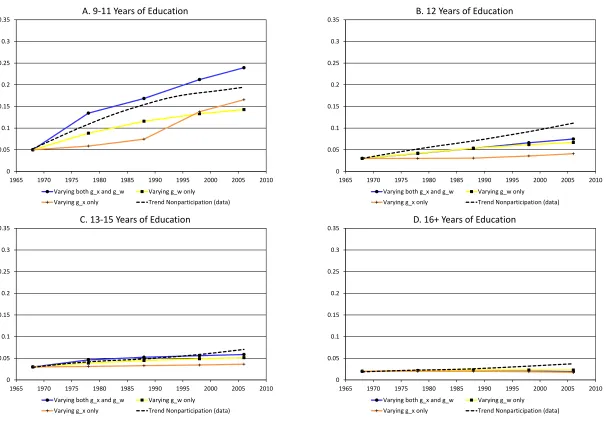
Our simulation approach mirrors the preceding analysis of nonemployment; the results are depicted in Figure 9. Nonparticipation among low-skilled high school dropouts is predicted by the model to rise substantially from 5 percent in the late 1960s to 24 percent in the mid 2000s. This tracks the increase seen in the data quite closely, though over predicts slightly the rise in nonparticipation by 2 to 4 percentage points over time. As in the results in Figure 8, declines in returns to experience and aggregate wage growth appear to account for roughly equal parts of the rise in low-skilled nonparticipation, with the productivity slowdown the more dominant earlier in the period.
school dropouts (Figure 3).
Taking a share-weighted average of these predicted e¤ects suggests that the model pre-dicts 4 of the 5 percentage point rise in aggregate nonparticipation among prime-age men. Thus, viewed from either the participation margin or the employment margin, the model is able to account for a substantial fraction of the rise in labor force detachment among American men since the late 1960s. The model is able to account for a larger fraction of the secular rise in nonparticipation than in nonemployment, however. The simple reason is that the long-run increase in nonparticipation across skill groups is slightly smaller than that for nonemployment.
V
Related Literature
This paper identi…es a novel explanation for why reductions in trend productivity growth are associated with secular declines in rates of employment. A natural question is how this new explanation contrasts with existing stories for the decline in male employment, and its coincidence with the productivity slowdown.
A
Search, creative destruction and capitalization e¤ects
As noted in the introduction, an important class of models of labor markets with frictions has explored the link between productivity growth and unemployment. As emphasized by Mortensen and Pissarides (1998), the predictions of these models rely crucially on the de-gree to which new technologies are embodied in newly-created jobs. In models of creative destruction (Aghion and Howitt, 1994), the productivity of a job is …xed according to the state-of-the-art technology available upon creation of the employment relationship. In order to update productivity back to the frontier, older relationships must be severed, hence “cre-ative destruction.” A drawback to models in this vein is that they can have counterfactual predictions with respect to the e¤ects of productivity growth on rates of worker realloca-tion and the level of unemployment (Blanchard, 1998). Viewed through the lens of these models, declines in productivity growth, such as the slowdown in the 1970s, imply that the rate at which jobs become obsolete slows, reducing job destruction, and thereby unemploy-ment. In contrast to these predictions, the productivity slowdown in the United States was characterized by increased rates of job destruction and increased unemployment.23
23For example, the data analyzed by Davis (2008) reveal that rates of job loss in the U.S. rose secularly in
If new technologies may be incorporated into jobs of all vintages, however, a capitalization e¤ect can arise (Mortensen and Pissarides, 1998). The idea is that the creation of new jobs involves the costly process of …lling a vacancy. These costs are borne upfront and are set against the stream of future pro…ts generated by the employment relationship. A slowdown in productivity growth raises the rate at which these future pro…ts are discounted, reducing the returns to job creation, and raising unemployment.24
The mechanism put forward in the present paper complements this capitalization e¤ect in a number of respects. First, the two approaches capture quite di¤erent aspects of the decline in employment that followed the productivity slowdown. The capitalization e¤ect noted by Mortensen and Pissarides (1998) emphasizes the impact of declines in trend growth on the demand for labor over the long run. In doing so, it seeks to provide an account of the rise in episodes of frictional unemployment that accompanied the productivity slowdown. In contrast, the view put forward in this paper provides an account of the decline in labor market attachment, and the concomitant rise in long jobless spells, that were observed in the wake of the slowdown in productivity growth. Accordingly, the emphasis in the present paper is on the e¤ects of aggregate wage growth on incentives to supply labor.
Second, the analysis of Section II.C. revealed that the existence of labor market frictions was likely to have only a modest e¤ect on the impact of wage growth on reservation wages that we emphasize. The absence of such interactions suggests that the implications of our theory are approximately additive with the capitalization e¤ects emphasized by Mortensen and Pissarides (1998), which operate through their e¤ects on labor market frictions, in particular the job-…nding rate.
Finally, the results of Section IV revealed that the model of this paper could account for the magnitude of the secular rise in nonemployment among the lowest-skilled education group. This is precisely the subgroup of the labor market on the margin of the work/non-work decision that experienced signi…cant rises in long jobless spells (Juhn, Murphy and Topel, 1991, 2002), which in turn is also the phenomenon our model seeks to encapsulate. In contrast, the model could account for around one half of the increase in aggregate nonem-ployment. The results of our quantitative analysis therefore leave room for other potential explanations, such as the capitalization e¤ect emphasized by Mortensen and Pissarides. In their quantitative analysis, Pissarides and Vallanti (2007) …nd that plausible calibrations of the capitalization e¤ect can account for part of the empirical relationship between
unem-24Manning (1990) identi…es a capitalization e¤ect in a di¤erent context within a dynamic model of union
ployment and trend growth, perhaps around one third.25 This, in turn, leaves room for the e¤ects emphasized in the present paper and vice versa.
Overall, this suggests that these two explanations are largely complementary, both in terms of being conceptually distinct, and in terms of their quantitative predictions.
B
Does the short run last a long time?
Perhaps because traditional models tend to predict no long run employment e¤ects of changes in productivity growth, a prominent feature of previous literature has been in its emphasis on the potential short run employment e¤ects of variation in productivity growth (see among others Blanchard, 2000; Bruno and Sachs, 1985; Ball and Mo¢ tt, 2001). A popular idea that has been pursued is that the wage demands of workers are somewhat sluggish in their response to changes in productivity growth. Blanchard (2000) has suggested that a “comprehension lag”can arise between the moment of an initial decline in productivity growth and the time that workers become aware of it. Similarly, Ball and Mo¢ tt (2001) have emphasized the possibility of sluggish “wage aspirations” that do not adjust immediately to declines in the sustainable rate of aggregate wage growth. Both of these possibilities will lead to a short run rise in joblessness. Moreover, depending on the sluggishness of reservation wages, the short run can last a long time.
A limitation to this approach, emphasized in Blanchard (1998), is that it becomes dif-…cult to explain very persistent declines in employment following a productivity slowdown, unless one is willing to impose extreme forms of sluggishness in reservation wages. Such a task becomes especially di¢ cult given the observed rebound in aggregate wage growth that accompanied the productivity “miracle”of the 1990s. Models of sluggish adjustment in reservation wages would predict reductions in joblessness in the 1990s. There was a decline in unemployment across the board in the late 1990s, though not for a long-enough period to change much the picture of trends in nonemployment shown in Figure 1. Interestingly, our model contrasts with these predictions. The results of Section IV imply that the pro-ductivity slowdown of the 1970s led to increased joblessness over long (thirty year) horizons, rather than short horizons. Thus, while models of sluggish adjustment in reservation wages may account for the short to medium run rise in joblessness in the 1970s and 1980s, our model can account for the persistent rise in nonemployment into the 1990s. Recall that this is driven by the important employment dynamics that are emphasized when one takes into account the e¤ects of human capital accumulation on work incentives over the lifecycle.
25Pissarides and Vallanti (2007) …nd that calibrations of the capitalization e¤ect can account fully for the
C
Skill-biased technical change and the decline in employment
A …nal related explanation of the secular decline in male employment rates does not appeal to the productivity slowdown, but rather to the concurrent rise in wage inequality in the 1970s and 1980s. Low-skilled workers in the United States experienced sustained declines in their real wages over this period (Bound and Johnson, 1992; Juhn, Murphy and Topel, 1991, 2002), a fact reiterated in Figure 2. This fact in turn suggests a simple explanation for the decline in low-skilled employment: If marginal workers face reductions in their wage, it seems intuitive that they would respond by withdrawing their labor supply (Juhn, 1992). Our analysis provides a number of interesting perspectives on this hypothesis. First, it is worth re-emphasizing that, since our model explains just part of the overall rise in trend nonemployment, other explanations play a complementary role. Consider the timing of the rise in nonwork predicted by our model compared to the timing of the rise in wage inequality. The decline in wages experienced by low-skilled workers starting in the 1970s halted by the early 1990s, and reversed signi…cantly later that decade (Juhn, Murphy and Topel, 2002). In contrast, our simulations in Section IV reveal that, while the model could account for the persistence of the rise in nonemployment into the late 1990s and 2000s, it under predicts the medium-term rise in the 1980s. Thus, there is room for a joint explanation of the overall decline in trend employment rates.
In addition to this, however, our model further highlights an important necessary con-dition for declines in the level of wages— such as those associated with the rise in wage inequality— to have an impact on employment rates: It must be that the payo¤ from non-work (denoted b in our model) did not fall in tandem with the wages of less-skilled workers. Prior literature often has assumed that it would, usually by appealing to the fact that un-employment compensation is often a …xed fraction of prior wages. To the extent that this were so, reductions in wage levels of low-skilled workers that accompanied the rise in wage inequality would have a muted e¤ect on employment. Assessing the extent to which replace-ment rates have risen over time, especially among the low-skilled, is therefore a worthy topic of future research.
VI
Conclusion
on work incentives. In