LINEAR PROGRAMMING MODEL FOR OPTIMAL CROPPING PATTERN FOR ECONOMIC BENEFITS OF MRBC COMMAND AREA

(1)

Linear Programming Model For Optimal

Cropping Pattern For Economic Benefits Of Mrbc

Command Area

Mahek Giri Aparnathi Prof. Divya k Bhatt

L.D Engineering college Ahmedabad L.D Engineering college Ahmedabad

Abstract

Optimal cropping pattern optimization model is formulated in which the surface and ground water as decision variables. Linear programming is used for multiple crop models and dynamic programming for single crop model. In irrigated agriculture, where various crops are competing for a limited quantity of land and water resources, linear programming is one of the best tools for optimal allocation of land and water resources (smith, 1973; mAji and heady, 1980; loucks et al., 1981. Salman et al (2001) present a linear programming model to derive regional water demands based on optimized regional cropping pattern with variable water prices based on quality.

Keywords: Horizontal Pressure Vessel, Design using PVElite, Local stress analysis using PVElite.

_________________________________________________________________________________________________________

I. INTRODUCTION

In this study, developed a crop allocation model that maximizes agricultural profits constrained by land by and water availability. The decision making unit on at the level of a single ditch, which maximizes net income by choosing the optimal cropping pattern, land and water usage, given input and output prices. Ey. The model finds the optimal cropping pattern and land usage for the Nadiad branch canal command of mahi command (Gujarat (India), given water availability.

Linear programming (LP) has been used extensively in the analysis of water resource systems and irrigation planning. Some examples are now presented. Mathematical models in irrigation planning and water pricing policies mathematical programming models can be used to determine optimal activity and resource input levels.

II. OBJECTIVEOFSTUDY:

 Integration of remote sensing based crop acreage in optimization model (linear programming model)



Using LP model to maximize net benefit from optimal cropping pattern with different extent of allocation of water from canal and tube wells.

III. MATHEMATICALMODELFORMULATION

Objective function: the objective function is to maximize net benefit from irrigated area which includes returns from the irrigated area and the operations costs for canals and tube wells.

A. Benefits from agriculture returns:

Evaluation of benefits from system is tough task for the system analyst, the benefits from agriculture can be computed after deducting expenses incurred in growing crops like seeds, pesticides, fertilizer and labour and surface and ground water cost for cultivation of crops.

The net benefits are obtained by:

Net profit = market value product - cost1 – cost 2.

Cost-1 = the expenditure on seeds, pesticides, fertilizers and labour. Cost-2= irrigation cost = net annual capital cost.

Here we are concerned about the cost 2 from the department of agriculture: the amount for cost 1 for each crop was obtained and deducted from the market value product.

So the above equation is simplified to: Net profit= benefit –cost 2.

j Benefits =  Aj YPAj VPPj

(2)

Where, Aj = irrigation area of jth crop. YPAj = yield per acre of jth crop. VPPj = value per Rs. of jth crop

B. Operation cost from canals tube wells

Annual capital cost of canal is calculates by

i Cost of surface water =  C Yi i = 1

Where, C = operation cost for canal system

Yi = flow diverted into canal during ith season. i

Cost of ground water =  C Ti i =1

In-which C = operation cost for tube well system. Ti = pumpage from tube well in ith season.

C. OBJECTIVE FUNCION SUBJECTED TO CONSTRAINTS:

Water diverted to canals in any season cannot exceed the canal capacity.

 Yi ≤ Y D 

In which,  = ration of peak to average demand=1.1 Y = canal capacity in cumecs=16.56 Cumecs

 = canal efficiency =0.70 D = canal running days, In Rabi=85 Ci ≤ 7740

Seasonal diverted to canal cannot exceed seasonal river flow at the canal head- works. Ci ≤ xi

In which, ci = flow diverted into canal in ha m during ith season. Xi = available water at head of canal in ha m in ith season. Ci ≤ 2855

Water pumped from tube wells in any season cannot exceed the tube well capacity.

 ti ≤ g D 

In which,  = ration of peak to average demand G= max capacity of well system.

 = tube well efficiency D = no .of days canal running. No.of open well=1380 No.of tube well=237

Average yield of tube well=1500 lpm=0.0250 cumec Average yield of open well =935 lpm=0.0157 cumec There fore quantum of water available for pumping. Open well 0.0157 × 1380=21.66 cumec

Tube well 0.025 × 237=5.925 cumec Total =27.59 cumec

Consider the efficiency of as 70% and assuming that tube well is operated for 65 days in rabi season. Therefore ,total discharge capacity of tubewell and open well in ha m.

= 27.59 ×0.7 × 65 × 8.64 1.1 =9860 ha m. T1≤ 9860

Water requirement for crops is met in each season. j

 Aj WR ij - Ө2 (Ө1Yi +Ti ) ≤ 0 j = 1

In which, WR ij =irrigation water requirement of jth crop in ith season Aj = irrigated area for jth crop.

Ө2 = 1 – SR2 – AR2 –ET2 Ө1 = 1 – SR1 – AR1 –ET1

ZONE SR(surface runoff) AR(Artificialrecharge) ET(evapotranspiration)

(3)

Irrigated zone 0.1 0.2 0.1

Table. 1: Percentage of abstractions in the canal zone,irrigated zone.

0.4A1+0.36A2+0.70A3-0.6(0.8 C1+T1) ≤ 0

SR1= fraction of water diverted to canals that is lost as surface runoff =5% AR1= fraction of water diverted to canal that is lost as aquifer recharge =10%

ET1= fraction of water diverted to canals that is lost as non-beneficial evapotranspiration=5% SR2= fraction of water diverted to canals that is lost as surface runoff =10%

AR2= fraction of water diverted to canal that is lost as aquifer recharge =20%

ET2=fraction of water diverted to canals that is lost as non-beneficial evapotranspiration=10% Case-a. Restricts maximum value for irrigation under each crop.

Aj ≤ TIA

In which Aj = irrigation area of jth crop TIA= total available area for irrigation.

A1 ≤ 9643 A2 ≤ 2594 A3 ≤ 2088

Case-b. Allow 25% variation in maximum value for irrigation under each crop without change in seasonal irrigation intensity. 0.75TIA ≤ Aj≤ 1.25TIA

In which Aj = irrigation area of jth crop TIA= total avai lable area for irrigation

7232 ≤ A1 ≤ 12053 1946 ≤ A2 ≤ 3566 1566 ≤ A3 ≤ 2610

Total area of various crops cannot exceed the total available area of irrigation. j

 Aj ≤ TIA j = 1

A1+A2+A3 ≤ 14325 In which Aj = irrigation area of jth crop TIA= total available area for irrigation

IV. EXECUTIONOFMATHEMATICALMODELWITHDIFFERENTINTENSITIESFORDIFFERENTRELEASE

POLICIES.

The aim of the present study is to determine optimal cropping pattern and optimal utility of ground water instead of existing cropping pattern considering socio-economic point of view.

Water release from canal may vary every year according to reservoir status as determined by rain in monsoon rain, so in place of actual water release policies of canal release. On the basis of past four years release.

Policy.1-2500 ha m,policy.2-2750 ha m,policy.3-3000 ha m,policy.4-3250 ha m of canal water for rabi season. Ground water resources can be utilized up to safe limit to satisfy with different proposed seasonal irrigation intensity of 30%,50%,70%,80%, and 100%.

Year/season Release in day cusec Release in M.C.F.T Release in M.C.M Release in ha m

2011-12/rabi seasons 11666 1079.94 28.54 2855.81

2012-13/rabi seasons 9878 853.46 24.16 2420

Table. 2: ACTUAL RELEASE FROM CANAL IN RABI SEASON

Year/season Release policy-1(ha m) Release policy-2(ha m) Release policy-3(ha m) Release policy-4(ha m)

2012-13/rabi season 2500 2750 3000 3250

Table. 3: PROPOSED RELEASE POLICY BASE OF ON PAST RELEASES RABI SEASON IN (ha m)

Table show that area to be irrigated foe each crop for 2 cases of constraints 5, respectively ,under different irrigation intensities.

Rabi crops Actual area irrigated (ha) Seasonal irrigation intensity 30% 50% 70% 80% 100%

Wheat 9643 4133 6888 9644 11021 13776

Tobacco 2594 1112 1853 2595 2965 3706

(4)

Table. 4: AREA TO BE IRRIGATED FOR EACH CROP (in ha) FOR DIFFERENT SEASONAL, IRRIGATION INTENSITY BASED EXISTING CROPPING PATTERN.

Rabi crops Actual area irrigated (ha)

Seasonal irrigation intensity

30% 50% 70% 80% 100%

Wheat 9643 4000-5166 5166-8610 7233-12055 8266-13777 10332-17220

Tobacco 2594 834-1390 1390-2317 1947-3244 2224-3707 2780-4633

Other 2088 672-1119 1119-1492 1567-2612 1791-2984 2238-3729

Table. 5:AREA TO BE IRRIGATED FOR EACH CROP (in ha) FOR DIFFERENT SEASONAL, IRRIGATION INTENSITY BASED EXISTING CROPPING

PATTERN UNDER THE CONSTRAINTS OF MAXIMUM VARIATION 25 %

V. THEMATHEMATICALMODELISDEVELOPEDINPREVIOUSTOPICISEXECUTEDFORFOLLOWING

CASES.

CASE-I. Existing and suggested cropping pattern for rabi season with different intensities for actual release of canal water.

CASE-II. Allow 25% variation in area under each crop for existing and suggested cropping pattern for rabi season with different intensities for actual release of canal water.

CASE-III. Suggested cropping pattern for rabi season with different intensities for different release of canal water.

CASE-IV. Allow 25% variation in area under each crop for existing and suggested cropping pattern for rabi season with different intensities for different release of canal water.

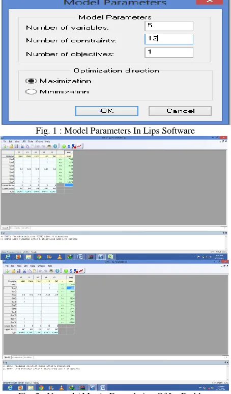
Fig. 1 : Model Parameters In Lips Software

(5)

VI. RESULT

The net benefit of the irrigation system under different scenarios as discussed earlier are presented in …., in case of actual release policy, table and table show net benefit for different seasonal irrigation intensity for case (a) and case (b) of constraint 5.

A. CASE-I

Existing and suggested cropping pattern for rabi season with different intensities for actual release of canal water.

Release policy Seasonal irrigation intensity Cost of S.W. Rs.(105_{) Cost of G.W Rs.(10}6_{) Net benefit(10}7₎

Actual Release

Policy

30% 3.8542 1.8443 7.9452

50% 3.8542 4.3605 13.1387

70% 3.8542 6.8778 18.3351

80% 3.8542 8.1349 20.9296

100% 3.8542 8.3317 22.0527

Table. 6: Net Benefit For Different Seasonal Irrigation Intensity For Actual Release (In Case-A .Aj<=Tia)

B. CASE-II

Allow 25% variation in existing and suggested cropping pattern for rabi season with different intensities for actual release of canal water.

Release policy Seasonal irrigation intensity Cost of S.W. Rs.(105_{) Cost of G.W Rs.(10}6_{) Net benefit(10}7₎

Actual Release

Policy

30% 3.8542 2.7880 9.8931

50% 3.8542 5.5659 15.720

70% 3.8542 8.3317 21.5677

80% 3.8542 8.3317 22.0538

100% 3.8542 8.3317 22.7180

Table. 7: Net Benefit For Different Seasonal Irrigation Intensity For Actual Release(In Case-B. 0.75tia ≤ Aj ≤ 1.25tia)

C. CASE-III

Suggested cropping pattern for rabi season with different intensities for different release of canal water.

D. CASE-IV

Allow 25% variation in area under each crop for existing and suggested cropping pattern for rabi season with different intensities for different release of canal water.

In case of different release policy, table shows net benefit for different seasonal irrigation intensity for case a and case b of constraints 5.

Release policy Seasonal irrigation intensity

Net benefit in Rs.(107₎ Case-iii

Aj ≤ TIA

Case-iv

0.75TIA ≤ Aj ≤ 1.25TIA

Release policy-1

30% 7.9260 9.8739

50% 13.0119 15.7013

70% 18.3159 21.1274

80% 20.8345 21.6134

100% 21.6124 21.8017

Release policy-2

30% 7.9395 9.8874

50% 13.1331 15.7148

70% 18.3295 21.4375

80% 20.9239 21.9235

100% 21.9225 22.4470

Release policy-3

30% 7.9531 9.9010

50% 13.1466 15.7283

(6)

80% 20.9374 22.2336

100% 22.0612 23.0923

Release policy-4

30% 7.9666 9.9145

50% 13.1601 15.7418

70% 18.3565 22.0577

80% 20.9509 22.5437

100% 22.0747 23.4424

Table. 8: Net Benefit For Different Release Under Different Seasonal Irrigation Intensity(Case-Iii, Aj ≤ Tia & Case-Iv 0.75tia ≤ Aj ≤ 1.25tia)

VII. DISCUSSIONOFRESULT

Fig 1 shows the net benefit for actual releasease policies under different irrigation intensity (30%,50%,70%,80% and 100% etc.) for both the case of constraint 5. As intensity of irrigation net benefit also increased. For same irrigation intensity the case II had higher benefit than the case I. in case I benefits ranged from 7.94 to 22.05 and case II benefits ranged from 9.89 to 22.77. release 4 had highest benefit in both the cases. As intensity of irrigation is utilization of ground water is also increase so cost of ground water is increase. Result of case-I and case-ii as shown in table.

Fig. 1: Net Benefits For Actual With Different Level Of Intensity

 IN CASE OF Aj ≤ TIA

 IN CASE OF 0.75TIA ≤ Aj ≤ 1.25TIA

Fig show 2 the net benefits for different release policies under 30% seasonal irrigation intensity the case IV had higher benefits than the case-III. In case-III benefits ranged from 7.92 to 7.96 and case IV benefits ranged from 9.87 to 9.91. release 4 had highest benefits in both the cases

Fig. 2: Net Benefits For 30% Seasonal Irrigation Intensity

Fig show 3 the net benefits for different release policies under 50% seasonal irrigation intensity the case IV had higher benefits than the case-III. In case-III benefits ranged from 13.01 to 13.16 and case IV benefits ranged from 15.70 to 15.74. release 4 had highest benefits in both the cases

0 5 10 15 20 25

Net Benefits for actual release

with different level of intensity

CASE-I

CASE-II

0 10

N

ET

B

EN

EFI

TS

(10

7)

NET BENEFITS FOR 30%

SEASONAL IRRIGATION

INTENSITY

(7)

Fig show 4 the net benefits for different release policies under 70% seasonal irrigation intensity the case IV had higher benefits than the case-III. In case-III benefits ranged from 18.31 to 13.35 and case IV benefits ranged from 21.12 to 22.05. release 4 had highest benefits in both the cases.

0 5 10 R EL EA SE … R EL EA SE … R EL EA SE … R EL EA SE … N ET B EN EFI TS (107)

NET BENEFITS FOR 50%

SEASONAL IRRIGATION

INTENSITY

CASE-III (Aj ≤ TIA)

CASE-IV(0.75TIA ≤ Aj ≤ 1.25TIA)

0 5 10 R ELE A … R ELE A … R ELE A … R ELE A … N ET B EN EFI TS (10 7)

NET BENEFITS FOR 70%

SEASONAL IRRIGATION

INTENSITY

CASE-IV(0.75TIA ≤ Aj ≤ 1.25TIA)

19 20 21 22 23 N ET B EN EFI TS (10 7)

NET BENEFITS FOR 80%

SEASONAL IRRIGATION

INTENSITY

(8)

VIII. SUMMARYANDCONCLUSION

The linear programming model was formulated for maximization of net return from optimal cropping pattern with conjunctive water use, considering various release policies and intensities of irrigation. It was found to be an effective tool for land and water resources allocation. The existing cropping pattern and its acreage in nadiad branch canal command area was estimated using multi-date remote sensing data of IRS P6/1D LISS-III. Based in this acreage the intensity of irrigation was suggested under each crop. The release policies canal was based on previous year’s taken from actual situation.

Following specific conclusions could be drawn using with regard to optimization of net return from optimal cropping pattern with conjunctive water use.

 The comparison of case –I and case-ii for actual release policy and existing cropping pattern. Showed that the net return in case-ii was higher as compared to case –I for same intensity of irrigation. This showed the existing cropping pattern was non –optimal.

 Comparison of results of case-iii and case-iv showed that the for different release policies under same intensity of irrigation the change in benefits is nominal. Hence the average of four release policies could be considered as the best scope of surface water and ground water utilization.

 For same intensity and same release policy, comparing case-iii and case-iv, the net return was higher in case-iv in which 25% variation was allowed in area under each crop.

REFERENCE

[1] Lakshminarayana,V.RAjagopalan P,..1977.Optimal Cropping Pattern For Basin In India. J Irri.Drainage Eng.Div.,Asce 103(1),Pp.53-70. [2] Khepar S.D And Chaturvedi M.C 1982’optimum Cropping And Ground Water Management’water Resources Bulletin Pp,655-660.

[3] De Wit, A.J.W.,&Boogaard, H.L (2001). Monitoring Of Crop Development And Crop Model Optimization Using Noaa-Avhrr: Towards In Integrated Satellite And Model-Based Crop Monitoring System In The European Context (Vol.Bcrs Report 2000:Usp-2 Report 2000:00-12). Delft:Beleids Commission Remote Sensing(Bcr).

[4] Paudyal,G.N and Gupta, A.D (1990).”irrigation planning by multilevel optimization” Journal of irrigation and drainage engineering. ASCE,116(2).273-291. [5] Raval,puskar (2004). Determination of optimal cropping pattern for conjunctive use of surface and ground water –A case study of matar branch canal, M.E

thesis wrm LDCE ahmedabad.

20 21 22 23 24

N

ET

B

EN

EFI

TS

(10

7)

NET BENEFITS FOR 100%

SEASONAL IRRIGATION

INTENSITY

CASE-III(Aj ≤ TIA)