Unifying the analysis of high-throughput sequencing datasets: characterizing RNA-seq, 16S rRNA gene sequencing and selective growth experiments by compositional data analysis

M E T H O D O L O G Y

Open Access

Unifying the analysis of high-throughput

sequencing datasets: characterizing RNA-seq,

16S rRNA gene sequencing and selective

growth experiments by compositional data

analysis

Andrew D Fernandes

, Jennifer NS Reid

, Jean M Macklaim

, Thomas A McMurrough

, David R Edgell

and Gregory B Gloor

Abstract

Background: Experimental designs that take advantage of high-throughput sequencing to generate datasets include RNA sequencing (RNA-seq), chromatin immunoprecipitation sequencing (ChIP-seq), sequencing of 16S rRNA gene fragments, metagenomic analysis and selective growth experiments. In each case the underlying data are similar and are composed of counts of sequencing reads mapped to a large number of features in each sample. Despite this underlying similarity, the data analysis methods used for these experimental designs are all different, and do not translate across experiments. Alternative methods have been developed in the physical and geological sciences that treat similar data as compositions. Compositional data analysis methods transform the data to relative abundances with the result that the analyses are more robust and reproducible.

Results: Data from anin vitroselective growth experiment, an RNA-seq experiment and the Human Microbiome Project 16S rRNA gene abundance dataset were examined by ALDEx2, a compositional data analysis tool that uses Bayesian methods to infer technical and statistical error. The ALDEx2 approach is shown to be suitable for all three types of data: it correctly identifies both the direction and differential abundance of features in the differential growth experiment, it identifies a substantially similar set of differentially expressed genes in the RNA-seq dataset as the leading tools and it identifies as differential the taxa that distinguish the tongue dorsum and buccal mucosa in the Human Microbiome Project dataset. The design of ALDEx2 reduces the number of false positive identifications that result from datasets composed of many features in few samples.

Conclusion: Statistical analysis of high-throughput sequencing datasets composed of per feature counts showed that the ALDEx2 R package is a simple and robust tool, which can be applied to RNA-seq, 16S rRNA gene sequencing and differential growth datasets, and by extension to other techniques that use a similar approach.

Keywords: compositional data, differential abundance, centered log-ratio transformation, Dirichlet distribution, Monte Carlo sampling, RNA-seq, microbiome, 16S rRNA gene sequencing, high-throughput sequencing

*Correspondence: [email protected]

2Department of Biochemistry, Medical Science Building, University of Western Ontario, 1151 Richmond St, N6A 5C1, London, ON, Canada

Full list of author information is available at the end of the article

Background

The objective of many high-throughput sequencing stud-ies is to identify those genes or features that make a significant difference between two or more conditions. These methods are diverse and include RNA sequencing (RNA-seq), chromatin immunoprecipitation sequencing (ChIP-seq), and metagenomic and 16S rRNA gene ampli-fication analysis of microbial populations. All of these study designs share common aspects whereby DNA frag-ments are incorporated into a library, a small proportion of that library is sequenced on an instrument and the reads from the sequencing run are binned into features that represent an underlying biological entity. The entities can be genes, other expressed or non-expressed genomic features (RNA-seq and metagenomics), operational tax-onomic units (OTUs) (16S rRNA gene sequencing) or genomic segments (ChIP-seq). Different statistical models are used to determine differential abundance in each type of study despite the underlying similarity in study design. The RNA-seq field has largely standardized on estimat-ing the variation with the negative binomial [1] and a relatively small number of normalization methods [2]. In contrast, the standard 16S tag-sequencing workflow nor-malizes abundances between samples by rarefaction or other subsampling methods and usually works with pro-portions [3,4], although some suggest that these normal-izations make little difference to the outcome [5]. Some groups additionally use quantitative PCR approaches to normalize reads [6]. Finally, ChIP-seq analyses often use Poisson-based models [7]. The methodological diversity appears to be due, in part, to historical accident as each field developed methods that derived from its own field of study and then became crystallized. The result is that methods used for one experimental design are often not suitable for another. However, all these tools treat the underlying data as counts per feature, adjusting these counts across samples and performing statistical tests on these adjusted counts [1,3,4,7]. Tools designed for one study design generally fail when applied to another (e.g., see [8,9]): this unexpected fragility suggests that the tools have been optimized to give biologically plausible results by latent parameterization.

Compositional data and high-throughput sequencing Despite current advice to treat high-throughput sequenc-ing datasets as count data [1,10], fundamentally, such datasets are compositional [8,9,11]. That is, the total num-ber of reads obtained for a particular sample is not itself informative. A dataset is compositional when the sum of the values for each sample is predefined [12]. Datasets of this type can be proportional, such as fractions of the whole, percentages, parts per million, etc. It is simplest to think of compositional values as being proportions of a unit, varying between 0 and 1. Proportional datasets

are very different from datasets composed of ordinary numbers that can take any value.

Treating high-throughput sequencing datasets as com-positions is intuitive if one considers that the primary determinant of the observed sequencing depth is the sequencing platform used and the number of samples that are multiplexed per run. For example, an Illumina HiSeq can currently generate over 200 million reads per lane, a MiSeq approximately 20 million reads per run and an Ion Torrent instrument up to 6 million reads per run. Setting aside confounding effects such as the accuracy of the instrument, clearly the direct comparison of different numbers of reads per category would be erroneous. Thus, we must think of datasets derived from high-throughput sequencing as compositions instead of count data. The purpose of this work is to show that datasets from a wide variety of experimental designs, including RNA-seq, 16S rRNA gene sequencing and selective growth (selex) experiments share a similar underlying structure, and can be analyzed appropriately using methods developed and used for decades in fields as diverse as geology, ecology and paleontology [12-15].

There have been many warnings regarding the use of standard statistical methods that assume the indepen-dence of the underlying observations when examining compositional data, the first being given by Karl Pearson in 1896 [16]. These warnings were ignored initially because there were no alternative methods. However, beginning in the late 1970s and continuing to this day, a number of approaches have been developed that fully use multivariate statistical approaches to examine compo-sitional differences between samples. In 1986, Aitchison [12] presented a full set of rationales and detailed descrip-tions of what follows.

for 16S rRNA gene analysis (mothur, qiime and VEGAN) and tools to analyze ChIP-seq.

Compositional datasets present several special chal-lenges. The first challenge is that compositional data must be analyzed in a scale-invariant way: that is, the answer should be the same whether the investigator is dealing with proportions, percentages, ppm or per feature val-ues where the total value is constrained to be the sum of the parts [12]. Compositional data are also dimen-sionless since they are proportions where the numerator and denominator have the same units. That data gen-erated by high-throughput sequencing approaches must be analyzed in a scale-invariant manner is implied by the various corrections for read depth used by the RNA-seq community [2], and by the rarefaction or jack-knifing commonly used by common 16S rRNA gene analysis tools [18]. The second challenge is that the count values for fea-tures in a sample are not independent. In these datasets the value of one feature necessarily restricts the value of at least one other, and in general restricts the val-ues of many others [9,12,16]. This property manifests as strong correlations between features, and was the origi-nal issue identified by Pearson [16]. The third challenge is that taking sub-compositions of such data often results in completely different interpretations of the correlation structure [12]. Aitchison gives simple examples of this effect where changing the abundance of one feature in a composition results in correlation between the others changing from strongly positive to strongly negative. This effect is problematic, given current guidance by popu-lar 16S tag-sequencing analysis tools to filter reads falling below a certain threshold [19,20] or for removing riboso-mal RNA sequences through chemical or computational means when performing RNA-seq.

Treating compositional datasets as ratios

Aitchison realized that the above constraints could be alleviated by investigating the ratios between proportions [12]. He developed a number of approaches that remove or reduce the above constraints, and with the proper inter-pretation, allow full use of standard statistical techniques. These transformations have been shown to increase reso-lution and allow more robust data interpretations in fields as diverse as paleontology [15], environmental sciences [14], metabolomics of wine [13], meta-transcriptomics [8] and 16S rRNA gene tag sequencing [9].

A conceptually simple transformation is the centered log-ratio transformation, or clr. Here the read counts for each feature are divided by the geometric mean of the read counts of each feature in the sample, followed by tak-ing the logarithm. The clr has the advantage that there is a one-to-one transformation of all features, allowing changes of all features to be observed. Moreover, if 2 is used as the base of the logarithm, then differences

between features represent fold-changes in relative abun-dance between features, a measure that is natural for molecular biologists, biochemists and other life scien-tists. Additional transformations have been developed by Egozcue and collaborators that have more robust prop-erties, but which lack a one-to-one mapping of the sam-ple features [21,22]. We will use the clr transformation throughout the remainder of the paper since this transfor-mation is the most widely used and simplest to interpret.

By way of example, consider the following set of values:

x = [10, 35, 50, 500]: where the proportional sum is con-strained to be 1. We could imagine that we have the counts from an RNA-seq experiment where the last feature is the count of reads mapping to ribosomal RNA. Converting to proportions,

px= 10, 35, 50, 500

595 =[0.0168, 0.0588, 0.0840, 0.8403], and the difference between elements 1 and 2 is−0.042: a very small difference. If we remove one observation (say the last one), equivalent to what is often done when removing the large number of sequences mapping to rRNA gene sequences from RNA-seq datasets, this changes the dataset to

px= 10, 35, 50

95 =[0.1052, 0.3684, 0.5263].

Now the difference between elements 1 and 2 is much larger, being−0.263, and the investigator could be led to a different conclusion. In contrast we can consider these same elements as compositions and compute the rela-tive difference between elements using the clr. In the case of the complete vector, the corresponding values (using base 2) are clr(x) = [−2.44,−0.64,−0.12, 3.20] and the difference between elements 1 and 2 is−1.81. If the com-position is reduced by removing the last element as before, then the corresponding clr values are [−1.38, 0.43, 0.94], and the difference is unchanged at−1.81. The meaning of this result is that element 1 is 2−1.81 as abundant as ele-ment 2. Thus, the same relative difference between these two elements is maintained regardless of which other element, or combination of elements, is removed.

the feature may be present, but below the detection limit imposed by the number of reads that are possible to achieve with the instrument. In the examples that follow, zero values are dealt with in two ways. First, by remov-ing a feature from consideration if the feature has zero counts in all samples. These features are inferred to be so rare that we can assume that sequencing more replicates would always result in zero reads being identified. Second, when one or more values of a composition is greater than zero, then all the values in the composition are retained even if they are zero. We then treat these remaining zeros in a Bayesian context [8,9] and assume that the reason no reads were detected in some features was because of sam-pling variance. The methodology by which this is done is outlined in the Methods Section, and the full method is implemented in the ALDEx2 R package [23].

Methods

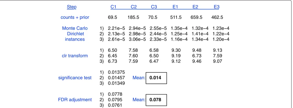
A pictorial summary of the method is outlined in Figure 1. Input data tables for ALDEx2 have i rows containing counts of values for each feature, andjcolumns represent-ing samples. Features that contain zero reads in all samples are removed as they are considered uninformative, and by definition are unable to contribute to the pool of differ-entially abundant features. Similar strategies are standard in RNA-seq analysis where rows summing to less than some value are excluded as they cannot be tested reliably for overdispersion [24]. Similarly, the standard practice in 16S rRNA gene sequencing is to exclude features that are

less than an abundance cut-off [19,20], and in practice this usually means excluding singleton reads. The problem is most acute when examining RNA-seq data since struc-tural, ribosomal, transfer and other RNA sequences are physically or computationally depleted prior to analysis. It is crucial to note that when the values in a com-positional dataset are manipulated in this way the data transformations proposed by Aitchison and used here are required to prevent spurious conclusions because of sub-compositional incoherence in sub-compositional data [12]. The total number of reads for all features in a sample

Nj = ini,jis not a predictable outcome of the experi-mental design because it is dependent on the instrument capacity and the number of samples that are multiplexed in the run. The actual number of counts for a given fea-ture are therefore not of interest and are generally scaled [2]. Note that along with the total counts per sample, the total number of counts does provide information about the precision of per feature count estimation [8,9].

Normalization across samples can be achieved using maximum likelihood to give a single estimate of the pro-portion of reads per feature,pi,j = ni,j/ini,j. However, this simple normalization has several flaws, mainly that both high and low count features may not be estimated correctly [2,25]. The number of reads per feature can be modeled as being sampled from a multinomial Poisson process, and the approach that performs best is to model the read counts as being derived from a Dirichlet process [8,9,26,27].

counts + prior

Monte Carlo Dirichlet instances

clr transform

FDR adjustment Step

69.5 185.5 70.5 511.5 659.5 462.5

2.21e 5 2.94e 5 2.55e 5 1.35e 4 1.32e 4 1.23e 4 2.13e 5 2.98e 5 2.44e 5 1.25e 4 1.41e 4 1.22e 4 2.61e 5 3.06e 5 2.33e 5 1.16e 4 1.34e 4 1.20e 4

6.50 7.58 6.58 9.30 9.48 9.13 6.45 7.60 6.50 9.19 6.73 7.59 6.73 7.59 6.47 9.12 9.46 9.07

0.01375

0.01457 Mean: 0.014

0.01349

0.0778

0.0795 Mean: 0.078

0.0761 1) 2) 3)

1) 2) 3)

1) 2) 3)

1) 2) 3)

C1 C2 C3 E1 E2 E3

Figure 1 shows a worked example for a single featurei for three control (C) and three experimental (E) samples. First, sequences that map to each feature are enumer-ated and the table of read counts for each feature in each sample is converted to a distribution of posterior proba-bilities through Monte Carlo sampling from the Dirichlet distribution for each sample:

p[n1,n2,. . .]|N =Dir

[n1,n2,. . .]+1 2

.

An uninformative prior of 1/2 is used to model the fre-quency of features with zero counts [28,29]. This prior maximizes the information in the data while minimizing the effect of the prior on the posterior in the case where the relative frequencies of each feature are of equal impor-tance [29]. Usually, 128 Dirichlet Monte Carlo (DMC) instances are sufficient since we are concerned only with summarizing central tendencies, not tail-related events. Each point value is now represented by a vector of poste-rior probabilities,pi,j[1, 2,. . .]. The distributions are nar-row if the feature and the sample contain a large number of counts and wide if either the feature or the sample has a small number of counts. Each Monte Carlo realization of

pi,jis transformed by the clr transformation:

ci,j=log2(pi,j)−mean log2(pj).

After this transformation the value for each feature is now relative to the geometric mean abundance of all val-ues in the sample. We will refer to clr-transformed valval-ues as relative abundance values, and to untransformed val-ues as proportional valval-ues throughout. Each realization of theci,jvalue between conditions is subjected to both a Welch’st-test and a Wilcoxon rank test giving two vectors ofP values, and eachP value instance is then corrected for multiple hypothesis testing using the false discovery rate (fdr) approach of Benjamini and Hochberg [30]. The expected value of thePand fdr statistics are then reported for both statistical tests.

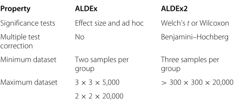
ALDEx2 also returns the within- and between-condition measures and the effect size that was used by the original version of ALDEx [8]. However, these statis-tics are calculated in a much more efficient way allowing near arbitrarily sized experimental designs. The major dif-ferences between ALDEx2 and the original version are outlined in Table 1.

The default parameters of ALDEx 2.0.6, DESeq v1.14.0 [31], DESeq2 v1.2.8 [31], SAMseq v2.0 [32] and baySeq v1.16.0 [33] versions were used in R version v3.0.2 [34].

Results and discussion

We will use example datasets that are sufficiently different to show that the concepts are generalizable to many types of high-throughput sequencing studies including selective

Table 1 Comparison of ALDEx and ALDEx2

Property ALDEx ALDEx2

Significance tests Effect size and ad hoc Welch’stor Wilcoxon

Multiple test No Benjamini–Hochberg

correction

Minimum dataset Two samples per Three samples per

group group

Maximum dataset 3×3×5,000 >300×300×20,000

2×2×20,000

Dataset: samples in A×samples in B×number of features.

growth experiments, RNA-seq, ChIP seq, 16S rRNA gene tag sequencing and others.

Examining selective growth experiments

Selective growth experiments (selexes) are often used to identify sequence variants for genes that confer a growth phenotype upon the cell line containing them. In this type of experiment the investigator is interested in identifying the fold enrichment of variants that exhibit some activity.

The first dataset is a single-round enrichment exper-iment testing the activity of a library of LAGLIDADG homing endonuclease sequence variants [35]. This dataset is available within the ALDEx2 package. In this experi-ment two codons in the gene were randomized completely and two codons were free to encode only two acid amino acids. The total library was thus 1,600 possible quadruple amino acid variants. An active enzyme results in cleav-age of the gene for a bacteriostatic DNA gyrase toxin. DNA sequencing was used to collect data on the growth characteristics of cells containing individual variants in the library under both selective and non-selective (i.e., no toxin) conditions. Seven replicate experiments for activ-ity were conducted. With this experimental design it is expected that the relative abundances of each variant after growth in the non-selective condition would reflect the input abundances and vary only by sampling differences. Crucially, because the toxin is bacteriostatic, the relative abundances of each variant under the selective conditions should also reflect the input abundances since all vari-ants should survive but no variant should be able to grow. Thus, their relative abundance would be unchanged. In contrast, variants that allow escape from the selection would become relatively more abundant, but no variant becomes less abundant.

Carlo replicates of the Dirichlet distribution and the effect of sample size on power.

Analyzing selective growth data as counts

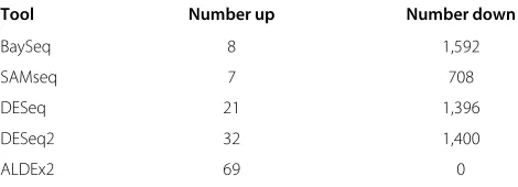
Among the most developed tools to examine high-throughput sequencing experiments are those designed to examine RNA-seq experiments [1], and these tools are often advocated for use in other experimental designs that generate tables of counts. These tools assume the data are counts of features for each sample and scale the counts to account for sequencing depth. The variance of each feature is calculated from a negative binomial model. We started with the hypothesis that existing tools used to examine RNA-seq experiments would be appropriate to identify those variants that exhibit differential growth. We tested this hypothesis using DESeq, DESeq2 [1], SAMseq [32] and baySeq [33] to identify differentially abundant variants. Table 2 shows that an examination of the data at a fdr of 5% indicated that the majority, or in some cases all, of the amino acid variants exhibited a significantly different frequency pre- and post-selection with each of these tools. All four tools identified a small number of fea-tures as becoming more abundant, and a large number of features as becoming less abundant. This makes sense in the context of counts, but not in the context of relative abundance because the vast majority of variants do not change their relative abundance under the selective condi-tions. Therefore, the differential growth exhibited by the variants under the selective and non-selective growth con-ditions clearly does not fit the underlying assumptions of any of these tools.

Analyzing selective growth data as compositions

The analysis that follows uses the clr transformation, described in the Methods, which converts the data from absolute differences to relative differences. Data trans-formed by the clr are centered on the geometric mean, with negative values being less abundant than the mean in that sample and positive values being more abundant than the mean. The difference between two values is the fold-change between them if the transformation is done using base 2 logarithms. One important property of the clr transformation is that the transformed values are inherently normalized for the sequencing effort [8].

Table 2In vitroselection experiment analysis of commonly used differential expression tools

Tool Number up Number down

BaySeq 8 1,592

SAMseq 7 708

DESeq 21 1,396

DESeq2 32 1,400

ALDEx2 69 0

Several groups have recently shown that the sampling error inherent in high-throughput sequencing protocols can be modeled appropriately by Monte Carlo sampling from a Dirichlet distribution [8,9,26,27]. Each instance sampled from a Dirichlet distribution is equivalent to assuming that read proportions for each feature are derived from a Poisson distribution with the additional constraint that the sum of the proportions of all compo-sitions must sum to 1 after sampling [28]. This approach gives a more accurate assessment of the expected value of the proportion for a given composition, and a correspond-ingly more accurate estimate of the expected value of the associated statistical values [8,9]. Monte Carlo instances can be drawn from the Dirichlet distribution and each Dirichlet instance is an estimate of the per feature propor-tion that would be observed if the same library had been sequenced again [8]. In effect, each Dirichlet instance is an equally valid outcome of the sequencing run based upon the total number of reads observed and their per feature distribution. One consistent problem with conducting experiments where there are hundreds or thousands of features is that the number of hypothesis tests conducted are greater than the degrees of freedom allowed by the number of replicates. This problem, in addition to the large uncertainty in accurately measuring the frequency of low-abundance features, means that it is very easy to underestimate the true underlying variation in the data, and to overestimate statistical significance [8,9].

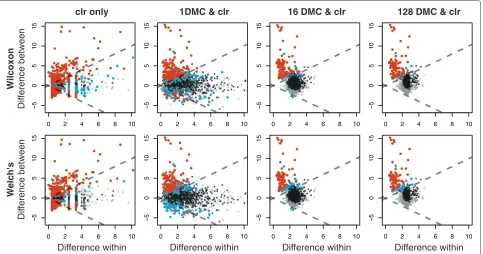
Figure 2 shows plots of the between-condition variation versus the within-condition variation (MW plots) [8] for clr-transformed data alone, or with the expected valued derived from differing numbers of DMC instances. Note that the MW plots show that there are many more ‘signif-icant’ features (red) when the clr transformation is used in the absence of DMC instances (clr only) or when there is only a single DMC instance than when the expected val-ues of the test statistics are determined from 16 or 128 instances. This occurs with both statistical tests.

Dif

ference between

Difference within

Dif

ference between

Difference within Difference within Difference within

W

ilcoxon

W

elch's

clr only 1DMC & clr 16 DMC & clr 128 DMC & clr

0 2 4 6 8 10

50

5

1

0

1

5

0 2 4 6 8 10

50

5

1

0

1

5

0 2 4 6 8 10

5

05

10

15

0 2 4 6 8 10

50

5

10

15

0 2 4 6 8 10

50

5

10

15

0 2 4 6 8 10

5

0

5

10

15

0 2 4 6 8 10

50

5

1

0

1

5

0 2 4 6 8 10

50

51

0

15

Figure 2Effect of DMC sampling on the selex dataset.The first column shows the results when the data is clr transformed without DMC sampling, the next three show the effect of 1, 16 and 128 DMC samples followed by the clr transformation. Features that pass a thresholdP<0.05 are shown in cyan and those where the fdr statistic is<0.05, are shown in red. Features where the median clr value is below the geometric mean are highlighted in black if they are not significant. Those where the median clr value is greater than the geometric mean are shown in gray. clr, centered log-ratio; DMC, Dirichlet Monte Carlo.

the right, being on average almost twice as variable in this procedure than when only the clr transformation is performed.

Table 3 enumerates the number of low-abundance features identified as significant as a fraction of the total number of significant features and the number of Monte Carlo samples from the Dirichlet distribu-tion (DMC). Note that low-abundance features com-pose a large fraction of all significant features when the clr only is used and when only a single DMC is used. Both the total number of significant features and the contribution of low-abundance features drops rapidly when DMC replicates are used to estimate the sam-pling variation. This is similar to the observation of Friedman and Alm [9], who demonstrated that examin-ing expected values of test statistics derived from DMC

Table 3 Effect of Dirichlet Monte Carlo instances on significance of low-abundance features

DMC Wilcoxona _Welch’sa

0 339/478 349/546

1 41/164 27/111

16 1/84 0/68

128 0/85 0/69

DMC, Dirichlet Monte Carlo replicate number.

a_{Number of low-abundance significant features/total.}

sampling significantly reduced the number of false posi-tive correlated features in 16S rRNA gene tag sequencing experiments.

One shortcoming of the clr transformation is that it may not transform the data such that it is normally distributed. In this case it may be more appropriate to use a non-parametric significance test to determine the difference between conditions. The top and bottom rows in Figure 2 show the results of Wilcoxon tests or of Welch’s t-tests on the clr-transformed values. We found that there was very good agreement between features identified by both statistical tests when using all seven replicates since all 69 features identified by the Welch’st-test were in the 85 features identified by the Wilcoxon test in the 128 DMC analysis using all seven replicates at a fdr<0.05. However, when only three of the seven replicates were included, no features were identified as significant by the Wilcoxon test while 16 features were still identified as signifi-cant by Welch’st-test. We therefore recommend Welch’s

t-test as its power is not as sensitive to sample size as the Wilcoxon test, although both test statistics are reported by ALDEx2, and the user should examine the results of both tests.

Examining the results of count vs composition analysis

identified as becoming relatively more abundant, and, in contrast to the other tools, no features are identified as becoming relatively less abundant. That DESeq, DESeq2, SAMseq and baySeq identify features that become less abundant makes sense if the data are counts, but do not make sense if the data are compositional. Recall that the design of the experiment was to identify those sequence variants that exhibited differential effects in a bacteriostatic growth assay. Thus if a variant was non-functional the abundance of the variant would be unchanged in the selected condition; i.e., cells contain-ing a non-functioncontain-ing variant would not grow and so these cells would remain at the input concentration until sampled. Conversely, if a variant was functional, cells containing it would grow and become much more abun-dant than average under the selective conditions. Note that cells containing both functional and non-functional variants would grow at the same rate and so the expec-tation is that variants would be found at approximately the same abundance under non-selective conditions. By way of illustration consider two variants from the dataset. The first variant K:D:I:E is non-functional, the counts for non-selected cells are [149, 89, 165, 68, 135, 128, 199] and for selected cells are [0, 0, 1, 0, 1, 0, 0]. Here the counts are very different, leading to the conclusion that this feature is less abundant in the selected than the unse-lected dataset, and this is reported as such by all tools (fdr for DESeq and baySeq are 3.8 × 10−7 and 1.8 × 10−4, respectively). However, relative to all other

vari-ants the counts for this variant are almost equal to the geometric mean abundance in both the selected and non-selected conditions: ALDEx2 reports an fdr of approximately 0.8 indicating no difference relative to the mean abundance under each condition. The second vari-ant, S:E:G:D, is weakly functional and the counts for non-selected cells are [755, 554, 669, 797, 862, 650, 2170] and for selected cells are [4710, 995, 906, 1716, 784, 804, 641]. This variant is identified as non-signficant by DESeq (fdr = 0.73), but is considered significant by ALDEx2 (fdr< 1×10−3). The difference is presumably because the counts are similar in the selected and non-selected conditions (DESeq log₂(fold-change) =22.9), but the rel-ative abundances are very different (ALDEx2 diff.btw.q 50=26.2).

We conclude that these tools, and by extension the many similar tools that use count-based methods to estimate variation [2,36], are inappropriate as general-purpose tools to examine differential growth experi-ments of this type. In contrast the clr transformation in combination with Dirichlet sampling indicated that only a minority of the variant combinations were under strong positive selection, a result that was in agreement with the biochemical characterization of the variants [35].

Analyzing RNA-seq data as compositions

The second dataset was generated by Bottomlyet al. [37] and contains 10 biological replicates of RNA isolated from the brain striatum from one mouse strain (C57BL6J) and 11 biological replicates of another strain (DBA/2J). The dataset contains an average of 22 million reads mapped for each sample. It was accessed from the ReCount dataset [38] in January 2014. The final output from ALDEx2 is available as Additional file 1.

RNA-seq attempts to address the question: ‘What are the differences between gene expression in the samples in two or more conditions?’ It is reasonable to exam-ine gene expression values as fold-change (relative dif-ferences) because the law of mass action that governs biochemical reactions depends on the ratios of reactants. For this reason, existing RNA-seq analysis tools report changes in gene expression as fold differences, despite computingPvalues as differences in scaled counts. What is not often appreciated is that gene expression is itself a limited resource in the cell, meaning that the tran-script abundance should also be modeled as proportional [39]. Furthermore, it is standard practice in the field to sequence only a subset of the total RNA in a sample: typically only the mRNA or some types of non-coding RNA are sequenced and rRNA and tRNA are excluded. This approach dramatically alters the sub-compositional structure of the data, potentially leading to non-robust inferences as discussed in the introduction.

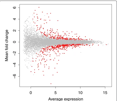
Differential expression in RNA-seq datasets is often visualized globally by Bland-Altman plots [40], which show the mean difference (M) vs average expression (A) (MA plots). An example MA plot derived from the DESeq package [31] for the large RNA-seq dataset presented by Bottomlyet al. [37] is shown in Figure 3. In this figure the points corresponding to the genes identified as differ-entially expressed are colored red. Note the relationship between fold-change and mean expression: genes with a small fold-change require high expression, and genes with a low expression value require a high fold-change to be identified as differentially expressed. Note also that for a given fold-change and expression value, the majority of genes with a greater fold-change and expression value are identified as differentially expressed. This MA plot is typ-ical of well-behaved datasets and such an idealized MA plot suggests that the analysis by this tool is valid. In this dataset 604 genes were identified as differentially abun-dant between conditions by DESeq using an fdr cut-off of 0.05.

The MA plot in Figure 3 was plotted using values out-put by DESeq, which assumes that the underlying data was count data and not compositional data [1]. We examined the similarity between the DESeq and ALDEx2 underly-ing values in two ways. First, by comparunderly-ing the DESeq corrected mean count values and the ALDEx2 median abundance values, and by comparing the DESeq and ALDEx2 fold-change values. There was an almost per-fect linear relationship for both these examples, with a Spearman correlation of >0.99 in both cases. Second, we replotted the values from DESeq onto clr space, and

0 5 10 15

−6

−4

−2

0

2

4

6

Average expression

Mean f

old change

Figure 3MA plot for DESeq.The base 2 logarithm of average expression across all samples for a feature is plotted vs the base 2 logarithm of fold-change. Points that are significantly different with a fdr less than 0.05 are in red, all others are in gray.

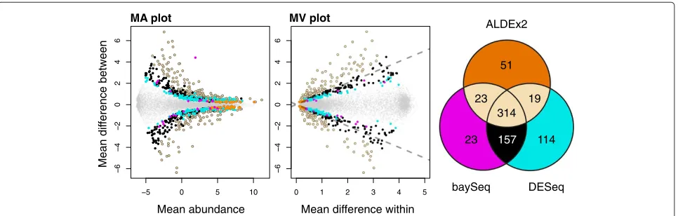
show these plots in the two left panels of Figure 4. In this figure features identified as significant by DESeq, baySeq and ALDEx2 individually and in common are highlighted in different colors: features identified as significant by DESeq are given by the filled light yellow circles along with the filled black and cyan circles; features identified as significant by baySeq are given by the filled light yellow circles and the filled black and magenta circles; and fea-tures identified by ALDEx2 (and at least one of the other two tools) are given by the filled light yellow circles and the orange filled circles. It is obvious from the left panel that the majority of genes identified by DESeq and baySeq as differentially expressed are consistent with the remapped sample space.

The MW plot panel in Figure 4 shows how the vari-ation in the dataset is distributed within and between conditions. In this plot the position where there is equal variation within and between conditions is shown by the dashed lines. The coloring is the same as for the left panel. The MW plot shows that a large fraction of the significant genes identified by both DESeq and baySeq (in black), by DESeq only (in cyan) or baySeq only (in magenta) exhibit as much or more within-condition vari-ation than between-condition differences. This is not a statistically desirable result. The genes identified as dif-ferential by DESeq or baySeq individually tend to be even more variable within a condition than those identified by both tools. In contrast, the significant features identified by ALDEx2 (in black and orange) always have a larger between-condition difference than within-condition dif-ference. Those genes that are uniquely identified by ALDEx2 (in orange) are almost exclusively genes with very high expression and relatively small differences between conditions.

The number of significant features identified by DESeq, baySeq and ALDEx2 is presented in a Venn diagram in the third panel of Figure 4. It is apparent that all three meth-ods identified approximately the same number of genes as being differentially abundant (ALDEx2 407, baySeq 517, DESeq 604) when controlling for an fdr of 0.05, and between 52% and 77% of the genes identified by one method were identified by all three. In summary, it can be seen that the expected value of thet-test for DMC-sampled and clr-transformed data ensures that the genes identified as differentially expressed exhibit a greater gene expression difference between mouse strains than the gene expression variation within either mouse strain. This example shows that the compositional analysis approach works well for RNA-seq datasets.

Analyzing 16S rRNA gene tag sequencing data as compositions

ALDEx2

baySeq DESeq

23 114

23 19

314

157

MA plot MV plot

Mean abundance

Mean dif

ference between

Mean difference within

51

5 0 5 10

6

4

20

2

4

6

0 1 2 3 4 5

6

4

20

2

4

6

Figure 4Differential features in common between ALDEx2, DESeq and baySeq.Genes are colored in light yellow if ALDEx and at least one of the other two tools identified them as significantly different with an fdr<0.05, black if they were identified by both baySeq and DESeq, magenta if only by baySeq, cyan if only by DESeq, and orange if only by ALDEx2. Small gray dots are non-differential genes. The Venn diagram illustrates the number of differentially abundant genes identified by each method. MA, mean difference between conditions vs average expression; MW, mean difference between conditions vs maximum within-condition variance.

10 January 2014 [41]. This dataset is a highly curated and annotated set of 16S sequence counts collected from a large number of people and a large number of body sites. We chose to examine the microbiota composition dif-ferences between the tongue dorsum and buccal mucosa because these sites had been shown to have somewhat dif-ferent microbial compositions both by a comprehensive analysis of the same 16S rRNA gene data and by an inde-pendent shotgun metagenomics analysis [42]. Since both approaches identified substantially similar taxa as differ-entially abundant, we were interested to determine if the relatively simple procedure implemented here could reca-pitulate the analyses done previously. The final output from ALDEx2 is available as Additional file 2.

The Human Microbiome Project dataset contained 23,393 OTUs containing one count or more for any of the 316 samples from the tongue dorsum and 312 sam-ples from the buccal mucosa. This dataset was analyzed with 16 DMC instances rather than 128 because of time and memory constraints, and because the analysis above suggested that 16 DMC samples would provide suffi-cient selectivity on low-count OTUs. The analysis was completed over all 23,393 OTUs in the dataset in approx-imately 76 minutes on a computer with 16 Gb RAM and an i7 processor. We observed 755 differentially abundant OTUs that had a Benjamini–Hochberg fdr< 0.05, and collected the 53 OTUs that passed that fdr cut-off with absolute effect size> 0.6. These 53 OTUs are displayed on the heat map in Figure 5.

The results show that OTUs assigned to the genera

Actinomyces,PrevotellaandVeillonellahave an increased relative abundance in samples from the tongue dorsum, while OTUs assigned toHaemophilusandGemellahave an increased relative abundance in samples from the

buccal mucosa. Several distinct OTUs assigned to

Strep-tococcus had different relative abundances in both body sites, although, in general OTUs assigned to this genus were over-represented in the buccal mucosa. Together, these results are congruent with those of Segata et al., who observed that these genera differentiate these body sites [42]. We conclude that the statistical procedure is also applicable to identify taxa that are differentially abundant between two samples in 16S rRNA gene tag sequencing experiments.

Conclusions

High-throughput sequencing is increasingly used to iden-tify differences between datasets composed of DNA or RNA sequences. Here we show that data transforma-tions appropriate for compositional data [12] can be used with standard statistical inference tools, such as Welch’s

t-test or the non-parametric Wilcoxon test, to identify features that are differentially abundant between condi-tions in datasets derived from selexes, RNA-seq or 16S rRNA gene segment sequencing. Historically, each of these experimental designs has used a distinct statistical model to determine significance when examining differ-ence between conditions, despite these experiments gen-erating similar types of data comprising large numbers of reads that are binned into one or more categories.

0 10 Value

Color Key

Actinomyces Gemella Granulicatella Haemophilus Lactobacillales Prevotella Streptococcus Veilonella

T

ongue

Buccal mucosa

OTUs

Figure 5OTUs with different relative abundances between tongue dorsum and buccal mucosa.Each OTU is colored by membership in the taxonomic level indicated. OTU abundance values are median relative abundance values derived from ALDEx2. OTU, operational taxonomic unit.

However, in their approach sampling is performed using a Poisson model that does not enforce a constant sum constraint, and they use the Wilcoxon rank test, which requires a large number of samples for statistical power. Furthermore, SAMseq treats the data as counts rather than compositions. Nevertheless, this method was shown to be superior to existing RNA-seq analysis tools based on Poisson or negative binomial models [32]. While this approach is superior in some ways to existing RNA-seq analysis tools on specific datasets, this tool set does not translate well to other experimental designs as shown in Table 2. In addition, RNA-seq analysis tools differ in how the values in the data are scaled between samples, and there is debate in the literature as to which scaling method is generally superior [2]. Finally, modeling has failed to reveal the ‘best’ tool because the tool that performs the best varies widely when the parameters of the model are altered [36].

For 16S rRNA gene sequencing, although the tools used to determine differential abundance between conditions are still evolving rapidly, no tool treats the data as com-positions and ensures sub-compositional coherence. For example, one widely used method [5] is similar to SAMseq in that it models the reads as coming from an under-lying Poisson model to estimate technical variance and identifies as differential those features that show signif-icance that is not sensitive to the estimated variance.

However, this method treats the values as proportions and not as compositions. Another commonly used trans-formation in 16S rRNA gene sequencing is the Hellinger transformation [43] implemented in the VEGAN R pack-age [44]. This transformation is also count based and is not sub-compositionally coherent.

Demonstration of the superiority of analysis methods is limited by two main factors: the first is that the abun-dance of a feature in a sample is a continuous variable, and the second is that there is often no objective standard to determine what is differentially abundant. Without

a priori information on what constitutes a biologically meaningful difference, there is no clearly demarcated line-in-the-sand that can be drawn between differential and non-differential abundance in any experimental design. Moreover, the relatively high cost of sequencing has led to study designs that often emphasize per sample sequenc-ing depth over biological replication [45], despite advice to the contrary [46,47]. This has led to the development of tools that attempt to estimate the biological variation from limited numbers of replicates.

The approach used in this paper models the reads per feature as proportions, acknowledging that the total sum of reads for a sample is not itself important. The precision of estimation of the proportional values is determined by taking Monte Carlo instances sampled from the Dirichlet distribution, which takes into account the number of reads per feature and the total sequencing depth. This approach generates narrow distributions when the read count is high per feature and per sample. The proportional data are transformed using the clr transformation, allowing standard statistical tools to be applied to each instance. Summary statistics are then reported as the expected value of the distributions.

We show that this approach is generalizable to three completely different experimental designs: a selex, an RNA-seq type experiment and a 16S rRNA gene amplicon-sequencing experiment. For the selex exper-iment, the ALDEx2 approach identified known active enzyme variants and weeded out inactive variants [35]. ALDEx2 identified a set of operational taxonomic units differential between two closely positioned body sites con-sistent with the results of two independent methods in the literature [42]. For RNA-seq, the ALDEx2 approach identified essentially all genes found by both DESeq and baySeq where the inter-condition difference was larger than the intra-condition variance. We believe that ALDEx2 exhibited greater specificity and equivalent sen-sitivity as these widely used tools.

Additional files

Additional file 1: Excel file containing ALDEx2 output for the Bottomly RNA-seq dataset.Column 1 contains gene features from the mouse genome. Column 2 contains the relative abundance of each feature averaged across all samples. Columns 2 and 3 contain the average relative abundance of DBA/2J and C57BL6J gene expression. Columns 4 and 5 contain the median between- and within-condition differences. Column 6 contains the median effect size. Columns 7 and 8 contain the expected values ofPand the associated Benjamini–Hochberg corrected fdr values for Welch’st-tests and the final two columns contain the expected values for Wilcoxon tests.

Additional file 2: Excel file containing ALDEx2 output for the buccal vs tongue dorsum comparison.Column 1 contains HMP OTU identifier labels. Column 2 contains the relative abundance of each feature averaged across all samples. Columns 2 and 3 contain the average relative abundance of buccal and tongue OTU sequences. Columns 4 and 5 contain the median between- and within-condition differences. Column 6 contains the median effect size. Columns 7 and 8 contain the expected values ofPand the associated Benjamini–Hochberg corrected fdr values for Welch’st-tests and the final two columns contain the expected values for Wilcoxon tests.

Abbreviations

ChIP-seq: Chromatin immunoprecipitation sequencing; clr: centered log-ratio; DMC: Monte Carlo instance of the Dirichlet distribution; fdr: false discovery rate; MA: Mean difference between conditions vs average expression; MW: Mean difference between conditions vs maximum within-condition variance; OTU: Operational taxonomic unit; PCR: Polymerase chain reaction; PPM: Parts per million; RAM: Random access memory; RNA-seq: RNA sequencing; rRNA: Ribosomal RNA; selex: selective growth experiment.

Competing interests

The authors declare that they have no competing interests.

Authors’ contributions

AF conceived and designed the study, analyzed the data, contributed code and gave final approval for the manuscript. GG conceived and designed the study, analyzed the data, contributed code, wrote the manuscript and gave final approval for the manuscript. JM analyzed the data, contributed code to ALDEx2, revised the manuscript and gave final approval for the manuscript. TM designed the study, generated and validated the datasets and gave final approval for the manuscript. DE designed the study, generated and validated the datasets, revised the manuscript and gave final approval for the manuscript. JR designed the study, analyzed the data, revised the manuscript and gave final approval for the manuscript. All authors read and approved the final manuscript.

Acknowledgments

This work was funded by the Natural Sciences and Engineering Research Council of Canada with Discovery Grant number 105485-2010 to GG and Discovery Grant number 311610-2010 to DE, and the Canadian Institutes of Health Research with grant number R07687(GG) to GG. The funders had no role in study design, data collection and analysis, decision to publish, or preparation of the manuscript. We thank Jordan Bisanz and Julia Di Bella for helpful discussions and testing.

Author details

1_{YouKaryote Genomics, London, ON, Canada.}2_{Department of Biochemistry,}

Medical Science Building, University of Western Ontario, 1151 Richmond St, N6A 5C1, London, ON, Canada.

Received: 6 February 2014 Accepted: 25 March 2014 Published: 5 May 2014

References

1. Anders S, McCarthy DJ, Chen Y, Okoniewski M, Smyth GK, Huber W, Robinson MD:Count-based 631 differential expression analysis of RNA sequencing data using R and Bioconductor.Nat Protoc2013, 8(9):1765–86.

2. Dillies M-A, Rau A, Aubert J, Hennequet-Antier C, Jeanmougin M, Servant N, Keime C, Marot G, Castel D, Estelle J, Guernec G, Jagla B, Jouneau L, Laloë D, Le Gall C, Schaëffer B, Le Crom S, Guedj M, Jaffrëzic F, on behalf of the French StatOmique Consortium:A comprehensive evaluation of normalization methods for Illumina high-throughput RNA sequencing data analysis.Brief Bioinform2013,14(6):671–83. 3. Schloss PD, Westcott SL, Ryabin T, Hall JR, Hartmann M, Hollister EB,

Lesniewski RA, Oakley BB, Parks DH, Robinson CJ, Sahl JW, Stres B, Thallinger GG, Van Horn DJ, Weber CF:Introducing mothur: open-source, platform-independent, community-supported software for describing and comparing microbial communities.Appl Environ Microbiol2009,75(23):7537–41.

4. Caporaso JG, Kuczynski J, Stombaugh J, Bittinger K, Bushman FD, Costello EK, Fierer N, Peña AG, Goodrich JK, Gordon JI, Huttley GA, Kelley ST, Knights D, Koenig JE, Ley RE, Lozupone CA, McDonald D, Muegge BD, Pirrung M, Reeder J, Sevinsky JR, Turnbaugh PJ, Walters WA, Widmann J, Yatsunenko T, Zaneveld J, Knight R:Qiime allows analysis of high-throughput community sequencing data.Nat Methods2010,7(5):335–6. 5. Faust K, Sathirapongsasuti JF, Izard J, Segata N, Gevers D, Raes J,

Huttenhower C:Microbial co-occurrence relationships in the human microbiome.PLoS Comput Biol2012,8(7):1002606.

6. Smith CJ, Osborn AM:Advantages and limitations of quantitative PCR (Q-PCR)-based approaches in microbial ecology.FEMS Microbiol Ecol 2009,67(1):6–20.

7. Zuo C, Keles S:A statistical framework for power calculations in ChIP-seq experiments.Bioinformatics2013,30(6):753–60. 8. Fernandes AD, Macklaim JM, Linn TG, Reid G, Gloor GB:ANOVA-like

differential expression (ALDEx) analysis for mixed population RNA-seq.PLoS ONE2013,8(7):67019.

9. Friedman J, Alm EJ:Inferring correlation networks from genomic survey data.PLoS Comput Biol2012,8(9):1002687.

11. Lovell D, Müller W, Taylor J, Zwart A, Helliwell C, Pawlowsky-Glahn V, Buccianti A:Proportions, percentages, ppm: do the molecular biosciences treat compositional data right?.InCompositional Data Anal: Theory Appl. Edited by Pawlowsky-Glahn V, Buccianti A, Chichester: John Wiley & Sons; 2011:193–207.

12. Aitchison J:The Statistical Analysis of Compositional Data. London: Chapman & Hall; 1986.

13. Hron K Jelínková, M, Filzmoser P, Kreuziger R, Bednáˇr P, Barták P: Statistical analysis of wines using a robust compositional biplot. Talanta2012,90:46–50.

14. Filzmoser P, Hron K, Reimann C:Univariate statistical analysis of environmental (compositional) data: problems and possibilities. Sci Total Environ2009,407(23):6100–8.

15. Kucera M, Malmgren BA:Logratio transformation of compositional data: a resolution of the constant sum constraint.Mar

Micropaleontology1998,34(1):117–20.

16. Pearson K:Mathematical contributions to the theory of evolution – on a form of spurious correlation which may arise when indices are used in the measurement of organs.Proc R Soc Lond1896,60:489–98. 17. van den Boogaart KG, Tolosana-Delgado R:‘compositions’: a unified R

package to analyze compositional data.Comput Geosci2008, 34(4):320–38.

18. Efron B:Nonparametric estimates of standard error: the jackknife, the bootstrap and other methods.Biometrika1981,68(3):589. 19. Gloor GB, Hummelen R, Macklaim JM, Dickson RJ, Fernandes AD,

MacPhee R, Reid G:Microbiome profiling by Illumina sequencing of combinatorial sequence-tagged PCR products.PLoS One2010, 5(10):15406.

20. Caporaso JG, Lauber CL, Walters WA, Berg-Lyons D, Lozupone CA, Turnbaugh PJ, Fierer N, Knight R:Global patterns of 16s rRNA diversity at a depth of millions of sequences per sample.Proc Natl Acad Sci USA 2011,108((Suppl 1)):4516–22.

21. Egozcue J, Pawlowsky-Glahn V:Groups of parts and their balances in compositional data analysis.Math Geol2005,37(7):795–828. 22. Egozcue JJ, Pawlowsky-Glahn V, Mateu-Figueras G, Barcelõ-Vidal C:

Isometric logratio transformations for compositional data analysis. Math Geol2003,35(3):279–300.

23. ALDEx2 R package.[https://github.com/ggloor/ALDEx2]

24. Auer PL, Doerge RW:A two-stage Poisson model for testing RNA-seq data.Stat Appl Genet Mol Biol2011,10(1):1–26.

25. Newey WK, McFadden D:Large sample estimation and hypothesis testing.InHandbook of Econometrics. Volume 4. Edited by Engle R, McFadden D. Amsterdam: Elsevier Science;1994:2111–245. 26. Holmes I, Harris K, Quince C:Dirichlet multinomial mixtures:

generative models for microbial metagenomics.PLoS One2012, 7(2):30126.

27. La Rosa PS, Brooks JP, Deych E, Boone EL, Edwards DJ, Wang Q, Sodergren E, Weinstock G, Shannon WD:Hypothesis testing and power calculations for taxonomic-based human microbiome data.PLoS One 2012,7(12):52078.

28. Frigyik BA, Kapila A, Gupta MR:Introduction to the Dirichlet distribution and related processes.Technical Report

UWEETR-2010-0006, Department of Electrical Engineering, University of WashingtonDecember 2010. [https://www.ee.washington.edu/techsite/ papers/refer/UWEETR-2010-0006.html]

29. Berger JO, Bernardo JM:Ordered group reference priors with application to the multinomial problem.Biometrika1992,79(1):25. 30. Benjamini Y, Hochberg Y:Controlling the false discovery rate: a

practical and powerful approach to multiple testing.J R Stat Soc Series B (Methodol)1995,57(1):289–300.

31. Anders S, Huber W:Differential expression analysis for sequence count data.Genome Biol2010,11(10):106.

32. Li J, Tibshirani R:Finding consistent patterns: a nonparametric approach for identifying differential expression in RNA-seq data. Stat Methods Med Res2013,22(5):519–36.

33. Hardcastle TJ, Kelly KA:Empirical Bayesian analysis of paired high-throughput sequencing data with a beta-binomial distribution.BMC Bioinformatics2013,14(1):135.

34. R Development Core Team:R: A Language and Environment for Statistical Computing. Vienna, Austria: R Foundation for Statistical Computing; 2012. ISBN 3-900051-07-0. [http://www.R-project.org]

35. McMurrough TA, Dickson RJ, Thibert SMF, Gloor GB, Edgell DR:Control of catalytic efficiency by a co-evolving network of catalytic and non-catalytic residues.arXivApril 2014. [http://arxiv.org/abs/1404.3917] 36. Soneson C, Delorenzi M:A comparison of methods for differential

expression analysis of RNA-seq data.BMC Bioinformatics2013,14:91. 37. Bottomly D, Walter NAR, Hunter JE, Darakjian P, Kawane S, Buck KJ, Searles

RP, Mooney M, McWeeney SK, Hitzemann R:Evaluating gene expression in C57BL/6J and DBA/2J mouse striatum using RNA-seq and microarrays.PLoS One2011,6(3):17820.

38. Frazee AC, Langmead B, Leek JT:Recount: a multi-experiment resource of analysis-ready RNA-seq gene count datasets.BMC Bioinformatics2011,12:449.

39. Scott M, Gunderson CW, Mateescu EM, Zhang Z, Hwa T:

Interdependence of cell growth and gene expression: origins and consequences.Science2010,330(6007):1099–102.

40. Altman DG, Bland JM:Measurement in medicine: the analysis of method comparison studies.J R Stat Soc Series D (Statistician)1983, 32(3):307–17.

41. HMQCP – QIIME Community Profiling.[http://downloads.hmpdacc. org/data/HMQCP/otu_table_psn_v13.txt.gz] Accessed 1 Ju 2010. 42. Segata N, Haake SK, Mannon P, Lemon KP, Waldron L, Gevers D,

Huttenhower C, Izard J:Composition of the adult digestive tract bacterial microbiome based on seven mouth surfaces, tonsils, throat and stool samples.Genome Biol2012,13(6):42.

43. Legendre P, Gallagher ED:Ecologically meaningful transformations for ordination of species data.Oecologia2001,129(2):271–80. 44. Dixon P:VEGAN, a package of R functions for community ecology.

J Vegetation Sci2003,14(6):927–30.

45. Tarazona S, García-Alcalde F, Dopazo J, Ferrer A, Conesa A:Differential expression in RNA-seq: a matter of depth.Genome Res2011, 21(12):2213–23.

46. Liu Y, Zhou J, White KP:RNA-seq differential expression studies: more sequence or more replication?Bioinformatics2013,30(3):301–4. 47. Auer PL, Doerge RW:Statistical design and analysis of RNA

sequencing data.Genetics2010,185(2):405–16.

doi:10.1186/2049-2618-2-15

Cite this article as:Fernandeset al.:Unifying the analysis of high-throughput sequencing datasets: characterizing RNA-seq, 16S rRNA gene sequencing and selective growth experiments by compositional data analysis. Microbiome

20142:15.

Submit your next manuscript to BioMed Central and take full advantage of:

• Convenient online submission

• Thorough peer review

• No space constraints or color figure charges

• Immediate publication on acceptance

• Inclusion in PubMed, CAS, Scopus and Google Scholar

• Research which is freely available for redistribution