www.geosci-model-dev.net/8/1/2015/ doi:10.5194/gmd-8-1-2015
© Author(s) 2015. CC Attribution 3.0 License.
Parameterizing deep convection using the assumed probability
density function method
R. L. Storer1, B. M. Griffin1, J. Höft1, J. K. Weber1, E. Raut1, V. E. Larson1, M. Wang2, and P. J. Rasch2 1University of Wisconsin – Milwaukee, Department of Mathematical Sciences, Milwaukee, WI, USA
2Pacific Northwest National Laboratory, Richland, WA, USA Correspondence to: R. L. Storer ([email protected])
Received: 12 April 2014 – Published in Geosci. Model Dev. Discuss.: 11 June 2014 Revised: 30 October 2014 – Accepted: 21 November 2014 – Published: 6 January 2015
Abstract. Due to their coarse horizontal resolution, present-day climate models must parameterize deep convection. This paper presents single-column simulations of deep convection using a probability density function (PDF) parameterization. The PDF parameterization predicts the PDF of subgrid ability of turbulence, clouds, and hydrometeors. That vari-ability is interfaced to a prognostic microphysics scheme us-ing a Monte Carlo samplus-ing method.
The PDF parameterization is used to simulate tropical deep convection, the transition from shallow to deep con-vection over land, and midlatitude deep concon-vection. These parameterized single-column simulations are compared with 3-D reference simulations. The agreement is satisfactory ex-cept when the convective forcing is weak.
The same PDF parameterization is also used to simulate shallow cumulus and stratocumulus layers. The PDF method is sufficiently general to adequately simulate these five deep, shallow, and stratiform cloud cases with a single equation set. This raises hopes that it may be possible in the future, with further refinements at coarse time step and grid spacing, to parameterize all cloud types in a large-scale model in a unified way.
1 Introduction
Deep convective clouds are an integral part of the climate system, yet representing these clouds accurately in climate models is a challenge. Explicitly resolving these clouds in decades-long climate simulations is not yet computationally feasible; thus, it is beneficial to parameterize deep convec-tion (e.g., Molinari and Dudek, 1992; Weisman et al., 1997;
Warner and Hsu, 2000; Sato et al., 2009; Noda et al., 2010). Deep convective clouds are difficult to parameterize, how-ever, partly because they produce copious ice and precipita-tion, which interact strongly with storm dynamics. For in-stance, convective rain may partially evaporate before reach-ing the ground, creatreach-ing cold pools that spawn further con-vection (e.g., Liu et al., 1997; Tompkins, 2001; Khairoutdi-nov and Randall, 2006).
Deep convection has often been parameterized by the use of mass-flux schemes (e.g., Arakawa and Schubert, 1974; Kain and Fritsch, 1990; Donner, 1993; Zhang and Mc-Farlane, 1995; Arakawa, 2004; Kain, 2004; Gerard, 2007; Arakawa et al., 2011; Mapes and Neale, 2011; Bechtold et al., 2014). However, parameterization of deep convec-tive clouds and turbulence may be aided by the use of the assumed probability density function (PDF) method. In the assumed PDF method, several lower-order subgrid mo-ments are prognosed at each time step (e.g., Sommeria and Deardorff, 1977; Mellor, 1977; Smith, 1990; Lewellen and Yoh, 1993; Bony and Emanuel, 2001; Tompkins, 2002). The lower-order moments, along with an assumption about PDF shape, are used to estimate a joint PDF of subgrid-scale (SGS) moisture, temperature, vertical velocity, and hydrom-eteors. The subgrid PDF is then used to calculate various un-closed higher-order moments that appear in the equation set, thereby allowing the solution to be advanced another time step.
PDF parameterization that prognoses lower-order moments is compatible with prognostic microphysics. The use of a prognostic microphysics scheme, in turn, allows for precipi-tation to be preserved between compuprecipi-tational time steps, pro-viding a better representation of hydrometeor collection (e.g., Posselt and Lohmann, 2009; Gettelman and Morrison, 2014). Representation of collection also benefits from the ability of PDF parameterizations to prescribe the correlations among hydrometeors, thereby estimating the degree of collocation among the hydrometeor types. Another benefit of a PDF pa-rameterization is the detailed and rigorous treatment of the distribution of SGS vertical velocity, which in turn is impor-tant for parameterizing vertical turbulent transport.
Despite these advantages for parameterizing deep clouds, to date PDF parameterizations have been applied only to shallow clouds, except in higher-resolution cloud-resolving models (Cheng and Xu, 2006; Bogenschutz and Krueger, 2013) and except in Davies et al. (2013). Davies et al. (2013) includes a single-column model (SCM) simulation of a trop-ical deep convective case by the Cloud Layers Unified by Binormals (CLUBB) PDF parameterization. However, that study was an intercomparison of several SCMs and hence did not include details of the formulation or evaluation of CLUBB. CLUBB performed comparably to the other SCMs in Davies et al. (2013), but here we take the CLUBB param-eterization and extend it in ways designed to better represent deep convection. In particular, the representation of the sub-grid distribution of ice and precipitation is improved.
The modified version of CLUBB is then used to perform single-column simulations of three deep convective cases: a tropical case, a case of transition from shallow to deep convection, and a midlatitude case. To demonstrate that the modified version of CLUBB can still simulate shallow cloud cases, we also simulate a shallow cumulus layer and stra-tocumulus layer. To assess the quality of the single-column CLUBB simulations, we compare the deep convective cases to cloud-resolving simulations and the shallow cases to large-eddy simulations.
The remainder of this paper is organized as follows. In Sect. 2, we will describe the single-column model CLUBB and the recent changes to it implemented in order to obtain improved simulations of deep convective clouds. In Sect. 3, results from CLUBB for three deep convective cases will be compared to cloud-resolving model simulations. In Sect. 4, we will show results of sensitivity tests to basic model setup, including reducing the vertical and time resolutions such as might be required to interface CLUBB with a climate model. In Sect. 5, we will show results of two simulations of shal-low clouds, demonstrating that this model framework can be used in simulations of both deep and shallow cloud types. In Sect. 6, we will finish with discussion and conclusions.
2 Methodology
2.1 Description of single-column model: CLUBB-SILHS
CLUBB is a single-column model of clouds and turbulence in the atmosphere (Golaz et al., 2002; Larson and Golaz, 2005; Larson and Griffin, 2013; Griffin and Larson, 2013). CLUBB is designed to model a variety of cloud types and turbulence regimes in a unified way with a single equation set. CLUBB parameterizes both cumulus and stratocumulus clouds, and both dry convective and stably stratified bound-ary layers. The equation set consists of prognostic equations for various subgrid-scale higher-order moments. The mo-ments include variances of vertical velocity (w02), total water mixing ratio (rt02), and liquid cloud water potential tempera-ture (θ0
l
2). It also includes subgrid vertical turbulent fluxes of total water (w0r0
t) and liquid cloud water potential tem-perature,w0θ0
l. (Here an overbar denotes a grid box average, and a prime denotes a subgrid deviation from a grid box av-erage.) CLUBB’s equation set is summarized in Appendix A. CLUBB has been coupled to the double-moment micro-physics scheme of Morrison et al. (2009). The coupled model prognoses grid-mean number concentration and mixing ra-tios of rain, snow, graupel and cloud ice. The spatial vari-ances of these hydrometeors are assumed to be proportional to the grid mean values squared.
CLUBB’s equation set contains various higher-order ments that are unclosed. CLUBB closes many of these mo-ments using the assumed PDF method. That is, CLUBB as-sumes a functional form of the subgrid PDF and integrates over it in order to estimate the unclosed moments. CLUBB’s subgrid PDF is a single, multivariate PDF with a double Gaussian (sum of two normals) distribution for vertical ve-locityw, total water mixing ratiort, and liquid water poten-tial temperatureθl(Larson et al., 2001) and a delta function– lognormal distribution for the hydrometeor variates (Griffin and Larson, 2014). The delta–lognormal PDF adds a delta function representing precipitation-free areas to the lognor-mal distribution of Larson and Griffin (2013). It is described further in Sect. 2.2.1 below.
microphysics scheme produces outputs, e.g., autoconversion rate. Then the resulting ensemble of autoconversion rates is averaged, yielding an estimate of the grid box mean autocon-version rate.
In summary, CLUBB-SILHS parameterizes subgrid vari-ability as follows (Larson and Schanen, 2013).
1. Construct the multivariate PDF of subgrid-scale vari-ability (performed by CLUBB). CLUBB predicts a sin-gle, joint PDF for each grid box and time step that tains the following variates: heat content, moisture con-tent, vertical velocity, and all relevant hydrometeor mix-ing ratios and number concentrations.
2. Draw subcolumns from the subgrid PDF (performed by SILHS). A sample point is drawn from each grid level. These sample points, taken together, form a single ver-tically correlated profile, i.e., “subcolumn”. The sam-pling is repeated until a set of subcolumns is constructed that collectively approximates the statistical properties of the grid column.
3. Feed subcolumns into physical parameterizations and compute process rate tendencies (performed by a physics scheme). Each subcolumn is fed into a micro-physics scheme. For each subcolumn, the micromicro-physics scheme computes a separate tendency.
4. Average microphysics tendencies from each subcolumn to form a grid box average profile. The set of tendencies is averaged to form a grid box mean tendency, which can then be fed back into the appropriate host model equations. The average may be a weighted average, with each subcolumn corresponding to different-sized area within the grid column.
The computational cost of CLUBB-SILHS is acceptable. CLUBB adds 20 % to the computational cost of version 5 of the Community Atmosphere Model (CAM5, Bogenschutz et al., 2013). SILHS’s computational cost, when two sample points are used, is similar to that of CLUBB (Larson and Schanen, 2013).
Both CLUBB and SILHS are contained in a single SVN (Subversion) code repository that is freely available for noncommercial use at http://clubb.larson-group.com. After acquiring a free account the simulations presented here can be reproduced by checking out the branch located at http://carson.math.uwm.edu/repos/clubb_repos/branches/ storer_et_al_paper_clubb/, compiling the source code, and running ./run_scm_all.bash. Complete details of all algo-rithms are available in the source code in the SVN reposi-tory, along with numerous code comments and a readme file that serves as a user manual. SAM (System for Atmospheric Modeling) output used for plotting and for prescribing radia-tive forcing can be found at http://www.larson-group.com/ storer/.
2.2 Coupling subgrid variability to liquid and ice microphysics
In order to better simulate deep convection using CLUBB, we have generalized the treatment of subgrid variability. In particular, we have generalized CLUBB’s multivariate PDF to include ice, incorporated the effects of ice and rain on sub-grid buoyancy production, improved the vertical transport of hydrometeors, and allowed changes in the microphysics to affect scalar fluxes and variances.
2.2.1 Subgrid PDF of hydrometeors
CLUBB represents vertical velocity, liquid water potential temperature, and total water mixing ratio using a double Gaussian PDF. However, a double Gaussian is unbounded and hence is not well suited to representing hydrometeors. In this context, hydrometeors include the mixing ratios and number concentrations of cloud ice, snow, graupel, and rain. These quantities are nonnegative but often have small values. In order to represent hydrometeors realistically and fully, a subgrid PDF should have two features. First, it should be multivariate, so that it can represent the collection of one hydrometeor species by another. Second, the subgrid PDF should include a hydrometeor-free region, so that hydrome-teors do not suffer excessive evaporation or sublimation in otherwise clear regions.
The marginal subgrid PDF shape that we choose for the hydrometeor variates is a sum of a delta function and a mul-tivariate lognormal. The delta function represents the portion of a grid box that is devoid of all hydrometeors (except liq-uid cloud droplets). The multivariate lognormal represents the hydrometeor-filled portion, i.e., the precipitation fraction. Details of the formulation of the lognormal are provided by the source code and in Larson and Griffin (2013) and in Grif-fin and Larson (2013). Although those papers used a mul-tivariate lognormal to represent only the number concentra-tion and mixing ratio of rain, here the multivariate lognor-mal is extended straightforwardly to represent the within-hydrometeor number concentrations and mixing ratios of all hydrometeors except liquid cloud water, which is diagnosed via saturation adjustment from total water.
At altitudes above the freezing level, the precipitation frac-tion is set equal to the fracfrac-tion of a grid box that is supersat-urated with respect to ice. Below the freezing level, the pre-cipitation fraction is determined by a calculation similar to that of Morrison and Gettelman (2008). More details of the formulation are provided in Griffin and Larson (2014) and the source code.
The assumed PDF method requires that variances of each variate be provided. The within-hydrometeor standard devia-tion (σi) of theith hydrometeor mixing ratio or number con-centration, with meanµi, is calculated as
σi=
p
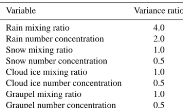
Table 1. The prescribed ratio (Vi) between the within-precipitation
variance and the mean squared of hydrometeors. Below-cloud val-ues are the same valval-ues as used for cloudy levels.
Variable Variance ratio
Rain mixing ratio 4.0
Rain number concentration 2.0
Snow mixing ratio 1.0
Snow number concentration 0.5
Cloud ice mixing ratio 1.0
Cloud ice number concentration 0.5
Graupel mixing ratio 1.0
Graupel number concentration 0.5
whereVi is the prescribed constant ratio between the vari-ance and the mean squared of each variate. Values forViused in the single-column simulations are provided in Table 1.
For multivariate PDFs, correlations among hydrometeor species must also be provided. In these simulations, the cor-relations are assumed to be constant within cloud through-out the course of the simulations. In order to assign val-ues for these correlations, we examined the range of valval-ues found within cloud-resolving model simulations (which vary in space and time), and prescribed correlations that were rep-resentative. The correlations used for cloudy levels are shown in Table 2. As with the variances, the correlations are within-hydrometeor values. In future work, instead of prescribing correlations, one could attempt to diagnose correlations, fol-lowing, e.g., Larson et al. (2011).
2.2.2 Incorporating the effects of latent heating of ice and rain on subgrid turbulence
Turbulence kinetic energy and turbulent fluxes of heat and moisture are influenced by the buoyancy of air parcels in local updrafts and downdrafts. The buoyancy variable in CLUBB is the virtual potential temperatureθv, whereθv in-cludes the effects on buoyancy of water vapor and cloud droplet loading. In CLUBB, buoyancy affects turbulence through four buoyancy generation terms that appear on the right-hand side of prognostic equations for moments (see Eqs. A5, A9, A10, A11). Ifg/θ0denotes the acceleration due to gravity divided by a constant reference temperature, then (g/θ0)w0θv0 is a buoyancy term that generates (that is, con-tributes to the tendency of)w02,(g/θ
0)w02θv0 generatesw03, (g/θ0)θl0θv0 generates w0θl0, and (g/θ0)r
0
tθv0 generates w0rt0. These buoyancy terms, in turn, are influenced by latent heat-ing associated with phase change of hydrometeors and grav-itational loading due to hydrometeors.
In prior versions of CLUBB, the only source of latent heating for the higher-order moments was condensation and evaporation of liquid cloud droplets, and the only source of loading was cloud liquid water mixing ratio. In other words, in the aforementioned four generation terms, the buoyancy
perturbationθv0 accounted only for variability due to the la-tent heating and water loading associated with cloud liquid water mixing ratio. (However, grid-mean values ofθlin prior versions of CLUBB were subject to the latent heating associ-ated with rain and ice hydrometeors, where relevant, through microphysical calculations.)
For the present simulations, we have incorporated a crude method to account for the latent heating and water loading associated with rain and ice hydrometeors in the four afore-mentioned buoyancy generation terms. Namely, we assume that for the purpose of calculating the four buoyancy gener-ation terms, rain and all ice hydrometeors are assumed to be perfectly collocated in space with cloud liquid water mixing ratio. With this simple assumption, CLUBB’s calculation of the four buoyancy generation terms remains unchanged, ex-cept that total condensate – including cloud liquid water, rain and ice mixing ratios – is input into the calculation in place of cloud liquid water. Conservation of heat and moisture for grid means still holds because this change only applies to the buoyancy generation terms. In the future, however, it would be desirable to examine the effects of this assumption. 2.2.3 Parameterizing transport of hydrometeors Turbulent updrafts and downdrafts transport hydrometeors in the vertical, thereby acting to broaden the vertical extent of the hydrometeor profiles. In CLUBB, the tendency of tur-bulence to broaden the hydrometeor profiles is modeled by eddy diffusion. Although it is not obvious a priori that an eddy diffusion model is appropriate for cumulus layers, our large-eddy simulations indicate that eddy diffusion parame-terizes the sign of hydrometeor transport satisfactorily in cu-mulus layers, but that the magnitude of the eddy diffusion is 1 or 2 orders of magnitude larger in cumulus than in stratocu-mulus layers (not shown).
CLUBB models the transport of a generic hydrometeor, rx, as
w0r0
x= −cK ∂rx
∂z, (2)
wherewdenotes the vertical velocity,c=0.75 a dimension-less constant, andzthe altitude. The eddy diffusivity for hy-drometeors,K, is given by
K= √
eL
q
r0
x2 rx
(1+ |Skw|) , (3)
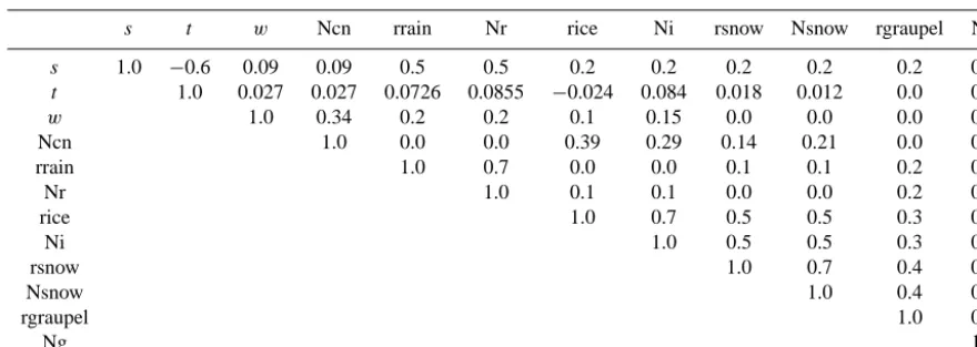
Table 2. Hydrometeor correlations used for all five cases. The variables included in the correlation matrix are, from left to right or top to bottom: extended liquid water mixing ratio, orthogonal extended liquid water mixing ratio, vertical velocity, extended cloud drop number concentration, and the mixing ratios and number concentrations of rain, cloud ice, snow, and graupel. Shown are the within-cloud values. For below cloud another correlation table is used, and for our purposes it is identical except for the correlation betweensandt. This correlation is set to 0.3 below cloud. The correlation matrix is symmetric, so the values below the diagonal are not filled in.
s t w Ncn rrain Nr rice Ni rsnow Nsnow rgraupel Ng
s 1.0 −0.6 0.09 0.09 0.5 0.5 0.2 0.2 0.2 0.2 0.2 0.0
t 1.0 0.027 0.027 0.0726 0.0855 −0.024 0.084 0.018 0.012 0.0 0.0
w 1.0 0.34 0.2 0.2 0.1 0.15 0.0 0.0 0.0 0.0
Ncn 1.0 0.0 0.0 0.39 0.29 0.14 0.21 0.0 0.0
rrain 1.0 0.7 0.0 0.0 0.1 0.1 0.2 0.0
Nr 1.0 0.1 0.1 0.0 0.0 0.2 0.0
rice 1.0 0.7 0.5 0.5 0.3 0.0
Ni 1.0 0.5 0.5 0.3 0.0
rsnow 1.0 0.7 0.4 0.0
Nsnow 1.0 0.4 0.0
rgraupel 1.0 0.0
Ng 1.0
2.2.4 Allowing microphysical sources to influence subgrid distribution shape
Microphysical processes influence not only grid box means, but also the shape of the subgrid PDF. For instance, micro-physical processes such as autoconversion and accretion oc-cur preferentially in moister portions of a grid box. Such pro-cesses, in conjunction with sedimentation of precipitation, tend to remove moisture from the moistest part of a grid box, thereby diminishing the variance of total water in cloud lay-ers (Khairoutdinov and Randall, 2002). In addition, evapo-ration of rain below cloud may at times occur in the coolest part of a grid box, thereby increasing variance of temperature below cloud. The increased subcloud temperature variance may, in principle, help initiate further convection.
These effects are estimated using SILHS subcolumns. Each subcolumn is fed into the microphysics separately, and each produces a separate microphysical update tortandθl. Therefore, the sample variance among the set of subcolumns is different before and after the microphysics is computed. This change in variance can be added as a source term in CLUBB’s prognostic equation for the scalar variance ofrtor θl. A similar calculation is made for the scalar fluxes ofrtand θl.
For a generic variablex, SILHS estimates the microphys-ical source as
∂x02 ∂t
!
microphys
≈ Var(x)|after−Var(x)|before
1t , (4)
where Var(x)is the sample variance ofxamong subcolumns, which is calculated before and after the call to the micro-physics, t denotes time, and1t is the time between
micro-physics calculations. Here,
Var(x)=
n
X
i=1
pi(xi−x)2, (5)
wheren is the number of subcolumns,xi is the value of x in theith subcolumn,x is the average over all subcolumns, andpiis the probability of choosing subcolumni. The prob-abilitypi equals 1/n in the case of equally weighted sub-columns, and the probability weights must sum to 1. An anal-ogous calculation is performed in order to update covariances between two variates.
In our simulations, the following prognostic moments are updated by microphysical source terms:rt02,θl02,rt0θl0,w0r0
t, andw0θ0
l. The prognostic equations for moments that involve onlyw, such asw02andw03, do not contain microphysical source terms, even in theory.
2.3 Model configurations and case descriptions
The following analysis compares two models, a single-column model (CLUBB-SILHS), and a 3-D cloud-resolving/large-eddy model (SAM; Khairoutdinov and Ran-dall, 2003) that provides reference simulations.
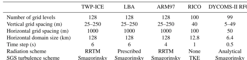
wa-Table 3. Options for SAM simulations of the five cases.
TWP-ICE LBA ARM97 RICO DYCOMS-II RF02
Number of grid levels 128 128 128 100 99
Vertical grid spacing (m) 25–250 25–250 25–250 40 5–49
Horizontal grid spacing (m) 1000 1000 1000 100 50
Horizontal domain size (km) 128 128 128 12.8 6.4
Time step (s) 6 6 4 1 0.5
Radiation scheme RRTM Prescribed RRTM None Analytical
SGS turbulence scheme Smagorinsky Smagorinsky Smagorinsky TKE Smagorinsky
ter, rain, cloud ice, snow, and graupel (Morrison et al., 2009). SILHS generates 16 sample subcolumns per time step.
We compare each CLUBB-SILHS single-column simula-tion with a three-dimensional simulasimula-tion performed by SAM. In order to help isolate model errors in CLUBB-SILHS, we configure SAM and CLUBB-SILHS identically in a number of aspects. Namely, SAM uses the same two-moment micro-physics scheme, the same value of prescribed within-cloud cloud droplet number concentration, and the same treatment of radiative transfer. SAM is set up similarly in shallow and deep cases, except that SAM uses smaller grid spacing and time step for the shallow cases. More SAM options for all cases are described below in Table 3.
2.3.1 Deep convective cases
We choose to simulate three deep convective cases that have been studied in prior model intercomparisons, in part because doing so allows us to compare our 3-D simulations with those intercomparison results, building confidence in our 3-D sim-ulations. We configure the deep convective simulations as per previous model intercomparisons of those cases. SAM sim-ulations examined here are comparable to previous simula-tions and observasimula-tions in general characteristics such as tim-ing, precipitation, and liquid water path. We conclude, there-fore, that they provide good reference simulations for eval-uation of CLUBB-SILHS. For deep convective cases, both SAM and CLUBB-SILHS prescribe droplet number concen-tration to be 100 cm−3, and both use the same 128-level ver-tical grid. SAM uses 1 km grid spacing in the horizontal.
The first deep convective case we present is from the Trop-ical Warm Pool International Cloud Experiment (TWP-ICE), which took place near Darwin, Australia, in early 2006 (May et al., 2008). The TWP-ICE case is a week-long simulation, beginning on 19 January and exhibiting multiple diurnal cy-cles of convective activity. Large-scale conditions are set up for the SAM and CLUBB simulations as in previous model intercomparison studies (Fridlind et al., 2012; Davies et al., 2013). Radiation in the SAM simulation is calculated by the Rapid Radiation Transfer Model (RRTM) (Iacono et al., 2008), and radiative heating values from SAM output are used to prescribe radiation in CLUBB-SILHS.
Figure 1. Time series of liquid water path (upper left), rain water path (upper right), ice water path (lower left), and snow water path (lower right) from the TWP-ICE deep convective simulation. Liquid water path is too high in the CLUBB-SILHS simulation, suggesting a low precipitation efficiency; however, the other hydrometeors fol-low SAM fairly closely.
The second case was taken from the Tropical Rain-fall Measuring Mission Large-Scale Biosphere-Atmosphere (TRMM-LBA) experiment which took place in Brazil in early 1999 (Silva Dias et al., 2002). The LBA case occurred on 23 February, and consists of the transition from shallow to deep convection over land from early morning to early af-ternoon. Model configurations for SAM and CLUBB-SILHS follow a previous model intercomparison (Grabowski et al., 2006; Khairoutdinov and Randall, 2006). In this case, both SAM and CLUBB-SILHS use prescribed radiation, as spec-ified in the intercomparison.
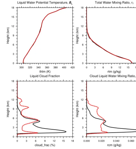
Figure 2. Profiles of liquid water potential temperature (θl) (upper left), total water mixing ratio (rt) (vapor+liquid) (upper right), liq-uid cloud fraction (lower left), and cloud liqliq-uid water mixing ratio (lower right) from the TWP-ICE deep convective simulation. Pro-files are averaged over minutes 6000–8000, capturing the strongest convective event. CLUBB-SILHS matches SAM well, with some small differences notable inθland liquid cloud fraction.
(ARM) program (ARM97). ARM97 is a 4-day simulation starting on 26 June that exhibits two weak precipitating con-vective events followed by a strong concon-vective event. We configure the case as in a previous intercomparison (Xu et al., 2002; Khairoutdinov and Randall, 2003). As in TWP-ICE, SAM uses RRTM to compute radiation, and SAM output is used to prescribe radiation in the CLUBB-SILHS simulation. 2.3.2 Shallow cloud-layer cases
The shallow cases are configured as in previous intercompar-ison studies, including the appropriate options for radiation and cloud drop number concentration. The vertical grid spac-ing and time step for CLUBB-SILHS are identical to that used for the deep convective cases. SAM’s configuration is summarized in Table 3.
The first shallow case we present is a 3-day simulation of drizzling trade-wind cumulus clouds observed during the Rain in shallow Cumulus over the Ocean (RICO) field cam-paign (Rauber et al., 2007). We configure RICO as in the intercomparison of vanZanten et al. (2011). As per the inter-comparison specifications, we prescribe a cloud drop number concentration of 70 cm−3in both CLUBB-SILHS and SAM, and radiation is turned off in both models.
Figure 3. Profiles of rain water mixing ratio (upper left), cloud ice mixing ratio (upper right), snow mixing ratio (lower left), and grau-pel mixing ratio (lower right) from the TWP-ICE deep convective simulation, averaged over the same time period as Fig. 2 (minutes 6000–8000). CLUBB-SILHS hydrometeor profiles match well with those simulated in SAM.
The second shallow case was taken from the Dynamics and Chemistry of Marine Stratocumulus (DYCOMS-II) field campaign (Stevens et al., 2003). We simulate the research flight 2 (RF02) case, which is a 6 h simulation of a noctur-nal drizzling stratocumulus layer off the coast of California (Wyant et al., 2007). DYCOMS-II RF02 uses a cloud drop number concentration of 55 cm−3 in both CLUBB-SILHS and SAM simulations (Ackerman et al., 2009). Both models use a simplified analytic radiation model which ties radiative heating to the liquid water path (Stevens et al., 2005; Wyant et al., 2007; Larson et al., 2007).
3 Results: simulated time series and profiles
liq-Figure 4. Time series of liquid water path (upper left), rain water path (upper right), ice water path (lower left), and snow water path (lower right) from the LBA deep convective simulation. Rain forms too late in the CLUBB-SILHS simulation, as there is an excess of ice that is not growing fast enough to form precipitation sized par-ticles; however, the timing and magnitude of liquid water path is simulated adequately.
uid water) (rt), the fraction of a grid box that is occupied by liquid cloud water, and cloud liquid water mixing ratio (rc).
3.1 Tropical deep convection: TWP-ICE
Time series of the four vertically integrated quantities from the TWP-ICE simulation are shown in Fig. 1. This was a convectively active period, and a strong diurnal signal can be seen in the time series. Because TWP-ICE is a tropical case, rainfall rate at the surface is constrained by prescribed large-scale forcings. Instead, we show rain water path. Rain water path simulated by CLUBB-SILHS mimics that in SAM, as does snow water path. LWP in CLUBB-SILHS is too high compared to SAM, while cloud ice is too low, which may mean that the correlations between liquid and ice hydrome-teors are not well tuned.
Figure 2 depicts four profiles averaged over the heaviest precipitation event, which occurs during minutes 6000–8000. In this case, CLUBB-SILHS agrees well with SAM and ex-hibits only a few discrepancies. Liquid water potential tem-perature (θl) is slightly too cool in the mid and upper levels, and the liquid cloud fraction is slightly too large in the lower levels. Figure 3 shows mean profiles of the mixing ratios of hydrometeors, again averaged over the strongest convective episode. All of CLUBB-SILHS’s profiles reproduce the cor-responding SAM profiles results well.
Figure 5. Profiles of liquid water potential temperature (θl) (upper left), total water mixing ratio (rt) (vapor+liquid) (upper right), liq-uid cloud fraction (lower left), and cloud liqliq-uid water mixing ratio (lower right) from the LBA deep convective simulation. Profiles are averaged over the last hour of the simulation (minutes 301–360). The CLUBB-SILHS simulation matches the CRM simulation well, aside from a lack of cloud in lower levels.
3.2 Transition from shallow to deep convection: LBA LBA is a difficult case to simulate because it evolves sub-stantially over a short (6 h) time period as it transitions from shallow to deep convection. Hence it is a challenge to sim-ulate the timing of ice and precipitation formation. Time se-ries from LBA are shown in Fig. 4. LWP in CLUBB-SILHS matches that in SAM well until the last hour of simulation time. In the last hour, LWP is depleted too much because rain forms more than an hour too late, and when it does form it produces excessive rain water path. The rain is delayed because precipitation efficiency is too low during the early period of weak forcing, possibly because of an inaccurate representation of the correlations among hydrometeors. The simulation overestimates cloud ice water path because the simulation produces too much cloud liquid aloft (Fig. 5).
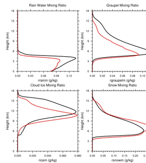
Figure 6. Profiles of rain water mixing ratio (upper left), cloud ice mixing ratio (upper right), snow mixing ratio (lower left), and grau-pel mixing ratio (lower right) from the LBA deep convective simu-lation, averaged over the same time period as Fig. 5 (minutes 301– 360). Profiles are consistent with what was seen in Fig. 4.
Cloud ice is overpredicted because the excess liquid aloft leads to large rates of contact nucleation (not shown). The large numbers of nucleated ice crystals also lead to decreased snow production from autoconversion due to the smaller crystal sizes.
3.3 Midlatitude continental convection: ARM97 Time series plots for ARM97 are shown in Fig. 7. The timing and magnitude of LWP is reasonably captured in SILHS. In the first convective event, however, CLUBB-SILHS’s cloud does not grow deep enough for the produc-tion of ice, and little rain is produced. The later convective episodes are better simulated, although CLUBB-SILHS’s time series are too noisy.
Mean profiles for ARM97 are shown in Fig. 8, averaged over the third and strongest convective event (minutes 4320– 5580). Similar to what was seen in TWP-ICE,θlin CLUBB-SILHS is too cool aloft, andrtand liquid cloud fraction are too large through the lowest 6–7 km of the column. Hydrom-eteor profiles (Fig. 9) match fairly well to the SAM CRM (cloud resolving model) simulation, though CLUBB-SILHS does not produce enough ice aloft. The undesirably low pre-cipitation efficiency seen in TWP-ICE is also evident in this case, as too much liquid is needed to produce the correct amount of rain.
Figure 7. Time series of liquid water path (upper left), rain ter path (upper right), ice water path (lower left), and snow wa-ter path (lower right) from the ARM97 deep convective simulation. CLUBB-SILHS’s simulation of the first event produces cloud liquid water but no precipitation. However, CLUBB-SILHS’s simulation of the other two events match SAM well in timing and magnitude.
3.4 Examining the representation of dynamics
Figure 8. Profiles of liquid water potential temperature (upper left), total water mixing ratio (vapor+liquid) (upper right), liq-uid cloud fraction (lower left), and cloud liqliq-uid water mixing ratio (lower right) from the ARM97 deep convective simulation. Profiles are averaged over the third convective event (minutes 4321–5580). CLUBB-SILHS is slightly too cool in the upper troposphere and too moist in the lower troposphere; liquid cloud fraction is too large.
4 Effects of our new methodology on deep convective simulations
Two of the changes to CLUBB described in Sect. 2.2 have significant effects on the simulation of deep convection.
First, improving the PDF for hydrometeors by including a nonunity precipitation fraction (Sect. 2.2.1) – that is, al-lowing a region free of hydrometeors (cloud ice, snow, grau-pel, and rain) – improved LBA (Fig. 11). With the pre-vious formulation, liquid cloud water increases to overly large values by the end of the simulation, and the excessive cloud water nucleates to form excessive cloud ice. However, no rain forms during the 6 h simulation. The addition of a hydrometeor-free region improves (increases) the precipita-tion efficiency of CLUBB-SILHS, allowing rain to form and remove excessive liquid cloud water.
Second, it turns out to be important for the simulations of deep convective cases to have strong turbulent transport of hydrometeors. The changes introduced to the eddy diffusiv-ity calculation in Sect. 2.2.3 allow for stronger values in con-vective cases (while not degrading shallow cases, as shown in Sect. 6). Larger values of eddy diffusivity smooth the profiles of hydrometeors and transport hydrometeors farther upward, leading to closer agreement with SAM (see Fig. 12).
Figure 9. Profiles of rain water mixing ratio (upper left), cloud ice mixing ratio (upper right), snow mixing ratio (lower left), and grau-pel mixing ratio (lower right) from the ARM97 deep convective simulation, average over the same time as Fig. 8 (minutes 4321– 5580). The hydrometeor profiles match the CRM fairly well, though the ice hydrometeors are too few and do not reach high enough in the clouds.
The other two methodological changes – adding latent heating to subgrid moments (Sect. 2.2.2) and adding micro-physical source terms to prognosed second-order moments (Sect. 2.2.4) – have more minor effects on the simulations.
5 Sensitivity to time step, number of samples, and vertical grid spacing
Aside from the errors explicitly mentioned above, the CLUBB-SILHS results presented here agree well with SAM. However, the configuration of CLUBB-SILHS used – with its fine vertical resolution, short time step, and numerous sample points – is computationally expensive. In this sec-tion, we present results that use configurations that are more computationally affordable.
Figure 10. CLUBB-SILHS simulations of TWP-ICE (above), LBA (middle), and ARM97 (below) demonstrating the ability of CLUBB-SILHS to simulate dynamics for the deep convective cases. For each case, the variance of vertical velocity is shown on the left, the turbulent flux of liquid water potential temperature is in the middle, and the turbulent flux of total water mixing ratio is on the right (averaged over the same time periods as in previous figures). CLUBB-SILHS matches the CRM well in variance of vertical ve-locity, but underestimates the magnitude of some of the turbulent fluxes, particularly in the more convectively active cases.
fraction aloft. This may be partly related to an underpredic-tion of subcloud evaporative cooling that occurs when prog-nostic microphysics schemes with sequential time splitting of sedimentation allow hydrometeors to sediment long dis-tances between calls to the microphysical sources and sinks, such as evaporation (H. Morrison, personal communication, March 2014).
It is possible to use CLUBB-SILHS with any (even) num-ber of subcolumns. Using more subcolumns leads to better sampling and hence more accurate estimates of averages of SGS variability (Larson and Schanen, 2013). However, feed-ing fewer subcolumns into the microphysics scheme reduces computational cost. We have presented results using 16 sub-columns, which is a compromise between accuracy and com-putational cost. Shown in Fig. 14 are the results of reducing the number of sample columns from 16 to 4. The results are similar, with the exception of LBA, which, with four sample points, does not produce surface precipitation, thereby per-mitting large amounts of cloud water to remain aloft.
Computational cost can also be reduced by coarsening the vertical resolution. To test the effects of this, Fig. 15 plots
Figure 11. LBA simulations showing the sensitivity to the inclusion of the new precipitation fraction. The black line is the SAM CRM simulation, the red dashed line is the CLUBB-SILHS (default) sim-ulation presented in Sect. 3.2, which includes the precipitation frac-tion, and the blue dotted line is CLUBB-SILHS with the same con-figuration as in the red line, but with the option for the precipitation fraction set to false. Above are profiles of cloud liquid water mixing ratio (left) and cloud ice mixing ratio (right), averaged over the last hour of the simulation (minutes 301–360). Below are time series of liquid water path (left) and rain water path (right). Nonzero precipi-tation fraction is important for LBA, because it increases precipita-tion efficiency, allowing more rain to leave the atmosphere, thereby removing excess cloud liquid water aloft and reducing excessive ice formation and growth.
simulations of the deep convective cases, configured identi-cally as before except that they use the 30-level stretched grid that is used in the CAM climate model (Neale et al., 2012). The simulations are adequate, but they are too convectively active and contain too much condensate. This is particularly apparent in LBA, which again has excessive cloud water aloft because the precipitation efficiency is too low.
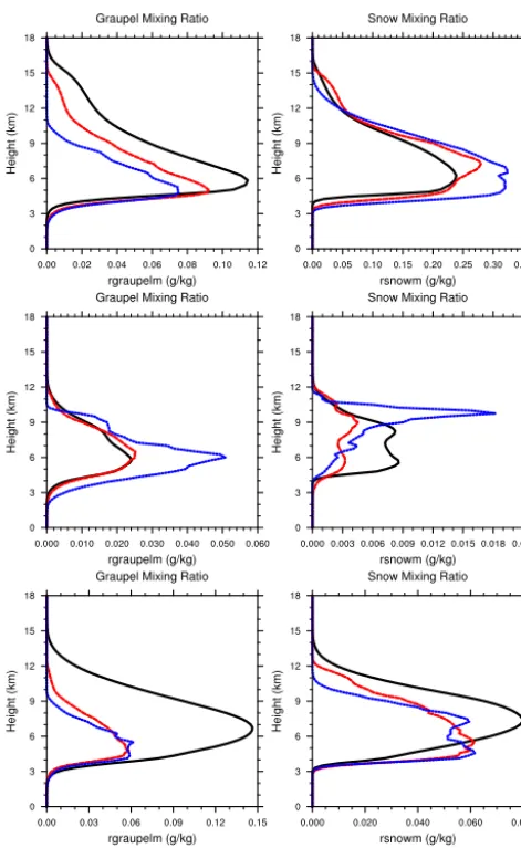
Figure 12. TWP-ICE (above), LBA (middle), and ARM97 (below) simulations showing the sensitivity to the boosted eddy diffusivity for convective cases. For each case, graupel mixing ratio is shown on the left and snow mixing ratio on the right. The black line is the SAM CRM simulation, the red dashed line is the CLUBB-SILHS simulation configured exactly as that presented earlier in Sect. 3, and the blue dotted line is CLUBB-SILHS with the same configu-ration as in the red line, but without the new diffusivity calculation. The new formulation for eddy diffusivity smooths the hydrometeor profiles and transports hydrometeors farther aloft.
6 How does the generalized coupling to microphysics influence shallow cloud simulations?
Using the same configuration as used for the deep convective cases, we also simulate two shallow cloud cases. We find that these two cases are not degraded by the modifications intro-duced into CLUBB-SILHS in order to improve deep convec-tive simulations.
Results from the RICO shallow cumulus case are shown in Fig. 16. CLUBB-SILHS simulates this trade-wind cumu-lus case reasonably well, although CLUBB-SILHS
underes-Figure 13. CLUBB-SILHS simulations of TWP-ICE (above), LBA (middle), and ARM97 (below) showing sensitivity of simulations to the time step. For each case, liquid cloud fraction is shown on the left (averaged over the same time periods as in previous figures) and a time series of snow water path is shown on the right. The black line is the SAM CRM simulation, the red dashed line is the (de-fault) CLUBB-SILHS simulation presented earlier in Sect. 3, and the blue dotted line is CLUBB-SILHS with the same configuration as in the red line, but using a 5 min time step, rather than 1 min. With an increased time step, the CLUBB-SILHS simulations are too con-vectively active; however, the simulations are still reasonable when compared to the SAM CRM simulations.
timates cloud liquid water. However, the underestimate is not introduced by the modifications to CLUBB-SILHS. Rather, these errors are typical of some prior versions of CLUBB.
Figure 14. CLUBB-SILHS simulations of TWP-ICE (above), LBA (middle), and ARM97 (below) showing sensitivity of simulations to the number of subcolumns utilized in SILHS. For each case, liquid cloud fraction is shown on the left (averaged over the same time pe-riods as in previous figures) and a time series of snow water path is shown on the right. The black line is the SAM CRM simulation, the red dashed line is the CLUBB-SILHS simulation presented earlier in Sect. 3, and the blue dotted line is CLUBB-SILHS with the same configuration as in the red line, but using only four subcolumns for SILHS, rather than 16. Results are degraded only slightly with a re-duced number of subcolumns, except in the LBA case, where too much cloud forms aloft.
the lowest 1200 m of the domain. At higher resolutions, CLUBB-SILHS simulates greater liquid water content for the DYCOMS-II RF02 case (Griffin and Larson, 2013).
Although further study is necessary, the fact that reason-able results can be obtained for shallow convection with the same model configuration as for deep convection hints that a unified PDF parameterization may indeed be possible, with one equation set representing all turbulence and cloud types.
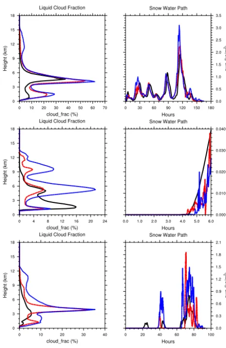
Figure 15. CLUBB-SILHS simulations of TWP-ICE (above), LBA (middle), and ARM97 (below) showing sensitivity of simulations to the number of vertical grid levels. For each case, liquid cloud fraction is shown on the left (averaged over the same time periods as in previous figures) and a time series of snow water path is shown on the right. The black line is the SAM CRM simulation, the red dashed line is the (default) CLUBB-SILHS simulation presented in Sect. 3, and the blue dotted line is CLUBB-SILHS with the same configuration as in the red line, but using a 30-level vertical grid, rather than a 128-level grid. The CLUBB-SILHS simulations with decreased vertical resolution contain too much condensate, which is particularly apparent in the LBA case.
7 Conclusions
Figure 16. Results from the RICO simulation of shallow cumu-lus clouds. Above are time series of liquid water path (upper left) and rain water path (upper right). Below are mean profiles of liq-uid water potential temperature (middle left), total water mixing ratio (middle right), liquid cloud fraction (lower left), and cloud liquid water mixing ratio (lower right). Profiles are averaged over the last 2 h of the simulation (minutes 4301–4320). The CLUBB-SILHS simulation looks comparable to SAM, though there is too little cloud water produced.
important for deep convection, which has strong interactions between dynamics and microphysics.
Most of the simulated fields are satisfactory, although there exist a few deficiencies. One is that rain forms 100 min too late in the LBA case of transition from shallow to deep convection (see Fig. 4). Another deficiency is that pre-cipitation does not form in the first of the three convec-tive events in ARM97 (see Fig. 7). Both these deficiencies suggest that CLUBB-SILHS produces insufficient precipita-tion when convecprecipita-tion is weakly forced. Furthermore, when CLUBB-SILHS’s time step is degraded to 5 min (see Fig. 13) or the number of vertical grid levels is degraded to 30 (see Fig. 15), the simulated updrafts are too strong, the surface
Figure 17. Results from the DYCOMS-II RF02 simulation of stra-tocumulus clouds. Above are time series of liquid water path (upper left) and rain water path (upper right). Below are mean profiles of liquid water potential temperature (middle left), total water mix-ing ratio (middle right), liquid cloud fraction (lower left), and cloud liquid water mixing ratio (lower right). Profiles are averaged over the last hour of the simulation (minutes 301–360). CLUBB-SILHS does a reasonable job of simulating these shallow stratocumulus clouds, though the amount of liquid is too low, which is related to the coarse vertical grid spacing.
precipitation is too weak, and too much cloud forms aloft. Again, these are symptoms of low precipitation efficiency. That is, the amount of precipitation produced in CLUBB-SILHS for an amount of condensate is too low in these cases – leaving too much cloud water remaining compared to the SAM simulations.
to simulate deep convection? One is CLUBB-SILHS’s de-tailed representation of and coupling between turbulence and microphysics and, in particular, ice microphysics. CLUBB-SILHS uses a delta–lognormal subgrid PDF of hydromete-ors, which allows for the possibility of a hydrometeor-free region of a grid box and also allows the hydrometeors to fall preferentially through liquid cloud water. This, in turn, al-lows more precipitation to reach the ground, reducing cloud water aloft (see Fig. 11). Although the precipitation effi-ciency is still somewhat too low in the simulations, the delta– lognormal PDF does improve precipitation efficiency. An-other key ingredient is vertical turbulent transport of hydrom-eteors, which increases the altitude reached by snow and other hydrometeors.
Appendix A: CLUBB equations
CLUBB includes predictive equations for the horizontal winds (uandv), total waterrt (liquid+vapor), liquid water potential temperatureθl, and several higher-order moments. The following are the prognostic equations in the CLUBB model, provided for reference:
∂u¯
∂t = − ¯w
∂u¯
∂z−f (vg− ¯v)− 1 ρs
∂ρsu0w0
∂z +
∂u¯
∂t ls , (A1)
∂v¯
∂t = − ¯w
∂v¯
∂z+f (ug− ¯u)− 1 ρs
∂ρsv0w0
∂z +
∂v¯
∂t ls , (A2)
∂r¯t
∂t = − ¯w
∂r¯t ∂z −
1 ρs
∂ρsw0rt0
∂z +
∂r¯t ∂t ls , (A3)
∂θ¯l
∂t = − ¯w
∂θ¯l ∂z −
1 ρs
∂ρsw0θl0 ∂z + ¯R+
∂θ¯l ∂t ls , (A4)
∂w02
∂t = − ¯w
∂w02 ∂z −
1 ρs
∂ρsw03 ∂z −2w
02∂w¯ ∂z +
2g θvs
w0θ0 v (A5)
−C4
τ
w02−2 3e¯
−C5
−2w02∂w¯ ∂z +
2g θvs
w0θ0 v
+2
3C5
g
θvs w0θ0
v−u0w0 ∂u¯
∂z−v
0w0∂v¯
∂z
−C1
τ
w02−w|2 tol
+ ∂
∂z
(Kw1+ν1) ∂ ∂zw
02
,
∂rt02
∂t = − ¯w
∂rt02 ∂z −
1 ρs
∂ρsw0rt02
∂z −2w
0r0 t
∂r¯t
∂z (A6)
−C2
τ
rt02−rt|2tol
+ ∂
∂z
(Kw2+ν2) ∂ ∂zr 02 t ,
∂θl02
∂t = − ¯w
∂θl02 ∂z −
1 ρs
∂ρsw0θl02
∂z −2w
0θ0 l
∂θ¯l
∂z (A7)
−C2
τ
θl02−θl|2tol
+ ∂
∂z
(Kw2+ν2) ∂ ∂zθ 02 l ,
∂rt0θl0
∂t = − ¯w
∂rt0θl0 ∂z −
1 ρs
∂ρsw0rt0θl0
∂z −w
0r0 t
∂θ¯l
∂z (A8)
−w0θ0 l
∂r¯t ∂z−
C2 τ r
0 tθl0+
∂ ∂z
(Kw2+ν2) ∂ ∂zr
0 tθl0
,
∂w0r0 t
∂t = − ¯w
∂w0r0 t ∂z −
1 ρs
∂ρsw02rt0
∂z −w
02∂r¯t
∂z (A9)
−w0r0 t
∂w¯
∂z + g
θvs rt0θ0
v− C6
τ w
0r0
t+C7w0rt0 ∂w¯
∂z
−C7
g θvs
rt0θv0+ ∂ ∂z
(Kw6+ν6) ∂ ∂zw
0r0 t
,
∂w0θ0 l
∂t = − ¯w
∂w0θ0 l ∂z −
1 ρs
∂ρsw02θl0
∂z −w
02∂θ¯l
∂z (A10)
−w0θ0 l
∂w¯
∂z + g θvs
θl0θ0 v−
C6 τ w
0θ0 l+C7w
0θ0 l
∂w¯
∂z
−C7
g
θvs θl0θ0
v+ ∂
∂z
(Kw6+ν6) ∂
∂zw
0θ0 l
,
∂w03
∂t = − ¯w
∂w03 ∂z −
1 ρs
∂ρsw04 ∂z +3
w02 ρs
∂ρsw02
∂z (A11)
−3w03∂w¯ ∂z +
3g θvs
w02θ0 v
−C15Km
g θvs
∂w0θ0 v ∂z −
∂u0w0∂u¯
z
∂z +
∂v0w0∂v¯
z ∂z
−C8
τ w
03−C 11
−3w03∂w¯ ∂z +
3g θvs
w02θ0 v
+ ∂
∂z
(Kw8+ν8) ∂ ∂zw
03
,
Acknowledgements. Coauthors from the University of Wisconsin– Milwaukee acknowledge support by the Office of Science, US Department of Energy, under grants DE-SC0008668 (BER) and DE-SC0008323 (Scientific Discoveries through Advanced Computing, SciDAC). P. Rasch was supported by SciDAC, and M. Wang was supported by SciDAC and the DOE Atmospheric System Research (ASR) Program. The Pacific Northwest National Laboratory is operated for DOE by Battelle Memorial Institute under contract DE-AC06-76RLO 1830. The authors would like to thank Mikhail Ovchinnikov and Steven Ghan for helpful discussions. In addition, the authors would like to thank the two anonymous reviewers who provided helpful comments which improved the original manuscript.
Edited by: R. Neale
References
Ackerman, A. S., van Zanten, M. C., Stevens, B., Savic-Jovcic, V., Bretherton, C. S., Chlond, A., Golaz, J.-C., Jiang, H., Khairout-dinov, M., Krueger, S. K., Lewellen, D. C., Lock, A., Moeng, C.-H., Nakamura, K., Petters, M. D., Snider, J. R., Weinbrecht, S., and Zulauf, M.: Large-Eddy Simulations of a Drizzling, Stratocumulus-Topped Marine Boundary Layer, Mon. Weather Rev., 137, 1083–1110, doi:10.1175/2008MWR2582.1, 2009. Arakawa, A.: The cumulus parameterization problem: Past, present,
and future, J. Climate, 17, 2493–2525, 2004.
Arakawa, A. and Schubert, W. H.: Interaction of a cumulus cloud ensemble with the large-scale environment, part I, J. Atmos. Sci., 31, 674–701, 1974.
Arakawa, A., Jung, J.-H., and Wu, C.-M.: Toward unification of the multiscale modeling of the atmosphere, Atmos. Chem. Phys., 11, 3731–3742, doi:10.5194/acp-11-3731-2011, 2011.
Bechtold, P., Semane, N., Lopez, P., Chaboureau, J.-P., Beljaars, A., and Bormann, N.: Representing Equilibrium and Nonequilibrium Convection in Large-Scale Models, J. Atmos. Sci., 71, 734–753, 2014.
Bogenschutz, P. A. and Krueger, S. K.: A simplified PDF param-eterization of subgrid-scale clouds and turbulence for cloud-resolving models, J. Adv. Model. Earth Syst., 5, 195–211, doi:10.1002/jame.20018, 2013.
Bogenschutz, P. A., Gettelman, A., Morrison, H., Larson, V. E., Schanen, D. P., Meyer, N. R., and Craig, C.: Unified parameter-ization of the planetary boundary layer and shallow convection with a higher-order turbulence closure in the Community Atmo-sphere Model: single-column experiments, Geosci. Model Dev., 5, 1407–1423, doi:10.5194/gmd-5-1407-2012, 2012.
Bogenschutz, P. A., Gettelman, A., Morrison, H., Larson, V. E., Craig, C., and Schanen, D. P.: Higher-Order Turbulence Closure and Its Impact on Climate Simulations in the Community Atmo-sphere Model, J. Climate, 26, 9655–9676, doi:10.1175/JCLI-D-13-00075.1, 2013.
Bony, S. and Emanuel, K. A.: A parameterization of the cloudiness associated with cumulus convection; Evaluation using TOGA COARE data, J. Atmos. Sci., 58, 3158–3183, 2001.
Cheng, A. and Xu, K.-M.: Simulation of shallow cumuli and their transition to deep convective clouds by cloud-resolving models
with different third-order turbulence closures, Q. J. Roy. Meteo-rol. Soc., 132, 359–382, 2006.
Davies, L., Jakob, C., Cheung, K., Genio, A. D., Hill, A., Hume, T., Keane, R. J., Komori, T., Larson, V. E., Lin, Y., Liu, X., Nielsen, B. J., Petch, J., Plant, R. S., Singh, M. S., Shi, X., Song, X., Wang, W., Whitall, M. A., Wolf, A., Xie, S., and Zhang, G.: A single-column model ensemble approach applied to the TWP-ICE experiment, J. Geophys. Res., 118, 6544–6563, doi:10.1002/jgrd.50450, 2013.
Donner, L. J.: A cumulus parameterization including mass fluxes, vertical momentum dynamics, and mesoscale effects, J. Atmos. Sci., 50, 889–906, 1993.
Fridlind, A. M., Ackerman, A. S., Chaboureau, J.-P., Fan, J., Grabowski, W. W., Hill, A. A., Jones, T. R., Khaiyer, M. M., Liu, G., Minnis, P., Morrison, H., Nguyen, L., Park, S., Petch, J. C., Pinty, J.-P., Schumacher, C., Shipway, B. J., Varble, A. C., Wu, X., Xie, S., and Zhang, M.: A comparison of TWP-ICE ob-servational data with cloud-resolving model results, J. Geophys. Res., 117, D05204, doi:10.1029/2011JD016595, 2012.
Gerard, L.: An integrated package for subgrid convection, clouds and precipitation compatible with meso-gamma scales, Q. J. Roy. Meteorol. Soc., 133, 711–730, 2007.
Gettelman, A. and Morrison, H.: Advanced Two-Moment Bulk Microphysics for Global Models. Part I: Off-Line Tests and Comparison with Other Schemes, J. Climate, online first, doi:10.1175/JCLI-D-14-00102.1, 2014.
Golaz, J.-C., Larson, V. E., and Cotton, W. R.: A PDF-based model for boundary layer clouds. Part I: Method and model description, J. Atmos. Sci., 59, 3540–3551, 2002.
Grabowski, W. W., Bechtold, P., Cheng, A., Forbes, R., Halliwell, C., Khairoutdinov, M., Lang, S., Nasuno, T., Petch, J., Tao, W. K., Wong, R., Wu, X., and Xu, K. M.: Daytime convective development over land: A model intercomparison based on LBA observations, Q. J. Roy. Meteorol. Soc., 132, 317–344, 2006. Griffin, B. M. and Larson, V. E.: Analytic upscaling of local
micro-physics parameterizations, Part II: Simulations, Q. J. Roy. Mete-orol. Soc., 139, 58–69, 2013.
Griffin, B. M. and Larson, V. E.: A multivariate subgrid probability density function for hydrometeors, Geosci. Model Dev. Discuss., in preparation, 2014.
Iacono, M. J., Delamere, J. S., Mlawer, E. J., Shephard, M. W., Clough, S. A., and Collins, W. D.: Radiative forcing by long-lived greenhouse gases: Calculations with the AER ra-diative transfer models, J. Geophys. Res., 113, D13103, doi:10.1029/2008JD009944, 2008.
Kain, J. S.: The Kain–Fritsch Convective Parameterization: An Up-date, J. Appl. Meteorol., 43, 170–181, 2004.
Kain, J. S. and Fritsch, J. M.: A one-dimensional entrain-ing/detraining plume model and its application in convective pa-rameterization, J. Atmos. Sci., 47, 2784–2802, 1990.
Khairoutdinov, M. and Randall, D. A.: Similarity of Deep Conti-nental Cumulus Convection as Revealed by a Three-Dimensional Cloud-Resolving Model, J. Atmos. Sci., 59, 2550–2566, 2002. Khairoutdinov, M. and Randall, D. A.: Cloud Resolving
Khairoutdinov, M. and Randall, D. A.: High-Resolution Simulation of Shallow-to-Deep Convection Transition over Land, J. Atmos. Sci., 63, 3421–3436, 2006.
Larson, V. E. and Golaz, J.-C.: Using probability density functions to derive consistent closure relationships among higher-order moments, Mon. Weather Rev., 133, 1023–1042, 2005.
Larson, V. E. and Griffin, B. M.: Analytic upscaling of local micro-physics parameterizations, Part I: Derivation, Q. J. Roy. Meteo-rol. Soc., 139, 46–57, 2013.
Larson, V. E. and Schanen, D. P.: The Subgrid Importance Latin Hy-percube Sampler (SILHS): a multivariate subcolumn generator, Geosci. Model Dev., 6, 1813–1829, doi:10.5194/gmd-6-1813-2013, 2013.
Larson, V. E., Wood, R., Field, P. R., Golaz, J.-C., Vonder Haar, T. H., and Cotton, W. R.: Small-scale and mesoscale variability of scalars in cloudy boundary layers: One-dimensional probabil-ity densprobabil-ity functions, J. Atmos. Sci., 58, 1978–1994, 2001. Larson, V. E., Golaz, J.-C., Jiang, H., and Cotton, W. R.: Supplying
Local Microphysics Parameterizations with Information about Subgrid Variability: Latin Hypercube Sampling, J. Atmos. Sci., 62, 4010–4026, 2005.
Larson, V. E., Kotenberg, K. E., and Wood, N. B.: An analytic long-wave radiation formula for liquid layer clouds, Mon. Weather Rev., 135, 689–699, 2007.
Larson, V. E., Nielsen, B. J., Fan, J., and Ovchinnikov, M.: Parameterizing correlations between hydrometeors in mixed-phase Arctic clouds, J. Geophys. Res., 116, D00T02, doi:10.1029/2010JD015570, 2011.
Larson, V. E., Schanen, D. P., Wang, M., Ovchinnikov, M., and Ghan, S.: PDF parameterization of boundary layer clouds in models with horizontal grid spacings from 2 to 16 km, Mon. Weather Rev., 140, 285–306, 2012.
Lewellen, W. S. and Yoh, S.: Binormal model of ensemble partial cloudiness, J. Atmos. Sci., 50, 1228–1237, 1993.
Liu, C., Moncrieff, M. W., and Zipser, E. J.: Dynamical influence of microphysics in tropical squall lines: a numerical study, Mon. Weather Rev., 125, 2193–2210, 1997.
Mapes, B. and Neale, R.: Parameterizing convective organization to escape the entrainment dilemma, J. Adv. Model. Earth Syst., 3, M06004, doi:10.1029/2011MS000042, 2011.
May, P. T., Mather, J. H., Vaughan, G., Bower, K. N., Jakob, C., Mc-Farquhar, G. M., and Mace, G. G.: The Tropical Warm Pool Inter-national Cloud Experiment, B. Am. Meteorol. Soc., 89, 629–645, 2008.
McKay, M. D., Beckman, R. J., and Conover, W. J.: A compari-son of three methods for selecting values of input variables in the analysis of output from a computer code, Technometrics, 21, 239–245, 1979.
Mellor, G. L.: The Gaussian cloud model relations, J. Atmos. Sci., 34, 356–358, 1977.
Molinari, J. and Dudek, P.: Parameterization of Convective Precipi-tation in Mesoscale Numerical Models: A Critical Review, Mon. Weather Rev., 120, 326–344, 1992.
Morrison, H. and Gettelman, A.: A New Two-Moment Bulk Strat-iform Cloud Microphysics Scheme in the Community Atmo-sphere Model, Version 3 (CAM3). Part I: Description and Nu-merical Tests, J. Climate., 21, 3642–3659, 2008.
Morrison, H., Thompson, G., and Tatarskii, V.: Impact of cloud mi-crophysics on the development of trailing stratiform precipitation
in a simulated squall line: Comparison of one- and two-moment schemes, Mon. Weather Rev., 137, 993–1009, 2009.
Neale, R. B., Gettelman, A., Park, S., Chen, C.-C., Lauritzen, P. H., Williamson, D. L., Conley, A. J., Kinnison, D., Marsh, D., Smith, A. K., Vitt, F., Garcia, R., Lamarque, J.-F., Mills, M., Tilmes, S., Morrison, H., Cameron-Smith, P., Collins, W. D., Iacono, M. J., Easter, R. C., Ghan, S. J., Liu, X., Rasch, P. J., and Taylor, M. A.: Description of the NCAR Community Atmosphere Model (CAM5.0), Tech. Rep. NCAR/TN-486+STR, National Center for Atmospheric Research, Boulder, CO, USA, 2012.
Noda, A. T., Oouchi, K., Satoh, M., Tomita, H., Iga, S.-I., and Tsushima, Y.: Importance of the subgrid-scale turbulent moist process: Cloud distribution in global cloud-resolving simula-tions, Atmos. Res., 96, 208–217, 2010.
Owen, A. B.: Quasi-Monte Carlo Techniques, in: Siggraph 2003, Course 44, San Diego, CA, Association for Computing Machin-ery, 2003.
Posselt, R. and Lohmann, U.: Sensitivity of the total anthropogenic aerosol effect to the treatment of rain in a global climate model, Geophys. Res. Lett., 36, L02805, doi:10.1029/2008GL035796, 2009.
Rauber, R. M., Stevens, B., Ochs, H. T., Knight, C., Albrecht, B. A., Blyth, A. M., Fairall, C. W., Jensen, J. B., Lasher-Trapp, S. G., Mayol-Bracero, O. L., Vali, G., Anderson, J. R., Baker, B. A., Bandy, A. R., Burnet, E., Brenguier, J.-L., Brewer, W. A., Brown, P. R. A., Chuang, P., Cotton, W. R., Girolamo, L. D., Geerts, B., Gerber, H., Göke, S., Gomes, L., Heikes, B. G., Hud-son, J. G., Kollias, P., LawHud-son, R. P., Krueger, S. K., Lenschow, D. H., Nuijens, L., O’Sullivan, D. W., Rilling, R. A., Rogers, D. C., Siebesma, A. P., Snodgrass, E., Stith, J. L., Thornton, D. C., Tucker, S., Twohy, C. H., Zuidema, P., Sperber, K. R., and Waliser, D. E.: Rain in Shallow Cumulus Over the Ocean: The RICO Campaign, B. Am. Meteorol. Soc., 88, 1912–1928, 2007. Reed, K. A., Jablonowski, C., and Taylor, M. A.: Tropical cyclones in the spectral element configuration of the Cimmunity Atmo-sphere Model, Atmos. Sci. Lett., 13, 303–310, 2012.
Sato, T., Miura, H., Satoh, M., Takayabu, Y. N., and Wang, Y.: Di-urnal cycle of precipitation in the tropics simulated in a global cloud-resolving model, J. Climate, 22, 4809–4826, 2009. Silva Dias, M. A. F., Rutledge, S., Kabat, P., Silva Dias, P. L.,
Nobre, C., Fisch, G., Dolman, A. J., Zipser, E., Garstang, M., Manzi, A. O., Fuentes, J. D., Rocha, H. R., Marengo, J., Plana-Fattori, A., Sá, L. D. A., Alvalá, R. C. S., Andreae, M. O., Ar-taxo, P., Gielow, R., and Gatti, L.: Cloud and rain processes in a biosphere-atmosphere interaction context in the Amazon region, J. Geophys. Res., 107, 8072, doi:10.1029/2001JD000335, 2002. Smith, R. N. B.: A scheme for predicting layer clouds and their water content in a general circulation model, Q. J. Roy. Meteorol. Soc., 116, 435–460, 1990.
Sommeria, G. and Deardorff, J. W.: Subgrid-scale condensation in models of nonprecipitating clouds, J. Atmos. Sci., 34, 344–355, 1977.
Zan-ten, M. C.: Dynamics and chemistry of marine stratocumulus – DYCOMS-II, B. Am. Meteorol. Soc., 84, 579–593, 2003. Stevens, B., Moeng, C.-H., Ackerman, A. S., Bretherton, C. S.,
Chlond, A., de Roode, S., Edwards, J., Golaz, J.-C., Jiang, H., Khairoutdinov, M., Kirkpatrick, M. P., Lewellen, D. C., Lock, A., Müller, F., Stevens, D. E., Whelan, E., and Zhu, P.: Evaluation of large-eddy simulations via observations of nocturnal marine stra-tocumulus, Mon. Weather Rev., 133, 1443–1462, 2005. Tompkins, A. M.: Organization of tropical convection in low
verti-cal wind shears: The role of cold pools, J. Atmos. Sci., 58, 1650– 1672, 2001.
Tompkins, A. M.: A prognostic parameterization for the subgrid-scale variability of water vapor and clouds in large-subgrid-scale models and its use to diagnose cloud cover, J. Atmos. Sci., 59, 1917– 1942, 2002.
vanZanten, M., Stevens, B., Nuijens, L., Siebesma, A., Ackerman, A., Burnet, F., Cheng, A., Couvreux, F., Jiang, H., Khairoutdinov, M., Kogan, Y., Lewellen, D., Mechem, D., Nakamura, K., Noda, A., Shipway, B., Slawinska, J., Wang, S., and Wyszogrodzki, A.: Controls on precipitation and cloudiness in simulations of trade-wind cumulus as observed during RICO, J. Adv. Model. Earth Syst., 3, M06001, doi:10.1029/2011MS000056, 2011.
Warner, T. T. and Hsu, H.-M.: Nested-Model Simulation of Moist Convection: The Impact of Coarse-Grid Parameterized Convec-tion on Fine-Grid Resolved ConvecConvec-tion, Mon. Weather Rev., 128, 2211–2231, 2000.
Wehner, M. F., Reed, K. A., Li, F., Prabhat, Bacmeister, J., Chen, C.-T., Paciorek, C., and Gleckler, P. J., Sperber, K. R., Collins, W. D., Gettelman, A., and Jablonowski, C.: The effect of hori-zontal resolution on simulation quality in the Community Atmo-sphere Model, CAM5.1, Journal of Advances in Modeling Earth Systems, online first, doi:10.1002/2013MS000276, 2014.
Weisman, M. L., Skamarock, W. C., and Klemp, J. B.: The Reso-lution Dependence of Explicitly Modeled Convective Systems, Mon. Weather Rev., 125, 527–548, 1997.
Williamson, D. L.: Dependence of APE simulations on vertical res-olution with the Cimmunity Atmosphere Model, version 3, J. Meteorol. Soc. Jpn., 91A, 231–242, 2013a.
Williamson, D. L.: The effect of time steps and time-scales on pa-rameterization suites, Q. J. Roy. Meteorol. Soc., 139, 548–560, 2013b.
Wyant, M. C., Bretherton, C. S., Chlond, A., Griffin, B. M., Kita-gawa, H., Lappen, C.-L., Larson, V. E., Lock, A., Park, S., de Roode, S. R., Uchida, J., Zhao, M., and Ackerman, A. S.: A Single-Column-Model Intercomparison of a Heavily Drizzling Stratocumulus Topped Boundary Layer, J. Geophys. Res., 112, D24204, doi:10.1029/2007JD008536, 2007.
Xu, K.-M., Cederwall, R. T., Donner, L. J., Grabowski, W. W., Guichard, F., Johnson, D. E., Khairoutdinov, M., Krueger, S. K., Petch, J. C., and Randall, D. A.: An Intercomparison of Cloud-Resolving Models with the Atmospheric Radiation Measurement Summer 1997 Intensive Observation Period Data, Q. J. Roy. Me-teorol. Soc., 128, 593–624, 2002.