https://doi.org/10.5194/gmd-11-1377-2018 © Author(s) 2018. This work is distributed under the Creative Commons Attribution 4.0 License.
LPJmL4 – a dynamic global vegetation model with managed land –
Part 2: Model evaluation
Sibyll Schaphoff1, Matthias Forkel2, Christoph Müller1, Jürgen Knauer3, Werner von Bloh1, Dieter Gerten1,4, Jonas Jägermeyr1, Wolfgang Lucht1,4, Anja Rammig5, Kirsten Thonicke1, and Katharina Waha1,6
1Potsdam Institute for Climate Impact Research, Telegraphenberg, P.O. Box 60 12 03, 14412 Potsdam, Germany 2TU Wien, Climate and Environmental Remote Sensing Group, Department of Geodesy and Geoinformation,
Gusshausstraße 25–29, 1040 Vienna, Austria
3Max Planck Institute for Biogeochemistry, Hans-Knöll-Str. 10, 07745 Jena, Germany
4Humboldt Universität zu Berlin, Department of Geography, Unter den Linden 6, 10099 Berlin, Germany 5Technical University of Munich, School of Life Sciences Weihenstephan, 85354 Freising, Germany 6CSIRO Agriculture & Food, 306 Carmody Rd, St Lucia QLD 4067, Australia
Correspondence:Sibyll Schaphoff ([email protected]) Received: 21 June 2017 – Discussion started: 27 July 2017
Revised: 26 February 2018 – Accepted: 5 March 2018 – Published: 12 April 2018
Abstract.The dynamic global vegetation model LPJmL4 is a process-based model that simulates climate and land use change impacts on the terrestrial biosphere, agricultural pro-duction, and the water and carbon cycle. Different versions of the model have been developed and applied to evaluate the role of natural and managed ecosystems in the Earth system and the potential impacts of global environmental change. A comprehensive model description of the new model version, LPJmL4, is provided in a companion paper (Schaphoff et al., 2018c). Here, we provide a full picture of the model perfor-mance, going beyond standard benchmark procedures and give hints on the strengths and shortcomings of the model to identify the need for further model improvement. Specif-ically, we evaluate LPJmL4 against various datasets from in situ measurement sites, satellite observations, and agricul-tural yield statistics. We apply a range of metrics to evalu-ate the quality of the model to simulevalu-ate stocks and flows of carbon and water in natural and managed ecosystems at dif-ferent temporal and spatial scales. We show that an advanced phenology scheme improves the simulation of seasonal fluc-tuations in the atmospheric CO2concentration, while the
per-mafrost scheme improves estimates of carbon stocks. The full LPJmL4 code including the new developments will be supplied open source through https://gitlab.pik-potsdam.de/ lpjml/LPJmL. We hope that this will lead to new model de-velopments and applications that improve the model
perfor-mance and possibly build up a new understanding of the ter-restrial biosphere.
1 Introduction
The terrestrial biosphere is a central element in the Earth system supporting ecosystem functioning and also providing food to human societies. Dynamic global vegetation models (DGVMs) have been developed and used to study biosphere dynamics under climate and land use change. LPJmL4 is a DGVM with managed land that has been developed to inves-tigate the potential impacts of climate change on the terres-trial biosphere, including natural and managed ecosystems, and is now described in full detail in the companion paper (Schaphoff et al., 2018c). LPJmL and its predecessors were originally benchmarked against ecosystem carbon and wa-ter fluxes and global maps of vegetation distribution (Sitch et al., 2003), run-off (Gerten et al., 2004), agricultural yield statistics (Bondeau et al., 2007), satellite observations of fire activity (Thonicke et al., 2001, 2010), permafrost distribu-tion and active layer thickness (Schaphoff et al., 2013), satel-lite observations of fraction of absorbed photosynthetically active radiation (FAPAR) and albedo (Forkel et al., 2014, 2015), and atmospheric CO2 concentrations (Forkel et al.,
processes or components of the model. Here we present a comprehensive multi-sectoral evaluation to demonstrate that LPJmL4 can consistently represent multiple aspects of bio-sphere dynamics.
LPJmL4 spans a wide range of processes (from biogeo-chemical to ecological aspects, from leaf-level photosyn-thesis to biome composition) and combines natural ecosys-tems, terrestrial water cycling, and managed ecosystems in one consistent framework. As such, it is increasingly ap-plied for cross-sectoral studies, such as the quantification of planetary boundaries (Steffen et al., 2015) and SDG inter-actions (Jägermeyr et al., 2017), and the multidimensional impacts of climate and land use change (e.g. Gerten et al., 2013; Ostberg et al., 2015; Warszawski et al., 2014; Zscheis-chler et al., 2014; Müller et al., 2016). With this complexity, its evaluation against historical observations along multiple dimensions is essential (Harrison et al., 2016). For such a purpose, standardized benchmarking systems have been pro-posed (Luo et al., 2012; Kelley et al., 2013; Abramowitz, 2005) and iLAMB (https://www.ilamb.org/), the interna-tional land model benchmarking project, has been estab-lished. In the present evaluation of a broad range of funda-mental features of the LPJmL4 model, we basically follow the benchmarking procedures, variables, performance met-rics, and diagnostic plots suggested by Luo et al. (2012) and Kelley et al. (2013). Thus the presented evaluation goes well beyond earlier evaluations of DGVMs and LPJmL (and its predecessors) itself. We pay special attention to LPJmL4’s capability to reproduce observed seasonal and inter-annual dynamics and patterns of key biogeochemical, hydrological, and agricultural processes at various spatial scales. In doing so, we highlight the model’s unique feature of representing the interaction of processes for both natural and agricultural ecosystems in a single, internally consistent framework.
2 Model benchmark
In the following we describe in detail the model benchmark-ing scheme employed here, which allows for a consistent evaluation of processes simulated by LPJmL4 at seasonal and annual resolution and at spatial scales from site level (us-ing e.g. eddy flux measurements for comparison) to global level (using e.g. remote sensing products). The evaluation spans the time period from 1901 to 2011. The benchmark-ing analysis also considers results from different model set-ups and previous model versions in order to demonstrate ad-vancements achieved with the current LPJmL4 version and the sensitivity of results to individual new modules.
2.1 Model set-up and simulation experiments
As described in Schaphoff et al. (2018c), we drive the model simulations with observation-based monthly input data on daily mean temperatures from the Climatic Research
Unit (CRU TS version 3.23, University of East Anglia Cli-matic Research Unit, 2015; Harris et al., 2014) and pre-cipitation provided by the Global Prepre-cipitation Climatol-ogy Centre (GPCC Full Data Reanalysis version 7.0; Becker et al., 2013). Shortwave downward radiation and net down-ward longwave radiation are reanalysis data from ERA-Interim (Dee et al., 2011). Monthly average wind speeds are based on the National Centers for Environmental Pre-diction (NCEP) reanalysis data and were regridded to CRU (NOAA-CIRES Climate Diagnostics Center, Boulder, Col-orado, USA; Kalnay et al., 1996b). The number of wet days per month, which is used to allocate monthly precipitation data to individual days of the corresponding months, is de-rived synthetically as suggested by New et al. (2000). Dew-point temperature is approximated from daily minimum tem-perature (Thonicke et al., 2010). Global annual values for atmospheric carbon dioxide concentration are taken from the Mauna Loa station (Tans and Keeling, 2015). The spatial res-olution of all input data is 0.5◦and the model simulations are
conducted at this spatial resolution. All model simulations are based on a 5000-year spin-up simulation after initializ-ing all pools to zero. A second spin-up simulation of 390 years is conducted, in which human land use is introduced in 1700, using the data of Fader et al. (2010). In addition to the original dataset description of Fader et al. (2010), sugar cane is now represented explicitly. Cropping intensity as cal-ibrated following Fader et al. (2010) is kept static in the sim-ulations, whereas sowing dates are computed dynamically as a function of climatic conditions until 1971 following Waha et al. (2012) and kept static afterwards. Soil texture is given by the Harmonized World Soil Database (HWSD) version 1 (FAO/IIASA/ISRIC/ISSCAS/JRC, 2012; Nachtergaele et al., 2008) and parameterized based on the relationships between texture and hydraulic properties from Cosby et al. (1984). The river-routing scheme is from the simulated Topological Network (STN-30) drainage direction map (Vorosmarty and Fekete, 2011). Reservoir parameters are taken from Biemans et al. (2011), and locations are obtained from the GRanD database (Lehner et al., 2011). We test the influence of spe-cific processes that have been implemented or improved in LPJmL4 (specifically, permafrost, phenology, and fire) on overall model performance by conducting the following fac-torial experiments.
– LPJmL4-GSI-GlobFIRM is a simulation with all stan-dard model features enabled as used in Schaphoff et al. (2018c), i.e. with land use, permafrost dynamics, the growing season index (GSI) phenology scheme, and the simplified fire model (GlobFIRM). This model experi-ment is the default LPJmL4 model experiexperi-ment.
– LPJmL4-NOGSI-GlobFIRM is a simulation with land use, permafrost dynamics, and the simplified fire model, but without the GSI phenology for testing the sole ef-fect of the GSI phenology. Instead of the GSI phenol-ogy, here we use the original phenology model (Sitch et al., 2003) that is based on a growing-degree day ap-proach. This experiment mimics the LPJmL 3.5 version (including the LPJ core, agriculture, and permafrost) as described in Schaphoff et al. (2013).
– LPJmL4-NOGSI-NOPERM-GlobFIRM is a simulation with land use and the simplified fire model but without permafrost and without the GSI phenology. This model experiment mimics the original LPJmL 3.0 model with the LPJ core (Sitch et al., 2003) and the agricultural modules (Bondeau et al., 2007).
– LPJmL4-GSI-SPITFIRE is a simulation set-up as LPJmL4-GSI-GlobFIRM but with the process-based fire model (SPITFIRE; Thonicke et al., 2010). This ex-periment is an LPJmL4 model run with an alternative fire module.
2.2 Evaluation datasets
Following Kelley et al. (2013) we compare LPJmL4 sim-ulations against independent data for vegetation cover, at-mospheric CO2 concentrations, carbon stocks and fluxes,
fractional burnt area, river discharge, and FAPAR. Beyond these suggestions of Kelley et al. (2013), we extend the benchmarking system to datasets of eddy flux tower mea-surements of evapotranspiration and net ecosystem exchange rate (NEE). Ecosystem respiration (Re) is evaluated against
both eddy flux measurements and operational remote sens-ing data. Crop yields are evaluated against FAOSTAT data (FAO-AQUASTAT, 2014). For FAPAR, we use not just one but three different reference datasets to account for uncer-tainties from multiple satellite datasets (see Sect. 2.2.6). We also compare LPJmL4 results against data that are not fully independent of other models (mostly empirical, data-driven modelling concepts), acknowledging the limitations of these data in a benchmark system. However, this allows for the assessment of LPJmL4’s performance in additional aspects for which fully data-based products are not avail-able. These data comprise global gridded datasets of veg-etation or aboveground biomass carbon (Carvalhais et al., 2014; Liu et al., 2015), cropping calendars (Portmann et al., 2010), global gross primary production (GPP) (Jung et al., 2011),Re (Jägermeyr et al., 2014), soil carbon (Carvalhais
et al., 2014), and evapotranspiration (Jung et al., 2011). We use both site-level and global gridded data because they pro-vide complementary information but have different advan-tages for the comparison with simulated data like those from LPJmL4. Site-level data are fully independent from model estimates and assumptions, but typically only represent a specific ecosystem with a certain vegetation and soil type
and a specific site history. Thus site-level data have only a limited representativeness for 0.5◦ grid cells. On the other
hand, global gridded data of GPP (Beer et al., 2010; Jung et al., 2011) andRe(Jägermeyr et al., 2014) are available at
the same scale and thus can be directly compared to simu-lation outputs of DGVMs. However, global gridded datasets usually rely on empirical modelling approaches and ancil-lary data to upscale and extrapolate site-level data to large re-gions. Nevertheless, specific site conditions like forest man-agement affecting site age, biomass, and carbon fluxes can hardly be re-simulated for a large number of global sites within a DGVM. Although Kelley et al. (2013) reject the use of such datasets for model benchmarking because they depend on modelling approaches, we accept the additional use of such datasets because they prevent the scale mismatch between site-level data and global DGVM simulations.
2.2.1 Vegetation cover
We compare simulated vegetation cover to the ISLSCP II vegetation continuous fields of Defries and Hansen (2009) as suggested by Kelley et al. (2013). This dataset is a grid-ded snapshot of vegetation cover for the years 1992–1993 from remote sensing data and distinguishes bare soil, herba-ceous, and tree cover fractions aggregated to 0.5◦resolution
(Defries and Hansen, 2009; Kelley et al., 2013). Tree cover fractions are further distinguished into evergreen vs. decidu-ous and into broadleaved vs. needle-leaved tree types, respec-tively. The herbaceous vegetation class includes woody veg-etation that is less than 5 m tall. Data uncertainties increase in regions where tree cover is<20 % due to understorey
veg-etation and soil disturbing the signal, as well as above 80 % due to signal saturation (Defries and Hansen, 2009; Kelley et al., 2013). To test if the simulated land cover of LPJmL4 performs better than a randomly generated land cover distri-bution we compare the performance of LPJmL4 to the ran-dom model as suggested by Kelley et al. (2013, Sect. 2.3.5), whereas in the original dataset ISLSCP II vegetation contin-uous fields were randomly resampled.
2.2.2 Atmospheric CO2concentration
To evaluate the model’s capacity to capture global-scale, intra- and inter-annual fluctuations of atmospheric CO2
con-centrations as driven by the uptake activity of the terrestrial biosphere, we compare simulated CO2 concentrations with
those recorded continuously at two remote measurements at Mauna Loa (MLO; 19.53◦N, 155.58◦W) and Point Barrow
(BRW; 71.32◦N, 156.60◦W; see Rödenbeck, 2005 for
fur-ther details on these measurements). We use monthly CO2
concentrations from flasks and continuous measurements from 1980 to 2010 for the comparison with LPJmL4 simula-tions. CO2observations were temporally smoothed and
in Jacobian representation (Kaminski et al., 1999) simulates the global CO2transport using estimates of net biome
pro-duction (NBP; here simulated by LPJmL4; see Forkel et al., 2016), estimated net ocean CO2fluxes from the Global
Car-bon Project (Le Quéré et al., 2015) and fossil fuel emis-sions from the Carbon Dioxide Information Analysis Cen-ter (CDIAC; Boden et al., 2013). Atmospheric transport in TM3 is driven by wind fields of the NCEP reanalysis (Kalnay et al., 1996a) at a spatial resolution of 4◦×5◦.
2.2.3 Terrestrial carbon stocks and fluxes
Model-independent reference data for carbon stocks and fluxes are available from Luyssaert et al. (2007) for vari-ous sites globally distributed. This dataset is comprised of vegetation carbon, aboveground biomass, GPP, and net pri-mary production (NPP). GPP flux data from Luyssaert et al. (2007) are based on eddy flux measurements and are sub-ject to the uncertainties reported in Luyssaert et al. (2007, Table 2). Contrastingly, NPP data are derived from direct measurements of continuous leaf-litter collection, allometry-based estimates of stem and branch NPP from basal measure-ments, root NPP estimates from soil cores, mini-rhizotrons or soil respiration, and destructive understorey harvest. Es-timates here are subject to uncertainties, depending on the sampling methods (Luyssaert et al., 2007). Several individ-ual sites of this dataset can be located within one simulation unit of a 0.5◦grid cell and we thus compare simulated values
to the range of site measurements in that grid cell. Alterna-tively to the site-based GPP data from Luyssaert et al. (2007), we also compare spatial patterns and grid-cell-specific GPP simulations to the GPP dataset of Jung et al. (2011), as also suggested by Kelley et al. (2013). This global dataset is based on a larger set of eddy flux tower measurements than the dataset of Luyssaert et al. (2007), but uses additional satel-lite and climate data and empirical modelling for extrapo-lation to full global coverage. Re is evaluated for the time
period 2000 to 2009 directly against plot-scale FLUXNET (http://fluxnet.fluxdata.org/data/la-thuile-dataset/) measure-ments (ORNL DAAC, 2011), but also against large-scaleRe
estimates from an empirical model based on operational re-mote sensing data by the Moderate Resolution Imaging Spec-troradiometer (MODIS) with a resolution of 1 km and 8 days (Jägermeyr et al., 2014). In addition to GPP, Re, and NPP,
we also compare simulated NEE fluxes with eddy flux tower measurements directly. We use 70 time series of estimated NEE from eddy flux tower sites that measure the exchanges of carbon and water fluxes continuously over a broad range of climate and biome types (ORNL DAAC, 2011). Neverthe-less, eddy flux tower sites are not well distributed across the globe and sites in the temperate and boreal zone are better represented than the tropical zone. For the global compari-son of the soil and vegetation carbon stocks we use the data compiled by Carvalhais et al. (2014). The soil organic carbon (SOC) estimations are based on the Harmonized World Soil
Database (HWSD) (Nachtergaele et al., 2008). Carvalhais et al. (2014) used an empirical model to calculate SOC stocks (kg m−2) from soil organic content (%), layer thickness (m;
here for the first 3 m), gravel content (% vol), and bulk den-sity (kg m−3). They pointed out that regions such as North
America and northern Eurasia are less reliable as HWSD was a work in progress at that time. The vegetation carbon data of Carvalhais et al. (2014) are based on a forest biomass map for temperate and boreal forests from microwave satel-lite observations (Thurner et al., 2014), a biomass map for tropical forests based on lidar observations (Saatchi et al., 2011), and an additional estimate of grassland biomass. Un-certainties in biomass are in most regions between 30 and 40 % and are strongly related to uncertainties in belowground biomass. We also compare simulated aboveground biomass to the estimates of Liu et al. (2015), which is also based on satellite-based passive microwave data. This comparison requires additional assumptions on the separation of above-ground and belowabove-ground biomass in LPJmL4 simulations. Liu et al. (2015) estimate for 2000 a global aboveground biomass of 362 Pg C with a 90 % confidence interval of 310– 422 Pg C.
2.2.4 Terrestrial water fluxes
River discharge measurements are taken from theArc-ticNET (http://www.r-arcticnet.sr.unh.edu/v4.0/index.html) and UNH/GRDC (http://www.grdc.sr.unh.edu/index.html) datasets for 287 gauges (Vörösmarty et al., 1996). From this database, we only selected river gauges with catchment ar-eas≥10 000 km2as the model set-up and resolution are not
suitable for comparison with smaller catchments. We also only selected river gauge records with a temporal coverage of more than 95 % of the observation period and an observa-tion period longer than 2 years at a monthly resoluobserva-tion.
Evapotranspiration fluxes are taken from the FLUXNET database (http://fluxnet.fluxdata.org/data/la-thuile-dataset/) and comprise 126 sites, of which we selected sites (n=99)
with at least 3 years of data available (ORNL DAAC, 2011). Additional to site-level data, we used global gridded ET data from Jung et al. (2011), which is based on an upscaling of site-level eddy covariance observations with satellite and cli-mate data using a machine learning approach.
The irrigation withdrawal and consumption data that we compare to are from other modelling approaches. Nonethe-less, human water use for irrigation is an important compo-nent in the terrestrial water cycle and we discuss modelled LPJmL4 estimates in comparison to other model-based esti-mates, acknowledging the limitation of this comparison and addressing different sources of uncertainty.
2.2.5 Permafrost
Cir-cumpolar Active Layer Monitoring (CALM) station dataset (https://www2.gwu.edu/~calm/ Brown et al., 2000) and the International Permafrost Association (IPA) Circum-Arctic Map of Permafrost (http://nsidc.org/data/ggd318; Brown et al., 1998). The distribution of permafrost is based on re-gional elevation, physiography, and surface geology. The permafrost extent represents four classes which categorize the percentage of the ground underlain by permafrost (con-tinuous, 90–100 %; discon(con-tinuous, 50–90 %; sporadic, 10– 50 %; isolated patches of permafrost, 0–10 %).
2.2.6 Fractional area burnt
For the evaluation of simulated fire dynamics, we employ data on fractional area burnt from the Global Fire Emis-sions Database GFED4 version 4 (GFED4; http://www. globalfiredata.org/; Giglio et al., 2013) for the period 1995 to 2014 and Climate Change Initiative (CCI) Fire version 4.1 (http://cci.esa.int/data; Chuvieco et al., 2016) for the pe-riod 2005 to 2011. Mean annual burnt area was computed for both datasets for the overlapping period (2005–2011). Both datasets are derived from satellite data. Active fire data were used in GFED4 to prolong the dataset prior to the MODIS period (i.e. for 1995–2000).
2.2.7 Fraction of absorbed photosynthetic active radiation and albedo
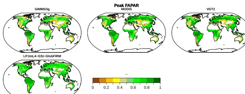
Data on the fraction of absorbed photosynthetically active radiation (FAPAR) are derived from three different satellite datasets to account for differences between datasets for model evaluation (see Table 4, Forkel et al., 2015): the MODIS (USGS, 2001) FAPAR (Knyazikhin et al., 1999), the Geoland2 BioPar (GEOV1) FAPAR dataset (Baret et al., 2013) (hereafter called VGT2 FAPAR), and the GIMMS3g FAPAR dataset (Zhu et al., 2013). The MODIS FAPAR dataset is taken from the MOD15A2 product with a temporal resolution of 8 days at a spatial resolution of 1 km, covering the period 2001 to 2011. VGT2 is based on SPOT VGT with a temporal resolution of 10 days and 0.05◦spatial resolution
(Baret et al., 2013), covering the period 2003 to 2011. The GIMMS3g dataset has a 15-day temporal resolution and 1/12◦ spatial resolution and covers the period from 1982
to 2011. Data on FAPAR are also subject to uncertainties from the processing of the remotely sensed data and are not available continuously for all areas. We compare the spatial patterns of the peak FAPAR, the temporal dynamics of FAPAR in each grid cell, and seasonal variations in FAPAR averaged for Köppen–Geiger climate zones for the three different FAPAR datasets. The aggregated FAPAR represents the average monthly time series for all grid cells that belong to a certain Köppen–Geiger climate zone (see also Forkel et al., 2015). For the Köppen–Geiger climate zones, FAPAR time series are averaged over all grid cells that belong to the same Köppen–Geiger climate zone (see also Forkel et al.,
2015). For the evaluation of the reflectance of the Earth’s surface we used the MODIS C5 albedo time series dataset (https://lpdaac.usgs.gov/dataset_discovery/modis/modis_ products_table/mcd43c3) from 2000–2010 (Lucht et al., 2000; Schaaf et al., 2002), which we also aggregated to Köppen–Geiger climate zones for the evaluation here.
2.2.8 Agricultural productivity
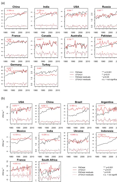
Detailed data on crop growth and productivity are available for individual sentinel sites (Rosenzweig et al., 2014). For global-scale or regional simulations, reference data are avail-able only for crop yields and in (sub-)national aggregations (e.g. FAO-AQUASTAT, 2014) or as processed and interpo-lated gridded products (Iizumi et al., 2014). In all yield data statistics outside of well-controlled field experiments, yield levels and inter-annual variability are not only affected by variability in weather, but also by variance in management conditions, such as sowing dates, variety choices, cropping areas, fertilizer inputs, and pest control (Schauberger et al., 2016). Consequently, it is difficult to evaluate model perfor-mance from a comparison of simulated yields with static as-sumptions on most management aspects with yield statistics in which the contribution of weather variability to yield vari-ability is unknown. Müller et al. (2017) propose a combi-nation of global gridded crop model simulations and differ-ent observation-based yield datasets to establish a benchmark for global crop model evaluation. Generally, global gridded crop models perform well in most regions for which sta-tistical models can detect a significant influence of weather on crop yield variability (Ray et al., 2015). We here evalu-ate LPJmL4 by comparing the simulevalu-ated and observed yield variability of the 10 top-producing countries of the respec-tive crop (FAO-AQUASTAT, 2014). We refrain from com-paring to individual sentinel sites, but refer to the evaluation of LPJmL crop simulations at global, national, and grid cell scale in the global gridded crop model evaluation framework (Müller et al., 2017). As in Müller et al. (2017), we aggregate simulated grid-cell-level yield time series to average national yield time series using the MIRCA2000 dataset for spatial aggregation (Porwollik et al., 2016) and removing trends in observations and simulations with a moving-window aver-age (see Müller et al., 2017, for details). The productivity of biomass plantations is evaluated with data from experimen-tal sites forMiscanthus, switchgrass, poplar, willow, and
2.2.9 Sowing dates
To evaluate the accuracy of the simulated rain-fed sowing dates, we use the global dataset of growing areas and grow-ing periods, MIRCA2000 (Portmann et al., 2008, 2010), at a spatial resolution of 0.5◦ and a temporal resolution of
1 month, as proposed by Waha et al. (2012). Monthly data in MIRCA2000 were converted to daily data by assuming that the growing period starts on the first day of the month fol-lowing Portmann et al. (2010). MIRCA2000 reports several growing periods in a year for some administrative units for the crops wheat, rapeseed, rice, cassava, and maize. For com-parison we select the best corresponding growing period so that a close agreement indicates that simulated sowing dates are reasonable, but not necessarily the most frequently cho-sen by farmers. We do not compare simulated sowing dates for sugar cane (see Fig. S94 in the Supplement) to observed sowing dates, as MIRCA2000 assumes it is grown all year-round as a perennial crop.
2.3 Evaluation metrics
We employ Taylor diagrams (Taylor, 2001) to compare the correlation, differences in standard deviation, and the cen-tred root mean squared error (CRMS) between simulated and observed carbon and water fluxes at FLUXNET sites (ORNL DAAC, 2011) and at gauge stations from ArcticNET and UNH/GRDC. The standard deviations of the reference datasets have been normalized to 1.0 so that multiple sites can be displayed in one figure.
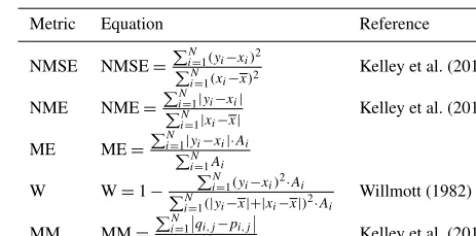
For global gridded reference datasets, such as for carbon stocks, we show spatial patterns in maps and aggregations as latitudinal means and quantify overall differences as a spatial correlation analysis over all grid cells (see Table 4). As sug-gested by Kelley et al. (2013) we use the normalized mean square error (NMSE) to describe differences between model simulation and reference datasets. The NMSE is zero for per-fect agreement, 1.0 if the model is as good as using the data mean as a predictor, and larger 1.0 if the model performs less well than that. The squared error term puts stronger empha-sis on large deviations between simulations and observations and is thus stricter than the normalized mean error (see Ta-ble 1 for equations). Kelley et al. (2013) also suggest using the normalized mean error (NME) as a more robust metric than NMSE. NME is based on absolute residuals (NMSE on squared residuals) and thus is especially better suited for vari-ables that can have very large values and residuals. Addition-ally, we use the Manhattan metric (MM) proposed by Kelley et al. (2013) for evaluation of vegetation cover. Values for MM less than 1 reflect the fact that the model performs bet-ter than the mean value. Additionally, we show the random model, which was generated by bootstrap resampling of the observations as proposed by Kelley et al. (2013, Table 4). The random model was used for the evaluation of vegetation dis-tribution. Table 2 gives an overview of variables evaluated at
Table 1.Evaluation metrics used in this study.
Metric Equation Reference
NMSE NMSE=
PN
i=1(yi−xi)2
PN
i=1(xi−x)2
Kelley et al. (2013)
NME NME=
PN
i=1|yi−xi|
PN
i=1|xi−x|
Kelley et al. (2013)
ME ME=
PN
i=1|yi−xi|·Ai
PN
i=1Ai
W W=1−
PN
i=1(yi−xi)2·Ai
PN
i=1(|yi−x|+|xi−x|)2·Ai
Willmott (1982)
MM MM=
PN
i=1qi,j−pi,j
N Kelley et al. (2013)
Note:yiis the simulated andxithe observed value in grid celli,xthe mean observed
value,Aithe area weight in grid celli, andNthe number of grid cells or sites;qi,jis the
simulated andpi,jis the observed fraction of itemjin grid celli. Normalized mean square error – NMSE, normalized mean error – NME, ME – mean absolute error, W – Willmott coefficient of agreement, MM – Manhattan metric.
the local scale and the measures that were used for the eval-uation of time series for crop yields. We employ a simple time series correlation analysis after removing trends with a moving-window detrending method. For comparison with point measurements, we extract the time series from corre-sponding 0.5◦ grid cells. These simulated time series may
differ in terms of weather and soil conditions from the actual site as the simulations are based on gridded global dataset inputs. The time period is given by the respective measure-ments, which differ for each observation point.
To envisage the degree of agreement between simulated (LPJmL4) and observed (MIRCA2000) sowing dates, we follow Waha et al. (2012) and compute two different met-rics: the Willmott coefficient of agreement (W) (Willmott, 1982) and the mean absolute error (ME), both weighted by the crop-specific cultivated area according to Portmann et al. (2010). For an overview of all metrics used, see Table 1.
3 Results and discussion
In the following we compare the standard version LPJmL4, which refers to the experiment LPJmL4-GSI-GlobFIRM. In the case of the other experiments we refer to the names de-fined in Sect. 2.1.
3.1 Vegetation cover
LPJmL4 reproduces the observed vegetation distribution bet-ter than the random model (Table 3). LPJmL4 can best re-produce the distinction between bare soil and vegetated areas (MM=0.22) and between tree-covered areas and areas
with-out trees (MM=0.31), but with considerably better scores
than the random model (MM=0.56 and 0.54, respectively).
Moreover, LPJmL4 simulation results reach the lowest MM scores for the distinction of evergreen vs. deciduous trees (MM=0.52) and for the distribution and composition of life
forms (trees vs. herbaceous vs. bare soil; MM=0.45); these
Table 2.Overview of variables and measures used for the evaluation of LPJmL4 local scale.
Measure Reference
Standard Reference
Variable CRMSE deviation Correlation to figures Data Citation
CO2 x Figs. 1, 2 Atmospheric transport1 Rödenbeck (2005)
NEE x x x Fig. 3 FLUXNET2 ORNL DAAC (2011)
ET x x x Fig. 7 FLUXNET2 ORNL DAAC (2011)
NPP x Fig. 4d Luyssaert et al. (2007)
GPP x Fig. 4c Luyssaert et al. (2007)
BIOMASS x Fig. 4a, b Luyssaert et al. (2007)
DISCHARGE x x x Figs. 8, ArcticNET3,
S19–S66 UNH/GRDC4 Vörösmarty et al. (1996)
Centred root mean square error (CRMSE).1http://pubman.mpdl.mpg.de/pubman/faces/viewItemOverviewPage.jsp?itemId=escidoc:1691952;
2http://fluxnet.fluxdata.org/data/la-thuile-dataset/;3http://www.r-arcticnet.sr.unh.edu/v4.0/index.html;4http://www.grdc.sr.unh.edu/index.html.
Table 3.Comparison metric scores for LPJmL4 simulations against
observations of fractional vegetation cover data from International Satellite Land-Surface Climatology Project (ISLSCP) II vegetation continuous field (VCF) (Defries and Hansen, 2009).
Vegetation cover Manhattan metric (MM)
LPJmL4 Random model∗
Life forms 0.45 0.88
Tree vs. non-tree 0.31 0.54
Herb vs. non-herb 0.42 0.66
Bare vs. covered ground 0.22 0.56
Evergreen vs. deciduous 0.52 0.87
Broadleaf vs. needle-leaf 0.37 0.94
MM suggested by Kelley et al. (2013),∗values taken from Kelley et al.
(2013, Table 4).
and 0.88, respectively). The largest improvement in LPJmL4 simulations over the random model is found for the pat-terns of broadleaved vs. needle-leaved trees (MM=0.37 for
LPJmL4 vs. 0.94 for the random model; see Table 3).
3.2 Atmospheric CO2concentration and NEE
3.2.1 Comparison of simulated NBP to atmospheric CO2concentration at MLO and BRW
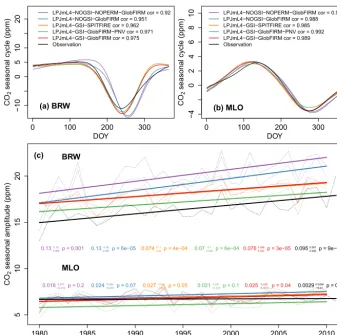
LPJmL4 reproduces the observed long-term and seasonal dynamics of atmospheric CO2 well (Figs. 1 and 2). The
long-term trend of atmospheric CO2 is reproduced well in
all the different model ups (Fig. 1), except for the set-up with natural vegetation only GSI-GlobFIRM-PNV). The experiment with all processes included (LPJmL4-GSI-GlobFIRM) gives the best correlation and trend re-production, which suggests that an integral representation of the LPJmL4 features is required to match observations best. Next to land use dynamics, the inclusion of per-mafrost dynamics has the strongest effects on the
sim-Figure 1.Comparison of the atmospheric CO2 concentrations at
Point Barrow (BRW; panela) and Mauna Loa (MLO; panelb) for
the different LPJmL4 experiments.
ulated trend (LPJmL4-NOGSI-NOPERRM-GlobFIRM vs. LPJmL4-NOGSI-GlobFIRM). The use of the process-based fire model SPITFIRE leads to a small overestimation of the trend in atmospheric CO2 concentrations compared to the
other model set-ups, especially at MLO. Seasonal variations in atmospheric CO2 can be reproduced well by LPJmL4,
phenol-DOY
CO
2
seasonal cycle (ppm)
0 100 200 300
−10
0
5
10
20
LPJmL4−NOGSI−NOPERM−GlobFIRM cor = 0.92 LPJmL4−NOGSI−GlobFIRM cor = 0.951 LPJmL4−GSI−SPITFIRE cor = 0.962 LPJmL4−GSI−GlobFIRM−PNV cor = 0.971 LPJmL4−GSI−GlobFIRM cor = 0.975 Observation
(a) BRW
DOY
CO
2
seasonal cycle (ppm)
0 100 200 300
−4
0
2
4
6
8
10 LPJmL4−NOGSI−NOPERM−GlobFIRM cor = 0.988
LPJmL4−NOGSI−GlobFIRM cor = 0.988 LPJmL4−GSI−SPITFIRE cor = 0.985 LPJmL4−GSI−GlobFIRM−PNV cor = 0.992 LPJmL4−GSI−GlobFIRM cor = 0.989 Observation
(b) MLO
CO
2
seasonal amplitude (ppm)
1980 1985 1990 1995 2000 2005 2010
5
10
15
20
0.13 0.15
0.065 p = 0.001 0.13 0.16
0.097 p = 6e−05 0.074 0.11
0.04 p = 4e−04 0.07 0.1
0.038 p = 6e−040.076
0.095
0.052 p = 3e−05 0.095 0.097 0.046 p = 9e−05
0.018 0.017
−0.013 p = 0.2 0.024 0.025
−0.012 p = 0.07 0.027 0.029
−0.006 p = 0.05 0.021 0.021
−0.012 p = 0.1 0.025
0.025
−0.0077 p = 0.04 0.0029 0.0059 −0.01 p = 0.9
(c)
BRW
MLO (c)
Figure 2.Comparison of the atmospheric CO2concentration at Mauna Loa (MLO) and Point Barrow (BRW) simulated in the different
LPJmL4 experiments.(a, b)Seasonal cycle,(c)trend of the seasonal amplitude, and slopes are given for the different LPJmL4 experiments.
ogy scheme (LPJmL4-NOGSI-GlobFIRM vs. GSI-GlobFIRM; Fig. 2a, b). All model set-ups (except LPJmL4-GSI-SPITFIRE) can reproduce the observed strong signifi-cant increase in the seasonal CO2amplitude at BRW and the
weak (and insignificant) increase at MLO (Fig. 2c). These results are in agreement with a previous evaluation of simu-lated seasonal CO2changes in LPJmL (Forkel et al., 2016).
Further analysis shows that the standard set-up (LPJmL4-GSI-GlobFIRM) can best produce the mean seasonal cycle in MLO, whereas the version that omits land use (LPJmL4-GSI-GlobFIRM-PNV) performs slightly better than this in BRW (Fig. 2). The standard set-up (LPJmL4-GSI-GlobFIRM) can also best reproduce the increase in the sea-sonal amplitude at BRW, whereas it is the only set-up that produces a statistically significant but still very small in-crease in the seasonal amplitude at MLO where observations also do not show a statistically significant increase.
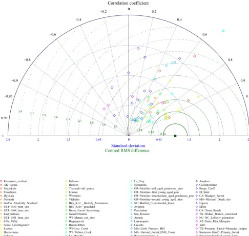
3.2.2 Comparison of simulated NEE to eddy flux measurements
We evaluate the model performance of simulated NEE from LPJmL4 for temporal and spatial variation in NEE data from eddy flux measurements using Taylor diagrams (Taylor, 2001). Stations are sorted from north to south (see Fig. 3) for all NEE measurements available for>3 years. The model is
able to reproduce the mid-latitudes best (represented by yel-low over green to light blue colours), with correlation coeffi-cients mostly between 0.4 and 0.9 and standard deviations of-ten within±30 % of the reference data. The northernmost
re-gions are reproduced well at some flux towers, but often with higher standard deviation than in the flux tower data, which means that the simulated time series are largely in phase but more variable than the observations. In contrast, the evalu-ation is comparatively poor for tropical regions, especially the station at Santarém with strong negative correlations (r <
−0.6) but realistic standard deviations. For this site, however,
00
0.2 −0.2
0.4 −0.4
0.6 −0.6
0.8 −0.8
0.9 −0.9
0.95 −0.95
0.99 −0.99
1
−1 0.52 0.26
0.78 1 1.3 1.6 1.8 2.1 2.3 2.6 2.9 3.1 3.4
00
0.65 0.65
1.3 1.3
2 2
2.6 2.6
Standard deviation
Centred RMS difference Correlation coefficient
Kaamanen_wetland AK−Ivotuk Sodankyla Flakaliden Hyytiala Norunda
Griffin−Aberfeldy−Scotland UCI−1930_burn_site UCI−1964_burn_site East_Saltoun UCI−1981_burn_site Lille_Valby Soroe−LilleBogeskov Loobos Horstermeer Cabauw Brasschaat Mehrstedt
Gebesee Hainich Tharandt−old_spruce Lonzee Wetzstein Vielsalm
Bily_Kriz−_Beskidy_Mountains Bily_Kriz−_grassland Hesse_Forest−Sarrebourg Neustift/Stubai WI−Mature_red_pine Bugacpuszta Renon/Ritten WI−Lost_Creek WI−Willow_Creek La_Mandria
MI−Univ._of_Mich._Biological_station Zerbolo−Parco_Ticino−_Canarazzo
Le_Bray Nonantola
OR−Metolius−old_aged_ponderosa_pine OR−Metolius−first_young_aged_pine OR−Metolius−intermediate_aged_ponderosa_pine OR−Metolius−second_young_aged_pine NH−Bartlett_Experimental_forest Avignon
Puechabon San_Rossore Aurade Lamasquere Lecceto
MA−Little_Prospect_Hill MA−Harvard_Forest_EMS_Tower Roccarespampani_1 Roccarespampani_2 Vall_d'Alinya
Amplero Castelporziano Borgo_Cioffi El_Saler CA−Blodgett_Forest MO−Missouri_Ozark_site Espirra
Mitra CA−Tonzi_Ranch TN−Walker_Branch_watershed NC−NC_Loblolly_plantation AZ−Santa_Rita_Mesquite Yatir
TX−Freeman_Ranch−Mesquite_Juniper Santarem−Km67−Primary_forest Santarem−Km83−Logged_forest
Figure 3.Net ecosystem exchange rate measured at eddy flux towers: ORNL DAAC (2011). Available online at FLUXNET (http://fluxnet.
fluxdata.org/data/la-thuile-dataset/). Sites (colours) are ordered from north to south.
growth observations and model predictions, which is also the case for LPJmL4. We stress that this evaluation is done for a standard LPJmL4 run and standard input (the LPJmL4-GSI-GlobFIRM as described in Schaphoff et al., 2018c); i.e. we did not calibrate the model to site-specific conditions and also drive the model with gridded input data rather than the observed soil and weather data at individual stations. More detail for comparisons with eddy flux tower measurements
Table 4.Overview of variables evaluating LPJmL4 showing measures and references at the global scale.
Measure Reference
Spatial Temporal Visual
Variable NME NMSE correlation correlation comparison Data Citation
GPP – Av 0.20 0.13 0.87 Figs. 5, GPP1 Jung et al. (2011)
S68
Re– Av 0.67 0.55 0.67 Figs. 6, Jägermeyr et al. (2014)
S70
SoilC – Av 0.48 0.75 0.29 Fig. S67 Soil carbon stocks1 Carvalhais et al. (2014)
VegC – Av 0.33 0.36 0.84 Fig. S69a Total biomass1 Carvalhais et al. (2014)
Fig. S69b AGB Liu et al. (2015)
FAPAR – I-aMv 0.17 0.13 0.63 Fig. 10a MODIS FAPAR2 Knyazikhin et al. (1999)
FAPAR – I-aMv 0.18 0.15 0.59 Fig. 10b GIMMS3g FAPAR3 Zhu et al. (2013)
FAPAR – I-aMv 0.21 0.20 0.69 Fig. 10c VGT2 FAPAR4 Baret et al. (2013)
ET 1E-6 0.07 0.84 Fig. S71 Latent heat flux1 Jung et al. (2011)
fBA Fig. S72 GFED4 & CCI Fire (4.1)
Albedo Fig. S72 MODIS C5 Lucht et al. (2000)
Discharge ArcticNET5, Vörösmarty et al. (1996)
Ov 0.42 0.24 R2=0.90 UNH/GRDC6
Mav 0.36 0.19 R2=0.92
I-av 0.24 0.06 R2=0.97
Normalized mean error (NME) and normalized mean square error (NMSE) as suggested by Kelley et al. (2013); Av – annual average; I-aMv – inter-annual monthly variability; overall variability – Ov; monthly average variability – Mav; inter-annual variability – I-av; vegetation carbon – VegC; aboveground biomass – AGB; soil carbon – SoilC; fBA – fractional burnt area.
1https://www.bgc-jena.mpg.de/geodb/BGI/Home;2https://lpdaac.usgs.gov/dataset_discovery/modis/modis_products_table/mod15a2;
3http://cliveg.bu.edu/modismisr/lai3g-fpar3g.html;4http://cordis.europa.eu/result/rcn/140496_en.html;5http://www.r-arcticnet.sr.unh.edu/v4.0/index.html;
6http://www.grdc.sr.unh.edu/index.html.
3.3 Vegetation and soil carbon stocks and vegetation productivity
3.3.1 Soil carbon and vegetation carbon stocks
The spatial correlation between simulated and observation-based estimates of SOC by Carvalhais et al. (2014) is weak (r=0.29; Table 4) with disagreements in the subtropics
where LPJmL4 simulations substantially underestimate soil carbon stocks, whereas LPJmL4 reports much higher soil carbon in the high northern latitudes (>50◦N) and lower
values for the tropical and temperate zone compared to Car-valhais et al. (2014) (see Fig. S67). Other estimates by Tarnocai et al. (2009) show much higher carbon content for the permafrost-affected areas than the dataset of Carvalhais et al. (2014). We thus assume that the disagreement between simulations and the Carvalhais et al. (2014) data may also result from an underestimation of carbon stocks in the Car-valhais et al. (2014) data. However, the estimation of global soil carbon is less in LPJmL4 (1869 Pg C) than estimated by Carvalhais et al. (2014) (2352±400 Pg C).
The comparison of simulated and observation-based as-sessments of vegetation carbon show a good spatial correla-tion (r=0.84; Table 4). Globally, Carvalhais et al. (2014)
es-timate slightly lower biomass (445±8 Pg C) as simulated by
LPJmL4 (507 Pg C). The spatial patterns of vegetation
car-bon stocks are shown in Fig. S69a for simulations and the data product of Carvalhais et al. (2014). While the broad ge-ographical patterns are in overall agreement with the evalua-tion data, the absolute values differ in some regions. Specif-ically, LPJmL4 simulates much higher biomass (see the lati-tudinal pattern in Fig. S69) for the tropics and lower biomass between 20 and 40◦ in the Northern and Southern
● ● ● ● ● ● ● ● ● ● ● ● ● ● ● ● ● ● ● ● ● ● ● ● ● ● ● ● ● ● ● ● ● ● ● ● ● ● ● ● ● ● ● ● ● ● ● ● ● ● ● ● ● ● ● ● ● ● ● ● ● ● ● ● ● ● ● ● ● ● ● ● ● ● ● ●
0 5 10 15 20 25 30 35
0 5 10 15 20 25 30 35 Vegetation carbon
Observed[kgCm−2]
LPJmL4
[kgC
m
−
2]
R2= 0.13 s = 0.35 p = 0.00136 RMSE = 7.02 NMSE = 1.28 NME = 1.14
(a) ● ● ● ● ● ● ● ● ● ● ● ● ● ● ● ● ● ● ● ● ● ● ● ● ● ● ● ● ● ● ● ● ● ● ● ● ● ● ● ● ● ● ● ● ● ● ● ● ● ● ● ● ● ● ● ● ● ● ● ● ● ● ● ● ● ● ● ● ● ● ● ● ● ● ● ● ● ● ● ● ● ● ● ● ● ● ● ● ● ● ● ● ● ● ● ● ● ● ● ● ● ● ● ● ● ● ●
0 10 20 30
0 10 20 30
Aboveground biomass
Observed[kgCm−2]
LPJmL4
[kgC
m
−
2]
R2= 0.08 s = 0.32 p = 0.00296 RMSE = 6.51 NMSE = 1.66 NME = 1.21
(b) ● ●● ● ● ●● ● ● ● ● ● ● ● ● ● ● ● ● ● ● ● ● ● ● ● ● ● ● ● ● ● ● ● ● ● ● ● ● ● ● ● ● ● ● ● ● ● ● ● ● ● ●● ● ● ● ● ● ● ●● ● ● ● ● ● ● ● ● ● ● ● ● ● ● ● ●● ● ● ● ● ● ● ● ● ● ● ● ● ● ● ● ●
0 1 2 3 4
0 1 2 3 4 GPP
Observed[kgCm−2a−1)]
LPJmL4 [kgC m − 2a − 1)]
R2= 0.31 s = 0.33 p = 0 RMSE = 0.75 NMSE = 1 NME = 0.89
(c) ● ● ● ● ●● ● ● ● ● ● ● ● ● ●● ● ● ● ● ● ● ● ● ● ● ● ● ● ●● ● ● ● ● ● ● ● ● ● ● ● ●● ● ● ● ● ●●● ● ● ● ● ● ● ●● ● ● ● ● ● ● ● ● ● ● ● ●●●● ● ● ● ● ● ● ● ● ● ● ● ● ● ● ● ● ●
0.0 0.5 1.0 1.5
0.0 0.5 1.0 1.5
NPP
Observed[kgCm−2a−1)]
LPJmL4 [kgC m − 2a − 1)]
R2= 0.23 s = 0.3 p = 0 RMSE = 0.31 NMSE = 1.15 NME = 1
(d)
Figure 4.Evaluation of vegetation carbon(a), aboveground biomass(b), GPP(c), and NPP(d). Observed data are provided by Luyssaert
et al. (2007). Bars give the minimum and maximum of the estimation within one 0.5◦cell simulated by LPJmL4.
show a high overestimation of biomass in the high latitudes. Similarly, the inclusion of the GSI phenology substantially reduces the biomass overestimation in comparison to Car-valhais et al. (2014) and Liu et al. (2015), which is consistent with the finding of Forkel et al. (2014). The consideration of human land use in the simulations improves carbon stock simulations in the temperate zones (Fig. S69). This clearly demonstrates the importance of permafrost, human land use, and the GSI phenology for the simulation of the terrestrial carbon cycle, even though the remaining discrepancies war-rant further model improvement.
Figure 4a and b compare site data estimation with the rep-resentative LPJmL4 grid cell estimation with an uncertainty range which comes from the different measurements within one 0.5◦grid cell. Both vegetation and aboveground carbon
are slightly overestimated in some cases but also strongly un-derestimated in others. As LPJmL4 calculates a representa-tive mean value of a 0.5◦ grid cell for all benchmarks, the
simulated values should match the mean values. However, it can be assumed that measurements are not evenly distributed through the age classes within one grid cell or forest, and it remains unclear how representative the measurements are for a 0.5◦grid cell area.
3.3.2 Gross and net primary production (GPP and NPP)
The global estimation of 123.7 Pg C a−1GPP from LPJmL4
(see Fig. 5) matches the estimates from Beer et al. (2010) and Jung et al. (2011) of 123±8 and 119±6 Pg C a−1,
re-spectively, for the years 1982–2005, whereas the highest di-vergence can be observed in the tropics where LPJmL4 timates much lower values despite the higher biomass es-timations (see Sect. 3.3). LPJmL4 simulated higher GPP for the temperate and boreal zones than reported by Jung et al. (2011). The different model experiments show simi-lar patterns except for LPJmL4-GSI-GlobFIRM-PNV, which shows lower GPP in the Mediterranean (see Fig. 5). Carval-hais et al. (2014) estimate global NPP at 54±10 Pg C a−1
and LPJmL4 at 57 Pg C a−1for the mean of the years 1982–
2011.
The site data comparison to Luyssaert et al. (2007) shows a good agreement between site measurements and simulated GPP (see Fig. 4c) and NPP (see Fig. 4d). The overestima-tion of simulated biomass and the good agreement of NPP and GPP leads to the conclusion that LPJmL4 underesti-mates mortality. This warrants further investigation of why LPJmL4 seems to overestimate global GPP but shows good agreement with site data. The comparison of LPJmL4 against MTE data (Jung et al., 2011) on the local scale for the same points as given by Luyssaert et al. (2007) shows a good agreement, especially if outliers are excluded (Fig. S68b, c). Figure S68a compares plot data against the global data.
3.3.3 Ecosystem respiration (Re)
Comparison of satellite-derived ecosystem respiration with that simulated by LPJmL4 reveals similar spatial patterns (Figs. 6 and S70). However, LPJmL4 shows higher temper-ature sensitivities (Fig. 6a) and consistently simulates higher
Revalues in high-latitude and subtropical regions (Fig. S70).
Since satellite-derived ecosystem respiration is calibrated for FLUXNET data and hence exhibits marginal cross-latitude bias, the discrepancies to LPJmL4 are likely associated either with LPJmL4 parameterization or with systematic errors in the FLUXNET processing technique. Additional details and figures are presented in Jägermeyr et al. (2014).
3.4 Water fluxes
3.4.1 Evapotranspiration
MTE
LPJmL4−GSI−GlobFIRM
Gross primary production
0 400 800 1200 1800 2400 3000
gC m−2 a−1
−40 −20 0 20 40 60 80
0 500 1500 2500 3500 MTE LPJmL4−GSI−GlobFIRM LPJmL4−NOGSI−GlobFIRM LPJmL4−GSI−GlobFIRM−PNV LPJmL4−NOGSI−NOPERM−GlobFIRM LPJmL4−GSI−SPITFIRE (a) (b)
Figure 5.The maps(a)show the spatial pattern of gross primary production (GPP; g C m−2a−1) distribution from the standard LPJmL4
simulation against the MTE data (Jung et al., 2011). The graph in(b)shows the latitudinal pattern of GPP distribution simulated by the
different versions of LPJmL4 against data from Jung et al. (2011).
● ● ● ● ● ● ● ● ● ● ● ● ● ● ●● ● ● ● ● ● ● ● ● ● ● ● ● ● ● ● ● ● ● ● ● ● ● ● ● ● ● ● ● ● ● ● ●● ● ●● ● ● ●● ● ● ● ● ● ● ●●● ● ●● ● ● ●●●● ●● ● ● ● ● ●● ● ● ● ● ●● ● ● ● ● ● ● ● ● ●●●● ● ●● ● ●● ● ● ● ● ●●●●● ● ● ● ● ● ● ● ● ● ● ● ● ● ● ● ● ● ● ● ● ● ● ●● ●● ● ● ● ● ● ● ● ●●● ● ●●●● ● ● ●● ●●● ● ● ● ● ● ● ● ● ● ●● ● ● ● ● ● ● ● ● ● ● ● ● ● ● ● ● ● ● ●● ● ● ● ●●● ● ●● ● ● ● ● ● ● ● ●●● ●● ● ● ● ● ● ● ●●● ● ● ● ● ● ●●● ● ● ● ● ● ● ● ● ● ●●●● ● ●● ● ●●●●● ● ●● ● ● ● ● ● ●●●●●● ● ●● ● ●●● ● ● ● ● ● ● ● ● ● ● ● ● ● ● ● ●●● ● ● ●● ● ● ●● ●● ● ● ● ● ● ● ● ● ● ● ●●● ● ● ● ● ●●● ● ● ●● ● ● ● ● ● ● ● ● ● ● ● ● ● ● ● ●● ● ●● ●● ● ● ● ● ● ●●● ● ● ● ● ●● ● ●● ● ● ●● ● ● ● ● ● ●●● ●● ● ●● ● ● ● ●● ● ● ● ● ● ● ● ● ● ● ● ● ● ● ● ● ● ●● ● ● ● ● ● ● ● ●●● ●● ● ● ● ● ● ● ● ● ● ● ● ● ● ● ●● ● ● ● ● ● ● ● ● ●●● ● ● ● ● ● ● ● ● ● ● ● ● ● ●●● ● ● ● ● ● ● ● ● ●● ● ● ● ● ● ● ● ●● ●● ● ● ● ●●● ● ● ● ● ● ● ● ● ● ● ● ● ● ● ●●● ● ●● ●● ● ● ● ● ● ● ● ● ●● ● ● ● ● ●● ●● ● ● ● ● ● ● ● ● ● ●● ● ● ●● ●● ● ● ● ● ● ● ● ● ●● ● ● ● ● ● ● ● ● ● ● ●● ● ● ● ● ● ● ● ● ● ● ● ● ● ● ● ● ● ● ● ● ● ● ● ● ● ● ●● ●● ● ● ● ● ● ● ● ● ● ● ● ● ● ● ● ●● ● ● ● ● ●● ● ● ● ● ● ● ● ● ●● ● ● ●●● ● ● ● ● ● ● ● ● ● ● ● ● ● ● ● ● ● ● ● ● ● ● ● ● ● ● ● ● ● ● ● ● ● ● ● ● ● ● ● ● ● ●●● ● ● ● ● ● ● ● ●● ●● ● ●● ● ● ● ● ● ● ● ● ● ● ● ● ● ● ● ● ● ● ● ●● ● ● ● ● ● ● ● ● ● ● ● ● ● ●● ● ● ● ● ● ●● ● ●● ●● ● ● ● ● ●● ● ●● ● ● ● ●● ● ● ● ● ● ●●● ● ●● ● ●● ● ● ● ● ● ● ● ● ● ● ● ● ● ● ● ● ● ● ● ●●● ● ● ● ● ●● ● ● ● ● ● ● ● ● ● ● ● ●●● ● ● ● ● ● ●● ● ● ● ● ● ● ● ● ● ● ● ● ● ● ● ● ● ● ● ● ● ●● ● ● ● ● ●● ● ● ● ● ● ● ● ● ● ● ● ● ● ● ● ● ● ● ● ● ● ● ● ● ● ● ● ● ● ●● ● ● ● ● ● ● ● ● ● ● ● ● ● ● ●● ●●● ● ● ● ● ● ● ● ● ● ● ●● ●● ● ● ● ● ● ● ● ● ● ● ● ● ● ● ● ● ● ● ●●●●●●●● ● ●● ●●● ● ● ● ● ● ● ● ● ● ● ● ● ● ●● ● ● ● ● ● ● ● ● ●● ● ● ● ● ● ●● ● ● ● ● ● ● ● ● ● ● ● ● ● ● ● ● ● ●● ● ● ● ● ● ● ● ● ● ● ● ● ● ● ● ● ● ● ● ● ● ● ●● ● ● ● ● ● ● ● ● ● ● ●● ● ● ● ● ● ● ●● ● ● ● ●● ● ● ● ● ● ● ● ● ● ● ● ● ●● ● ● ● ● ● ●● ● ● ● ● ● ● ● ● ● ● ● ● ●● ● ● ● ● ● ● ● ● ● ● ● ● ● ● ● ● ● ● ● ● ● ● ● ● ● ● ● ● ● ● ● ● ● ● ● ● ● ● ● ● ● ●● ● ● ● ● ●●● ● ● ● ● ●● ● ● ● ●● ● ● ● ● ● ● ● ● ● ● ● ● ●● ● ● ● ● ● ●●● ● ●●●● ● ● ● ●● ●● ● ● ● ● ● ● ● ● ● ● ●● ● ● ● ● ● ● ● ● ● ● ● ● ● ● ● ● ● ● ● ● ● ● ● ● ● ● ● ● ● ● ● ● ● ● ● ● ● ●●● ● ● ● ● ● ● ● ● ● ●● ● ● ● ● ● ● ● ●● ● ● ●● ● ● ● ● ● ● ● ● ● ● ● ●● ● ● ● ● ● ● ● ●● ● ● ● ● ● ●● ●● ● ● ●●●●● ● ● ● ● ● ● ● ● ● ● ● ● ● ● ● ● ● ●● ● ● ● ● ● ● ● ● ● ●●● ● ●● ● ● ● ●● ● ●● ● ● ● ● ● ● ● ● ●● ● ● ● ● ● ● ● ● ● ● ● ●● ● ● ● ● ● ● ● ● ● ● ● ● ● ● ● ● ● ●●●● ● ● ● ●●●● ● ● ● ● ● ● ● ● ● ● ● ● ● ● ● ● ● ● ● ● ● ● ● ● ● ●● ●● ● ● ●● ● ● ● ●● ● ● ● ● ● ● ● ● ● ● ● ● ● ● ● ● ● ● ● ● ● ● ● ● ● ● ● ● ● ● ● ● ● ● ●● ● ● ● ● ● ● ● ●● ● ● ● ● ● ● ● ● ● ● ● ● ● ● ● ● ● ● ● ● ● ● ● ● ● ● ● ● ● ● ● ● ●● ● ● ● ●●● ● ● ● ● ● ● ● ● ● ● ● ● ●● ● ● ● ●● ●● ● ● ● ● ● ● ● ● ● ● ● ● ● ● ● ● ● ● ● ● ● ● ● ● ●●● ● ● ● ● ●● ●● ● ● ● ●●● ● ●● ● ● ● ● ● ● ● ● ● ● ● ● ● ● ● ●● ● ● ● ● ● ● ● ● ● ● ● ● ● ● ● ● ●● ● ● ● ● ● ● ● ● ● ● ● ● ● ● ● ● ● ● ● ● ● ● ● ● ● ● ● ● ● ● ● ● ● ● ● ● ● ● ● ● ● ● ● ● ●● ● ● ● ● ● ● ● ● ● ● ● ● ● ● ● ● ● ● ● ● ● ● ● ● ● ● ● ● ● ● ● ● ● ● ● ● ● ●● ● ● ●
0 500 1000 1500 2000 2500
0 500 1000 1500 2000 2500
LPJmL4 annual Re (g C m−2 a−1)
R E C O a nn ua l R e ( g C m
−2 a −1)
1/1 line
(a)
R2= 0.69
NMSE = 0.7 NME = 0.86
●FOR GRA/CRO Flux tower Temperature limited ● ● ● ● ● ● ● ● ● ●●● ● ● ●● ●●●● ●●● ● ● ● ● ● ● ● ●● ● ● ● ● ● ●● ●● ●●● ● ● ● ● ● ● ● ● ● ● ● ● ● ● ● ● ● ● ● ●● ● ● ● ● ●●● ● ● ● ● ● ● ● ●● ● ● ● ● ● ●●● ● ● ● ● ● ● ● ● ● ●● ● ● ● ● ● ●●● ● ●● ● ● ●● ●●●●●●●● ● ● ● ●● ● ● ●●●● ● ● ● ● ● ● ● ● ● ● ● ● ● ● ● ● ● ● ●●● ●● ● ● ●● ● ● ●● ● ● ● ● ● ● ● ●● ● ● ● ●●● ● ● ● ●●● ● ●●● ●●●● ●● ● ● ● ● ● ● ● ●● ● ● ● ● ● ●● ● ● ● ● ●●●● ● ● ● ● ● ● ● ● ● ● ● ● ● ● ● ●●● ● ● ● ● ● ●● ● ● ● ● ● ● ● ● ● ● ●● ● ● ● ● ● ● ●● ● ● ● ● ● ● ● ● ● ● ● ● ● ● ● ● ● ● ● ● ●● ● ● ● ● ● ● ● ● ● ● ● ● ● ● ●● ● ● ● ● ● ● ● ● ● ● ●●● ●● ●● ● ● ● ● ● ● ● ● ● ● ● ● ● ● ● ● ●● ● ● ● ● ● ● ● ● ● ● ● ●● ● ● ● ●● ● ● ● ● ● ● ●● ●●●● ●● ● ● ● ● ● ● ● ● ●●●● ● ● ● ● ● ● ● ● ● ● ●● ● ●● ● ● ● ● ● ● ● ● ● ● ● ● ● ● ● ●● ● ● ● ● ● ●●● ●● ● ● ● ● ● ● ● ● ● ●●● ● ● ●● ● ● ● ● ● ● ● ● ● ● ● ● ●● ● ● ● ● ● ● ● ● ● ● ● ● ● ● ● ● ● ● ● ● ● ● ● ● ● ● ● ●● ● ● ● ● ● ● ● ● ● ● ● ● ● ● ● ● ● ● ● ● ● ● ● ● ● ● ● ●● ● ●● ● ● ● ● ● ● ● ● ● ● ● ● ● ● ● ● ● ● ● ● ● ●● ● ●● ● ● ● ● ● ● ● ● ● ● ● ●● ● ● ● ● ● ● ● ● ● ● ● ● ● ● ● ● ● ● ● ● ● ● ● ● ● ● ● ● ● ● ● ● ● ● ● ● ● ● ● ●● ●● ● ● ● ● ● ● ● ● ●● ● ● ● ● ● ● ● ● ● ● ● ● ● ● ● ● ● ● ● ● ● ● ● ● ● ● ● ● ● ● ● ● ●● ● ● ● ● ● ● ● ● ● ● ●● ● ● ● ●● ● ●● ● ● ● ● ● ● ● ● ● ● ● ● ● ● ● ● ● ●● ● ● ● ● ● ● ● ● ● ● ● ● ● ● ● ● ● ● ● ● ● ● ● ● ● ● ● ● ● ● ● ●● ● ● ● ●● ● ● ● ● ● ● ● ● ● ● ● ● ● ● ● ● ● ● ● ● ● ● ● ● ● ● ● ● ● ● ●●● ● ● ● ● ● ● ● ● ● ● ● ● ● ● ● ● ● ● ● ● ● ● ● ● ● ● ● ● ● ● ● ● ● ●● ● ● ● ● ●● ● ● ● ● ● ● ● ● ● ● ● ● ● ● ● ● ● ● ● ● ● ● ● ● ● ● ● ● ● ● ● ● ● ● ● ● ●●● ● ● ● ● ● ● ●● ● ● ● ●● ● ● ● ● ● ● ● ● ● ● ● ●● ● ● ● ● ● ●● ● ● ● ● ● ● ● ● ● ● ● ● ● ● ●● ● ● ● ● ● ● ● ● ● ● ● ● ● ● ● ● ● ● ● ● ● ● ● ● ● ● ● ● ● ● ● ● ● ● ● ● ● ● ● ●● ● ●● ●● ● ● ● ● ● ● ● ● ●● ● ●● ● ● ● ● ● ●● ●● ● ● ● ● ●● ● ● ● ● ● ● ● ● ● ● ● ● ● ● ● ● ● ● ● ● ● ● ● ● ● ● ● ● ● ● ● ● ● ● ● ● ● ● ● ● ● ● ● ● ● ● ● ● ● ● ● ● ● ● ● ● ● ● ● ● ●● ● ● ● ● ● ● ● ● ● ● ● ● ● ● ● ● ● ● ● ● ● ● ● ● ● ● ● ● ● ● ● ● ● ● ● ● ● ●● ●●● ● ● ● ● ● ● ● ● ● ● ● ● ● ● ● ● ●● ● ● ● ●●●● ● ● ● ● ● ● ● ● ● ● ● ● ● ● ● ● ● ●● ● ● ● ● ● ● ● ● ●● ● ● ● ●● ● ● ● ● ● ● ● ●● ● ● ● ● ● ● ● ● ●● ● ● ● ● ● ●● ● ● ●●●● ● ● ● ● ● ● ● ● ● ● ● ● ● ● ● ● ● ● ● ● ● ● ● ● ● ● ● ● ● ● ● ● ● ● ● ● ● ● ● ● ● ● ● ● ● ● ● ● ● ● ● ● ● ●● ● ● ● ● ● ● ● ● ● ● ● ● ● ● ●● ● ● ● ● ● ● ● ● ● ● ● ● ● ● ● ● ● ● ● ● ● ● ● ● ● ● ● ● ● ● ● ● ● ● ● ● ●● ● ● ● ● ● ● ● ● ● ● ● ● ● ● ● ●● ● ● ● ● ● ● ● ● ● ● ● ● ● ● ● ● ● ● ● ● ● ● ● ● ● ● ● ● ● ● ● ● ● ● ● ● ● ● ● ● ● ● ● ● ● ●●● ● ● ● ● ● ● ●● ● ● ● ● ● ● ● ● ● ● ● ● ● ● ● ● ● ● ● ● ● ● ● ● ●● ● ● ● ● ● ● ● ● ● ●● ● ● ● ● ● ● ● ● ● ● ● ● ● ● ● ● ● ●● ● ● ● ● ● ● ● ● ● ● ● ● ● ● ● ● ● ● ● ● ● ● ● ● ● ● ● ● ● ● ● ● ● ● ● ● ● ● ● ● ● ● ● ● ● ● ● ●● ● ● ● ● ● ● ● ● ● ● ● ● ● ● ● ● ● ● ● ● ● ● ● ●● ● ● ● ● ●● ● ● ● ● ● ● ● ● ● ● ● ● ● ● ● ● ● ● ● ● ● ●● ● ● ● ● ● ● ● ● ● ● ● ● ● ● ● ● ● ● ● ● ● ● ● ● ●● ● ● ● ● ● ● ● ● ● ● ● ● ● ● ●● ● ● ● ● ● ● ● ● ● ● ● ● ● ● ● ● ●● ● ● ● ● ● ● ● ● ● ● ● ● ● ● ● ● ● ● ● ● ● ● ● ● ●● ● ● ● ● ● ● ● ● ● ● ● ● ● ● ● ● ● ● ● ● ● ● ● ● ● ● ● ● ● ● ● ● ● ● ● ● ● ●● ● ● ● ● ● ● ● ● ● ● ● ● ● ● ● ● ● ●● ● ● ● ● ● ● ● ● ● ● ● ● ● ● ● ● ●● ● ● ●● ● ● ● ● ● ● ● ● ● ● ● ● ● ● ● ● ● ● ● ● ● ● ● ●● ● ● ● ●● ● ●●● ● ● ● ● ● ● ●●● ● ●● ● ● ● ● ●● ● ● ● ● ● ● ● ● ● ● ● ● ● ● ●● ● ● ● ●● ● ● ● ● ● ● ● ● ● ● ● ● ● ● ● ● ● ●● ● ● ● ● ● ● ● ● ● ● ● ● ● ● ● ● ●● ● ● ● ● ● ● ● ● ● ● ● ● ● ● ● ● ● ● ● ● ● ● ● ● ● ● ● ● ● ●● ● ● ● ● ● ● ● ● ● ● ● ● ● ● ● ● ● ● ●● ● ● ● ● ● ● ● ● ●●● ● ● ● ● ● ● ● ● ● ● ● ● ● ● ● ● ● ● ● ● ● ● ● ●● ● ● ● ● ● ● ● ● ● ● ● ● ● ● ● ● ● ● ● ● ● ● ●
0 500 1000 1500 2000 2500
LPJmL4 annual Re (g C m−2 a−1)
1/1 line
(b)
R2= 0.41
NMSE = 0.99 NME = 0.95
Temperate humid ● ● ● ● ● ● ● ● ● ● ● ● ● ● ● ● ● ● ● ● ● ● ● ● ● ● ● ● ●
0 500 1000 1500 2000 2500
LPJmL4 annual Re (g C m−2 a−1)
1/1 line
(c)
R2= 0.4
NMSE = 2.54 NME = 1.74
0 500 1000 1500 2000 2500 Water limited
Figure 6.Ecosystem respiration (Re) evaluation of standard LPJmL4 simulations with satellite-derived estimations from Jägermeyr et al.
(2014). AnnualResums for all pixels from the displayed extent in Fig. S70 are compared and separated by climate type(a)–(c). Dashed lines
indicate a polynomial bias curve. Chart symbols are separated for forest (FOR) and grassland–cropland (GRA–CRO) land cover classes.
not with the general overestimation of vegetation biomass (Fig. S69). The different experiments show nearly no ef-fects on the simulated evapotranspiration. At site level, the evapotranspiration fluxes show a good agreement with eddy flux tower measurements (Fig. 7). LPJmL4 shows good per-formance in most regions, with correlation coefficients of-ten larger than 0.6. The northern and temperate stations (red
00
0.2 −0.2
0.4 −0.4
0.6 −0.6
0.8 −0.8
0.9 −0.9
0.95 −0.95
0.99 −0.99
1
−1 0.48 0.24
0.72 0.96 1.2 1.4 1.7 1.9 2.2 2.4 2.6 2.9 3.1 3.4
00
0.6 0.6
1.2 1.2
1.8 1.8
2.4 2.4
Standard deviation
Centred RMS difference Correlation coefficient
AK−Atqasuk Kaamanen_wetland AK−Ivotuk Sodankyla Flakaliden Hyytiala Skyttorp Norunda UCI−1998_burn_site Griffin−Aberfeldy−Scotland UCI−1989_burn_site UCI−1964_burn_site UCI−1930_burn_site East_Saltoun UCI−1981_burn_site Lille_Valby Soroe−_LilleBogeskov Loobos
Horstermeer Cabauw Brasschaat Mehrstedt Hampshire
Gebesee Hainich Tharandt−old_spruce Lonzee Wetzstein Vielsalm
Bily_Kriz−_Beskidy_Mountains Bily_Kriz−_grassland Hesse_Forest−Sarrebourg MT−Fort_Peck Laegeren Oensingen1_grass Oensingen2_crop Neustift/Stubai WI−Mature_red_pine Bugacpuszta Renon/Ritten WI−Lost_Creek WI−Willow_Creek La_Mandria
MI−Univ._of_Mich._Biological_station Zerbolo−Parco_Ticino−_Canarazzo Le_Bray
Nonantola
OR−Metolius−intermediate_aged_ponderosa_pine OR−Metolius−first_young_aged_pine OR−Metolius−second_young_aged_pine NH−Bartlett_Experimental_forest Avignon
Puechabon San_Rossore Aurade Lamasquere Lecceto
MA−Harvard_Forest_EMS_Tower Island_of_Pianosa
MA−Little_Prospect_Hill Roccarespampani_1 Roccarespampani_2 Vall_d'Alinya Amplero Castelporziano
NE−Mead−rainfed_maize−soybean_rotation_site NE−Mead−irrigated_continuous_maize_site NE−Mead−irrigated_maize−soybean_rotation_site Borgo_Cioffi
CO−Niwot_Ridge_forest IL−Bondville NJ−Fort_Dix El_Saler CA−Blodgett_forest MO−Missouri_Ozark_site Espirra
Mitra_IV_Tojal CA−Tonzi_Ranch
OK−ARM_Southern_Great_Plains_site TN−Walker_Branch_watershed NC−NC_Clearcut NC−NC_Loblolly_plantation CA−Sky_Oaks−old_stand AZ−Santa_Rita_Mesquite Yatir
TX−Freeman_Ranch−Mesquite_Juniper FL−Slashpine−Mize−clearcut−3yr FL−Slashpine−Donaldson FL−Slashpine−Austin_Cary Santarem−Km67−Primary_forest Santarem−Km83−Logged_forest
Figure 7.Evaporation rate measured at eddy flux towers: ORNL DAAC (2011). Available online at FLUXNET (http://fluxnet.fluxdata.org/
data/la-thuile-dataset/). Site locations are ordered from north to south.
3.4.2 River discharge stations evaluation
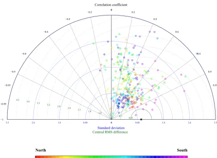
Discharge simulated by earlier LPJmL versions was previ-ously evaluated in several studies, also in comparison with other global hydrological and land surface models (Hadde-land et al., 2011). River discharge was evaluated for major catchments globally, also accounting for the effects of differ-ent precipitation datasets (Biemans et al., 2009) and region-ally for the Amazon basin (Langerwisch et al., 2013) and the Ganges (Siderius et al., 2013). Figure 8 shows the
com-parison of simulated LPJmL4 and observed river discharge values for all gauges with a basin area≥10 000 km2. Here,
00
0.2 −0.2
0.4 −0.4
0.6 −0.6
0.8 −0.8
0.9 −0.9
0.95 −0.95
0.99 −0.99
1
−1 0.35
0.7 1 1.4 1.8 2.1 2.4 2.8 3.2 3.5 3.8 4.2
00
0.88 0.88
1.8 1.8
2.6 2.6
3.5 3.5
Standard deviation
Centred RMS difference Correlation coefficient
North South
Figure 8.Comparison of simulated discharge with 287 gauges provided by ArcticNET (http://www.r-arcticnet.sr.unh.edu/v4.0/index.html)
and UNH/GRDC (http://www.grdc.sr.unh.edu/index.html). Stations with basin area≥10 000 km2are taken into account. Gauges are ordered
from north to south (see legend colour).
(Schaphoff et al., 2013), which is mainly a result of the newly implemented GSI phenology scheme (Forkel et al., 2014). The discharge spring peaks in permafrost areas are especially affected by this improvement. At many gauges, LPJmL4 can reproduce the variability for the whole time series and spe-cially the seasonality, with a highR2and NME and NMSE,
which implies a better performance than the mean model. The dynamics at gauges in the temperate zone (Figs. S49– S50, S61) are not well reproduced in the simulations, and the NME and NMSE also show high values in contrast to gauges in the subtropics and tropics (Figs. S64–S66), which typically show highR2and low NME and NMSE.
The evaluation at the global aggregation (computed for all stations and then averaged) shows very high agreement be-tween observed and modelled discharge (see Table 4). Both the explained variance (R2) and the NME–NMSE contribute
to the good performance of the simulated discharge. The con-stant flow velocity in all rivers, as assumed in LPJmL4 sim-ulations, could be varied by river for further model improve-ment, especially for the timing in flat areas where wetland dynamics may play an important role.
3.4.3 Irrigation withdrawal and consumption
Global estimates of irrigation water withdrawal (Wd:
2545 km3a−1) and consumption (W
c: 1292 km3a−1) agree
well with previous studies. ReportedWdvalues for the period
1998–2012 are 2722 km3a−1(FAO-AQUASTAT, 2014), and
modelling results range from 2217 to 3185 km3a−1 (Döll
et al., 2014, 2012; Wada and Bierkens, 2014; Alexan-dratos and Bruinsma, 2012; Wada et al., 2011; Siebert and Döll, 2010). Wc estimations range between 927 and
1530 km3a−1 (Chaturvedi et al., 2015; Döll et al., 2014;
Hoff et al., 2010). Döll et al. (2012) find that 1179 km3a−1
(1098 km3a−1 in Wada and Bierkens, 2014) relates to
sur-face water with an additional 257 km3a−1from groundwater
resources. LPJmL4 does not account for fossil groundwater extraction nor desalination. However, previous studies show that 80 % of groundwater withdrawals are recharged by re-turn flows (Döll et al., 2012). It is thus plausible that stud-ies accounting for (fossil) groundwater reachWdestimates