The Utilization of High Fidelity Simulation in the Support of UAV Launch Phase Design: Three Case Studies

(1)

J

Journal of

A S T

Aerospace Science and Technology JAST. Vol. 9, No. 2, pp 45-58

Nomenclauture

XW,YW, ZW

U_W,V_W,W_W

U, V, W

P, Q, R(or p, q, r)

V

_W

V

_W _Stall

V

RE

Stall

RE

V

W

V

U

,

R

Q

P

,

Fx, Fy, Fz

l, m, n

a b

U

Aircraft location in inertial/world coordinates (m) Aircraft velocity in inertial/world coordinates (m/sec)

Azimuth, Elevation, Roll in inertial/world coordinates (radians)

Linear velocity along X, Y and Z body axes (m/sec)

Angular velocity around X, Y and Z body axes (rad/sec) Resultant velocity vector (

U

2

V

2

W

2 ) Stall speed (m/sec)

Reynolds number at

V

_W

Reynolds number at

V

_W _Stall Wind velocity across tail of aircraft

Linear acceleration (m/sec2₎

Angular acceleration (rad/sec2₎

Forces acting on aircraft in body axes Moments about the X, Y and Z axes

Angle of attack [tan-1_(W/U)]

Sideslip [tan-1_(V/U)]

Air density

µ

_e_a_r

S L, D, S_F

b C

lf

D_f

cgV

X

cgV

Z

pin

X

pin

Z

W M_UAV

JATO

M

JATO Case

M

JATO nose

X

JATO nose

Z

JATO

_MJT

Ixx, Iyy, Izz

Subscript ‘W’

Air viscosity

Surface area of wing (m2₎

Lift, drag and side force

Wing span (m) Chord length (m)

UAV length

UAV fuselage section diameter

Longitudinal distance of variable cg position from nose of the UAV

Vertical distance of variable cg position from the lowest point of fuselage of the UAV

Longitudinal distance of pin position from nose of the UAV

Vertical distance of pin position from the lowest point of fuselage of the UAV

Weight (N) Mass of the UAV

Mass of JATO

Mass of JATO without propellant

Longitudinal distance of nose of JATO from nose of the UAV

Vertical distance of nose of JATO from the lowest point of fuselage of the UAV

Angle between JATO and UAV longitudinal axis in XZ-plane Angle between JATO and UAV longitudinal axis in XY-plane

Moment of inertia (kg-m2) Inertial/World coordinate system

The Utilization of High Fidelity Simulation in the Support of UAV Launch

Phase Design: Three Case Studies

M. Mortazavi

1

_{, A. Askari}

2

Improvement of the launch phase of a jet powered Unmanned Aerial Vehicle (UAV) with Jet Assisted Take Off (JATO), has been the subject of attention in the case studies of their application to UAV launch phase problems are presented. ! " # # # " # " "

$ %&" ##%' *+/ aut.ac.ir

(2)

46 M. Mortazavi , A. Askari

C_L0 Reference lift at zero angle of attack C_D0 Reference drag at zero angle of attack C Lift curve slope

C Drag curve slope

C_m0 Pitching moment at zero angle of attack C Pitching moment due to angle of attack C_Lq: Lift due to pitch rate

C_mq Pitch moment due to pitch rate C_L

_D

Lift due to angle of attack rate

C_m

_D

Pitch moment due to angle of attack rate

C Side force due to sideslip C Dihedral effect

C_lP Roll damping C_lR Roll due to yaw rate C Weather cocking stability C_nP Rudder adverse yaw C_nR: Yaw damping

C Lift due to elevator

C Drag due to elevator C Pitch due to elevator C Roll due to aileron

1 Introduction

Today, there is considerable interest in Unmanned Aeri-al Vehicle (UAV) which is characterized by jet engine, zero length launcher and launching with JATO[1].

!" # $ %&' ## *+3 7# %#" # &; The best available synthesis and analysis techniques should, therefore, be used. The use of the simulation "%&'7%#" cost-effectiveness of exploring this high risk portion of &%7&;

Simulation analysis also proved valuable in developing %%%%&%%%#'# phase.

Recent developments in the practical application of simulation theory combined with the availability of computer-based synthesis and analysis tools offer the 7#%&'7%&!" during launch and also in reduction of the associated 7&%%;

The use of airplane simulation has an extensive his-tory. Mathematical models used to describe these con-'&%$"%7<=%%" hand-adjusted by engineers and guided by pilots’ sub->7%%$%&%%;+%?7% #&%%%77"$% # 7% # & controls, the need and importance of developing high '" %% 7 & % % %; Successful utilization of simulation in the launch phase, "7'="<<%"" %% $ %&'" %#" #&%7&;

There have been many attempts to generate and im-prove modeling of the airplane’s dynamic model, which ultimately improve the simulation’s predictive capabili-%#&%@BGHK\^;

Here, the implementation of launch phase simulation #%7'*+3%%=;`%% performed. The purpose of the test programs is to val-idate the system design and the simulation algorithm.

UAV launch phase is one of the most important critical phases of a UAV and many failures occur in this phase. Some reasons are: 1. System instability in the launch phase, 2. The complexity of the aerodynamic behavior %"% % & # " $ {"% =&{"%=G;| of phenomena such as “Misalignment of JATO Thrust” or “Unsimultaneous Cut of Pins”. Because of these rea-sons, it is not possible to use a simple simulation for the UAV launch phase. Therefore, the objective of this paper is to develop the launch phase simulation of the *+3%;%%'%=#%77;

(3)

pre-47

The Utilization of High Fidelity Simulation in the Support of UAV Launch Phase Design: Three Case Studies

viously. This is the second contribution of this paper. This article is also provided as an educational issue #&%&%$$& the subject of the UAV launch phase simulation. First, the considerations that should be taken into account in the UAV launch phase have been studied. Then, the test results are presented to achieve two goals: 1. verifying % B; '& ##% =$ simulation and test results and also providing a stepwise logical analysis to explain these differences. Therefore, #7#%77%77%&'" simulation in order to predict the safety factor of the UAV launch phase.

Flight Dynamic Modeling

Coordinate System and Terminology

In airplane simulations, coordinate systems fall into two broad classes, body coordinates and inertial or world %@GK^;+"#%% and velocities are calculated in the body coordinate sys-tem and then converted to the inertial or world coordi-nate system prior to updating an airplane’s position and attitude.

Figure 1 shows the generally accepted convention for labeling the axes in the two coordinate systems. Body %'$&# &" $ % ' $ & =% '? 7 &; Because of its limited effect, the curvature of the earth %&@HK^;%%%=%77-fer to the geometric body axes. However, if a re%&@HK^;%%%=%77-ference is made to the inertial or world coordinate system the subscript ‘w’ is used (Figure 1).

Figure 1. body coordinate and inertial/world systems

The mathematical model presented takes forces, 7% # %7'% % 7% $ generating linear and angular velocities in aircraft body coordinates as outputs (Figure 2).

Figure 2. Mathematical Model

<="?%\<|!%# #7@BK^

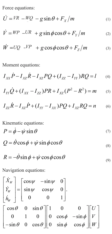
Force equations:

m

F

g

W

Q

V

R

U

sin

T

_X

(1)

m

F

g

U

R

W

P

V

sin

I

cos

T

_Y

(2)

m

F

g

V

P

U

Q

W

cos

I

cos

T

Z G

Moment equations:

(

)

XX XZ XZ ZZ YY

I

P

I

R

I

PQ

I

RQ

l

(4)

2 2

(

)

(

)

YY XX ZZ XZ

I Q

I

PR

I

P

R

m

K

(

)

ZZ XZ YY XX XZ

I R

I P

I

PQ

I RQ

n

(6)

Kinematic equations:

T

\

I

sin

P

(7)

T

I

\

I

T

cos

sin

cos

Q

₍₈₎

T

I

\

I

T

sin

cos

R

₍₉₎

Navigation equations:

cos

sin

0 sin

cos

0 .

0

1 cos

0 sin

1

0

1

0

0 cos

sin

0 cos

0 sin

cos

W

X

Y

h

U

V

W

\

T

I

T

I

ª

º

_ª

_º

«

_{» «}

_»

«

_{» «}

_»

«

_{» «}

_¬

_»

_¼

¬

¼

ª

º ª

º ª º

«

» «

» « »

«

» «

» « »

«

» «

» « »

¬

¼ ¬

¼ ¬ ¼

VR WQ

WP UR

(4)

48 M. Mortazavi , A. Askari

The forces and moments are:

X X A engine X JATO

F

(11)

Y Y A Y JATO

F

(12)

Z Z A Z JATO

F

G

JATO

A

l

(14)

JATO engine

A

m

K

A JATO

n

(16)

Engine forces, torque and gyroscopic effect as well as environmental forces such as wind shear can have any-$#%&'###% %&?%##@G^; %7?"#%%7'-tions are made. Engine thrust is limited to the X-axis located above the aircraft center line that makes m_Thrust and no calculations are made for the gyroscopic effect #>&@GK^;

Aerodynamic Model

The terms F_AX, F_AY and F_AZ represent the resultant aerodynamic forces.

sin

cos

sin

X A F

F

L

D

S

E

(17)

cos

Y A F

F

S

E

(18)

cos

sin

Z A

F

L

D

(19)

*%&<%#'%#& sideforce are calculated as follows:

S

q

V

C

2 V

c

C

2 V

c

q

C

L

2

L L

q L L

L0

e

»

¼

º

«

¬

ª

»

¼

º

«

¬

ª

'

W H W

W

G D

D

(20)

(21)

S

q

)

(C

S

F Y_E

C

Y_G_r

G

r

(22)

The aerodynamic moments represent the torque about the center of mass of the aircraft and are determined in the following equations:

R

l l

A

l l l

b

C

2V

l

qSb

b

C R

2V

P

a r

P

C

a C

r

E

G G

W

E

G

ª

º

«

»

«

»

«

»

«

»

¬

¼

(24)

e

mo mq

2 A

m

c

C

C q

2V

m

qSc

V

c

C

2V

V

m

D

D G

W

W H

W W

D

ª

º

«

»

«

»

«

_ª

_'

_º

»

«

_«

_»

»

«

_¬

_¼

»

¬

¼

BK

R

n n

A n

b

C

2V

n

qSb

b

C R

2V

P

a r

n n

P

C

a C

r

E

G G

W

E

G

ª

º

«

»

«

»

«

»

«

»

¬

¼

(26)

UAV Characteristics

The UAV characteristics are shown in table 1 [8].

Item Nomenclature Quantity 1 External Dimensions

1.1 Wing Span G

1.2 Wing Aspect Ratio 4 ;G Mean Aerodynamic Chord 0.8 m 1.4 Fuselage Length K;K ;K Fuselage Diameter 0.42 m 1.6 Wing Area B;BK2

1.7 C.G. Position From Nose G;G 2 Weight

2.1 Gross Weight HBK& 2.2 Launch Weight HK& G Aerodynamic

G; Wing Lift Curve Slope 0.068 /rad

G;B ##' ;K

G;G Horizontal L.C.S. 0.062 /rad G;H Vertical L.C.S 0.062 /rad 4 Performance

4.1 ISA Condition

4.2 Stall Speed 70 m/s H;G Engine Thrust GK

(5)

49

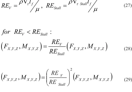
Aerodynamic Forces and Moments Correction

The idea used in this research for the aerodynamic forc-es and moments in low a Reynolds number, is to consid-er a linear and quadratic relation between Reynolds and Aerodynamic forces and moments as below:

V

,

Stall f

f

V Stall

l

RE

U

W

_P

RE

U

W

_P

(27)

, , , ,

:

,

V Stall

V

X Y Z X Y Z X Y Z X Y Z

Stall

for RE

RE

F

M

F

M

RE

(28)

XYZ XYZ

Stall V Z

Y X Z Y

X F M

RE RE M

F _, _, _, _,

2 ,

, ,

, , ,

¸¸¹ · ¨¨©

§

(29)

where F_X,Y,Z and M_X,Y,Z are the forces and moments in equations 11 to 16.

JATO Model

& G %$% +| % ; +| thrust is as follows:

cos(

)

X JATO JATO JATO

F

T

D

G

0

Y JATO

F

G

sin(

)

Z JATO JATO JATO

F

T

D

GB

Figure 3. JATO thrust model

JATO Installation on the UAV

Figure 4 shows the schematic installation of the JATO

*+3; %& _JATO, causes an instability

behavior and decreasing it, causes the UAV not to reach a proper altitude. Obviously, the JATO thrust line must pass through the cg _(UAV+JATO).

Figure 4. JATO location on the UAV

Misalignment of JATO Thrust

Ideally, there is no misalignment in JATO thrust, but actually JATO thrust line is not on the JATO longitu-dinal axis.

Asymmetric Forces and moments acting on the UAV when JATO thrust is aligned to right side are:

(MJT: Misalignment of JATO Thrust)

.

cos(

)

Long JATO JATO MJT

T

D

GG

sin(

)

Lateral JATO JATO MJT

T

D

GH

.

cos(

)

X MJT Long JATO JATO

F

T

D

GK

Y MJT Lateral JATO

F

T

G\

.

sin(

)

Z MJT Long JATO JATO

F

T

D

G

(

)

(

)

MJT X MJT cg V JATO nose

Z MJT cg V JATO nose

m

F

X

F

Z

G

(

)

MJT Y MJT cg V JATO nose

n

F

X

G

(

)

MJT Y MJT cg V JATO nose

l

F

Z

(40)

Unsimultaneous Cut of Pins

*+3%="$7%'&-K;+|%%7% the UAV separates from the launcher. It is necessary to check the UAV behavior when pins do not cut simulta-neously.

(6)

K M. Mortazavi , A. Askari

Figure 5. UAV connection to launcher (F_z is perpendicular and toward the page)

Where the left pin cut, forces and moments acting on the UAV are:

(UCP: Unsimultaneous Cut of Pins)

X UCP X MJT engine

F

(41)

Y UCP Y MJT

F

(42)

Z UCP Z MJT

F

HG

(

)

(

)

UCP X UCP cg V pin

Z UCP cg V pin

m

F

Z

F

X

(44)

(

2)

(

)

UCP X UCP f Y UCP cg V pin

n

F

d

F

X

HK

(

2)

(

)

UCP Z UCP f Y UCP cg V pin

l

F

d

F

Z

(46)

Total JATO forces and moments acting on the UAV are

X JATO X MJT X UCP

F

(47)

Y JATO Y MJT Y UCP

F

(48)

Z JATO Z MJT Z UCP

F

(49)

JATO MJT UCP

m

K

JATO MJT UCP

n

K

JATO MJT UCP

l

KB

Center of Gravity and Moment of Inertia

+ '% " %"% % *+3 +| # +|#%'%%#+|% separated from UAV. The variable cg position is:

t₁<Time<t₂:

JATO UAV

cg JATO cg

UAV cg

M

r

M

r

M

r

UAV JATO

Var

K

KG

Time=t₂:

UAV JATO Case Var

UAV cg JATO Case cg

cg

UAV JATO Case

M

r

M

r

M

K

KH

Time>t₂ :

UAV Var cg

cg

r

K

KK

Change of weight and moment of inertia of the system (UAV+JATO) during JATO burning are considered in the simulation.

Because of changing the cg location, the correction on #'%%

( )

[(

)

]

m UAV JATO m UAV

L UAV cg UAV JATO cg UAV ac

C

X

K\

+'%₁ and cg position move back, causing a

decrease in the stability margin that must be considered in the analysis.

(7)

K

Results and Discussions

Case Studies

Three case studies of launch simulation of the UAV are presented. All of the case studies involve two control

%#% _e _a that may be changed by operator and/

7%;'% test launch is without engine and the second and third tests are launched with engine.

Measurement devices are vertical gyro, GPS receiver, barometric altimeter and telecommunication apparatus. All these devices were calibrated and have been used before on the other UAVs. Measurement parameters are pitch angle, bank angle, altitude, pressure altitude, tem-perature, latitude, longitude, and ground speed. Note #!"#&%&%; This fact causes some data loss and decreases the preci-sion of the test data in comparison with the simulation result. Because of this, the simulation and test results can be compared in large scale.

Case Study I: Launch Test without Engine

The UAV weight is 420 kg and JATO produces 24 KN in average during t₂-t₁=2.2 seconds. The simulations and

&%%%"%-_JATO=10.670

0=20

0_7`+

eK 0_,t

1=0.

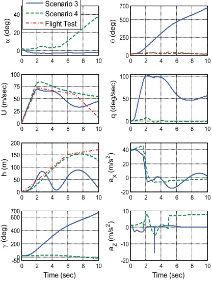
To show the correction factor which is considered in equations 27 and 29, four scenarios are considered as below:

Scenario 1: simulation of the launch phase consider-ing the quadratic correction factor

(

R

E

_V

R

E

_Stall

)

2

in equation 29.

Scenario 2: simulation of the launch phase considering the linear correction factor

(

R

E

_V

R

E

_Stall

)

in equation 28.

`G%#7%$-sidering correction factor

(

R

E

_V

R

E

_Stall

)

in equation 28.

Scenario 4: simulation of the launch phase considering zero forces and moments for

R

E

_V

R

E

_Stall.

`#%B%$'&\; There is a good agreement in altitude between scenario & %; = K 7 % =$ % & % =G7=$%B& test. Therefore, it can be concluded that considering the quadratic form of the correction factor for forces and moments (equation 29) is more accurate than the linear model (equation 28). Figure 7 shows simulation # % G H; ` G % 7= =-cause pitch angle and altitude are not in their reasonable range. Although scenario 4 looks acceptable, there is an #=BK7=$%%-&%;

0 2 4 6 8 10

0 2.5 5

D

(

deg)

0 2 4 6 8 10

0 20 40

T

(

deg)

Scenario 1 Scenario 2 Flight Test

0 2 4 6 8 10

0 25 50 75 100

U

(

m

/se

c)

0 2 4 6 8 10

-10 0 10

q (

deg/

s

e

c

)

0 2 4 6 8 10

0 50 100 150 200

h

(m)

0 2 4 6 8 10

0 20 40

aX

(m/

s

2)

0 2 4 6 8 10

-10 0 10 20 30

Time (sec)

J

(

deg)

0 2 4 6 8 10

-10 0 10

Time (sec)

aZ

(m/

s

2)

Figure 6. Simulation of the UAV – Scenario 1,2

0 2 4 6 8 10

0 20 40

D

(

deg)

0 2 4 6 8 10

0 250 500 700

T

(

deg)

Scenario 3 Scenario 4 Flight Test

0 2 4 6 8 10

0 25 50 75 100

U

(

m

/se

c)

0 2 4 6 8 10

0 50 100

q (

deg/

s

e

c

)

0 2 4 6 8 10

0 50 100 150 200

h

(m)

0 2 4 6 8 10

-20 0 20 40

aX

(m/

s

2)

0 2 4 6 8 10

-500 200 400 600 700

Time (sec)

J

(

deg)

0 2 4 6 8 10

-20 -10 0 10

Time (sec) aZ

(m/

s

2)

Figure 7. Simulation of the UAV – Scenario 3,4

RE RE

(8)

KB M. Mortazavi , A. Askari

&%$%%&%#*+3; %=K7\7 error in velocity that shows a good agreement. Differ-ences in speed after t=7 seconds can be because of some 7=% #& # '% 7"7; #&#'%&-er than is the one consid#&#'%&-ered in the simulation. Anoth#&#'%&-er effect is because of lateral oscillation that causes loss of UAV energy and reduces speed to lower than the point predicted in the simulation.

&=&'&## simulation and test. It seems a pilot command after t=4

seconds in G_E;`'%%'&;

Also, during JATO burning, the bank angle increases to G0_{. Using simulation, it is concluded that this occurs}

because of both JATO misalignment in xy-plane and non-simultaneous cut of pins (D_MJT=0.010_,'_t

UCP=0.01

sec).

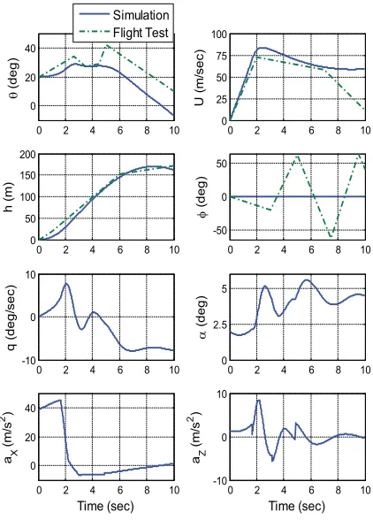
Although speculating what the pilot may have thought %#'$%#%%%%;& 9 illustrates simulation of the test using an unstable au-7&%%¡?; gain of bank attitude hold mode is deliberately select-ed as K_¢B¢_Comm.=00_{. Figure 9 does not resemble}

what happened in the real test. The bank angle grad-ually increases during 10 seconds and the maximum

7 % = BK0_{;two points which are different}

from the test. Another assumption is the pilot’s reaction to hold the bank angle near zero. Figure 10 illustrates %#*+3$77;'& shows a similarity between the simulation and the test. Therefore, it is concluded that the pilot tried to stabilize the UAV in longitudinal and lateral-directional modes.

As a result, because the UAV has a high acceleration during launch, pilot commands cause an instability =%&&%%%&& system. Figure 11 shows the UAV can be effectively controled with a stable gain autopilot which is shown in

'&B¤_¢;K;

0 2 4 6 8 10

0 20 40

T

(

deg)

0 2 4 6 8 10

0 25 50 75 100

U

(

m

/se

c)

Simulation Flight Test

0 2 4 6 8 10

0 50 100 150 200

h

(m)

0 2 4 6 8 10

-50 0 50

I

(

deg)

0 2 4 6 8 10

-10 0 10

q (

deg/

s

e

c

)

0 2 4 6 8 10

0 2.5 5

D

(

deg)

0 2 4 6 8 10

0 20 40

Time (sec) a X

(m/

s

2)

0 2 4 6 8 10

-10 0 10

Time (sec) aZ

(m/

s

2)

0 2 4 6 8 10

0 20 40

T

(

deg)

0 2 4 6 8 10

0 25 50 75 100

U

(

m

/se

c)

0 2 4 6 8 10

-10 0 10

q (

deg/

s

e

c

)

0 2 4 6 8 10

0 50 100 150 200

h

(m)

0 2 4 6 8 10

-50 0 50

I

(

deg)

0 2 4 6 8 10

-2 0 2 4 6

\

(

deg/

s

e

c

)

0 2 4 6 8 10

-200 -100 0 100 200

Time (sec)

p (

deg/

s

e

c

)

0 2 4 6 8 10

-10 -5 0 5 10

Time (sec)

r (

deg/

s

e

c

)

Figure 9. Simulation of the UAV

(9)

KG

0 2 4 6 8 10

0 10 20 30 40 50

T

(

deg)

Simulation Flght Test

0 2 4 6 8 10

0 25 50 75 100

U

(

m

/se

c)

0 2 4 6 8 10

-10 0 10 20

q (

deg/

s

e

c

)

0 2 4 6 8 10

0 50 100 150 200

h

(m)

0 2 4 6 8 10

-50 0 50

I

(

deg)

0 2 4 6 8 10

-5 0 5 10 15

\

(

deg/

s

e

c

)

0 2 4 6 8 10

-50 0 50

Time (sec)

p (

deg/

s

e

c

)

0 2 4 6 8 10

-10 -5 0 5 10

Time (sec)

r (

deg/

s

e

c

)

Figure 10. Simulation of the UAV Using operator command

0 2 4 6 8 10

0 20 40

T

(

deg)

0 2 4 6 8 10

0 25 50 75 100

U

(

m

/se

c)

0 2 4 6 8 10

-10 0 10

q (

deg/

s

e

c

)

0 2 4 6 8 10

0 50 100 150 200

h

(m)

0 2 4 6 8 10

-50 0 50

I

(

deg)

0 2 4 6 8 10

-2 0 2 4 6

\

(

deg/

s

e

c

)

0 2 4 6 8 10

-10 0 10 20

Time (sec)

p (

deg/

s

e

c

)

0 2 4 6 8 10

-5 0 5

Time (sec)

r (

deg/

s

e

c

)

Figure 11. Simulation of the UAV Using autopilot command with a stable gain (K!=0.2)

UAV f(u)

Gyro

f(u) Gain

K _phi From

[phi _Comm ]

Aileron Actuator A_demand A_actual

Figure 12. Roll Attitude Hold/Select Mode autopilot

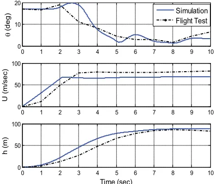
Case Study II: Launch Test with Engine

In this test, the prototype has an engine that produces a %#=G¤;*+3$&%B&¥$ is the empty weight. The JATO thrust is 11700 N during

t₂-t₁B;B%%;`&%%

%"%_JATOK;K0

0=20 0_,

7`+ _{e 0}=100_,t

1=0.

&G%%%&

test of the UAV. Lateral-directional parameters are near zero and ignorable. The difference between t₂ in simula-tion and test is due to the difference in the burning time of the JATO ideal and actual models used for simulation and test, respectively. The difference between t₂ in the simulation and the test is due to difference in the burn-ing time of JATO considered in ideal and actual models for simulation and test, respectively. Like case study I, due to pilot command during t=2 and t=4 seconds, cause pitch angle is lower than that in the simulation. Therefore, velocity in the simulation is lower than the %; '& % = 7 which is acceptable.

0 1 2 3 4 5 6 7 8 9 10

0 10 20

T

(

deg)

0 1 2 3 4 5 6 7 8 9 10

0 50 100

U

(

m

/se

c)

0 1 2 3 4 5 6 7 8 9 10

0 50 100

Time (sec)

h

(m)

(10)

KH M. Mortazavi , A. Askari

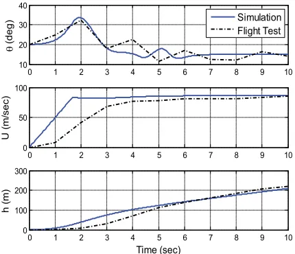
Case Study III: Launch Test in The Presence of Headwind

The UAV weight is 420 kg and JATO averagely pro-duces 24 KN during t₂-t₁=2.2 sec. In the test, there is a $!G;77%% the UAV in the presence of headwind. The simulation

&%%%"%-_JATO=11.60

0=20

0_7`+

e 0=10 0_{, t}

1=0.

& H %% & % % # UAV. Because of headwind, the pitch angle increases

about 120_{% %; '& %}

good agreement of the pitch angle in the simulation and %;+#G%%77%7 the pitch angle equal to T_Command K0_.

0 1 2 3 4 5 6 7 8 9 10

10 20 30 40

T

(

deg)

0 1 2 3 4 5 6 7 8 9 10

0 50 100

U

(

m

/se

c)

0 1 2 3 4 5 6 7 8 9 10

0 100 200 300

Time (sec)

h

(m)

"# $ of headwind=30 km/h

As discussed in case study II, because the impulses in JATO ideal and actual models are equal and burning %##%=%'&H "##'%="=-come equal after 10 seconds.

In this test, by removing some problems existing in the last two tests like pilot command or an accurate pro-totype, there are no differences between simulation and test after 10 seconds.

Sensitivity Analysis

%%%%$%&'"%-tion and, therefore, it is possible to use this simula%%%%$%&'"%-tion as a design tool and in sensitivity analysis in order to measure the sensitivity of the UAV variables to

param-eter variation in the launch phase. Actually, it helps

de-%&&7%%%_JATO, T₀, JATO

thrust and duration (T_JATO, t_JATO), maximum 't_UCP and

maximum D_MJT; % % & %

cost.

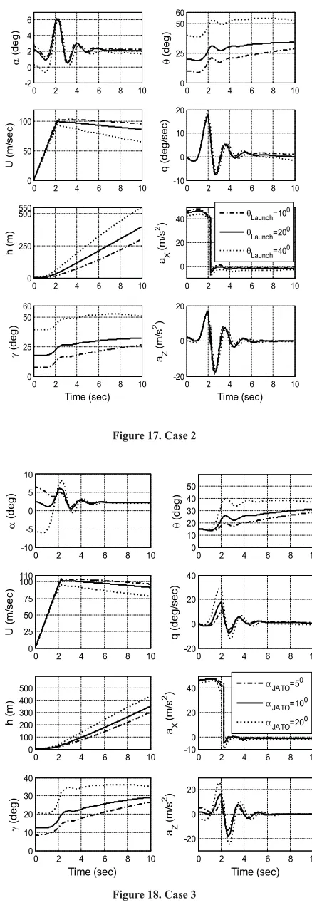
Table 2 includes different JATOs with similar impuls-es, different launch angles (T₀), JATO angles (D₀), JATO misalignment and non-simultaneous cuts of pins. The initial data is: T_JATOBK¤₂=2.2 sec, T₀=200_,D

0=10 0_,

Ge0K

0_[7].

Case TJATO

KN tJATO

sec

Imp.

KN.s T

deg

DJATO

deg 'DJATO

deg 'tPins

sec

1 KK BK

G; 1, 2.2,

4

KK 200 ₁₀0 ₀ ₀

2 BK 2.2 KK

100_,

200_,

400

100 ₀ ₀

G BK 2.2 KK K0

K0_,

100_,

200

0 0

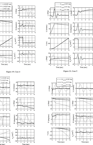
4 BK 2.2 KK 200 ₁₀0

.001, .01,

.1

0

K BK 2.2 KK 200 ₁₀0 ₀

.001,

.01, .1

Table 2. Case studies for the launch - Ge0=5 0

The case studies of launch phase simulation of differ-7%%7''&%KBB;& K % +| % $ % -pulse used for launch. Figure 16 shows using JATO with

T_JATOK ¤ %% %=" +| $

T_JATOG;K¤%%'&\;+

%&₀) causes decrease in the

velocity that may be lower than the stall speed. Con-versely, decreasing it causes a decrease in the altitude,

%=%'&;&%$%&_JATO

%% & # & '% $ %-onds and the stability of the UAV. On the contrary, low _JATO decreases altitude, which is not enough for recov-"&"%;%"'&% and 20 illustrate the maximum time difference between

7 % % ? ;K % ¦_Pins§;K %;

#¦_Pins¨;K % *+3 & = %= =

longitudinal and lateral-directional modes. Similarly,

=%'&%BBB?+|%-& % ? ;K0_¦

Unsymmetric§;K 0_),

(11)

KK

0 0.5 1 1.5 2 2.5 3 3.5 4 4.5 5

0 1 2 3 4 5 6x 10

4 Time (sec) TJAT O (J A T O T h ru s t) (N ) T

JATO=55 KN,tJATO=1 sec T

JATO=25 KN,tJATO=2.2 sec T_JATO=13.75 KN,t_JATO=4 sec

Figure 15. Case 1

0 2 4 6 8 10

-5 0 5 10 15 D ( deg)

0 2 4 6 8 10

0 10 20 30 40 50 T ( deg)

0 2 4 6 8 10

0 50 100 120 U ( m /se c)

0 2 4 6 8 10

-20 0 20 40 q ( deg/ s e c )

0 2 4 6 8 10

0 100 200 300 400 500 h (m)

0 2 4 6 8 10

0 50 100 ax (m/ s 2)

0 2 4 6 8 10

0 10 20 30 40 Time (sec) J ( deg)

0 2 4 6 8 10

-20 0 20 40 60 Time (sec) az (m/ s 2)

T_JATO=55 KN,t_JATO=1 sec T_JATO=25 KN,t_JATO=2.2 sec T

JATO=13.75 KN,tJATO=4 sec

0 2 4 6 8 10

-2 0 2 4 6 D ( deg)

0 2 4 6 8 10

0 25 50 60 T ( deg)

0 2 4 6 8 10

0 50 100 U ( m /se c)

0 2 4 6 8 10

-10 0 10 20 q ( deg/ s e c )

0 2 4 6 8 10

0 250 500 550 h (m)

0 2 4 6 8 10

0 20 40 aX (m/ s 2)

0 2 4 6 8 10

0 25 50 60 Time (sec) J ( deg)

0 2 4 6 8 10

-20 0 20 Time (sec) a Z (m/ s 2)

TLaunch=10 0

TLaunch=20 0

TLaunch=40 0

0 2 4 6 8 10

-10 -5 0 5 10 D ( deg)

0 2 4 6 8 10

0 10 20 30 40 50 T ( deg)

0 2 4 6 8 10

0 25 50 75 100 110 U ( m /se c)

0 2 4 6 8 10

-20 0 20 40 q ( deg/ s e c )

0 2 4 6 8 10

0 100 200 300 400 500 h (m)

0 2 4 6 8 10

0 20 40 -10 aX (m/ s 2 )

0 2 4 6 8 10

0 10 20 30 40 Time (sec) J ( deg)

0 2 4 6 8 10

-20 0 20 Time (sec) aZ (m/ s 2 )

DJATO=5 0

DJATO=10 0

DJATO=20 0

(12)

K\ M. Mortazavi , A. Askari

0 2 4 6 8 10

-100 -50 0 50 100 D ( deg)

G t=0.001 sec

G t=0.01 sec

G t=0.1 sec

0 2 4 6 8 10

-20 0 20 40 60 T ( deg)

0 2 4 6 8 10

0 50 100 U ( m /se c)

0 2 4 6 8 10

-50 -25 0 25 50 Q ( deg/ s e c )

0 2 4 6 8 10

0 250 500

h

(m)

0 2 4 6 8 10

-20 0 20 40 60 ax (m/ s 2)

0 2 4 6 8 10

-50 0 50 100 Time (sec) J ( deg)

0 2 4 6 8 10

-200 -100 0 100 Time (sec) az (m/ s 2)

0 2 4 6 8 10

-20 0 20 E ( deg)

G t=0.001 sec

G t=0.01 sec

G t=0.1 sec

0 2 4 6 8 10

-40 -20 0 20 V ( m /se s)

0 2 4 6 8 10

-600 -400 -200 0 I ( deg)

0 2 4 6 8 10

-20 0 20 40 \ ( deg)

0 2 4 6 8 10

-400 -200 0 200 P ( deg/ s e c )

0 2 4 6 8 10

0 20 40 R ( deg/ s e c )

0 2 4 6 8 10

-100 0 100 200 Time (sec) Y (m)

0 2 4 6 8 10

-100 0 100 200 300 Time (sec) ay (m/ s 2)

0 2 4 6 8 10

0 2 4 6 D ( deg)

GD_JATO=0.001 deg

GD_JATO=0.01 deg

GD_JATO=0.1 deg

0 2 4 6 8 10

20 40 30 T ( deg)

0 2 4 6 8 10

0 50 100 U ( m /se c)

0 2 4 6 8 10

-10 0 10 20 Q ( deg/ s e c )

0 2 4 6 8 10

0 200 400

h

(m)

0 2 4 6 8 10

0 20 40 ax (m/ s 2)

0 2 4 6 8 10

-50 0 50 100 Time (sec) J ( deg)

0 2 4 6 8 10

-20 0 20 Time (sec) az (m/ s 2)

0 2 4 6 8 10

-1 0 1 E ( deg)

GD_JATO=0.001 deg

GD_JATO=0.01 deg

GDJATO=0.1 deg

0 2 4 6 8 10

-2 0 2 V ( m /se s)

0 2 4 6 8 10

-30 -20 -10 0 I ( deg)

0 2 4 6 8 10

-30 -20 -10 0 \ ( deg)

0 2 4 6 8 10

-10 -5 0 P ( deg/ s e c )

0 2 4 6 8 10

-3 -2 -1 0 1 R ( deg/ s e c )

0 2 4 6 8 10

-150 -100 -50 0 Time (sec) Y (m)

0 2 4 6 8 10

-2 0 2 Time (sec) ay (m/ s 2)

(13)

K

Conclusions

In this paper, the simulation of UAV in the launch phase $ % %7' 7=% # % 7% $% -oped. Accurate formulation of symmetric and asym-metric forces and moments acting on the UAV offered additional insight and understanding, which could not have been gained without simulation. Three case stud-ies were modest examples of this simulation. Compar-ison of simulation and test in asymmetric condition, in conjunction with headwind and the UAV with and with-out engine showed an acceptable agreement between %%%%&'"% $%';$%%7$*+3 would behave in these conditions and how to decide whether it is safe to launch the UAV.

The key in solving this problem was to recognize the contribution of aerodynamic forces and moments, JATO forces and moments in symmetric and asymmet-ric conditions, cg traveling during launch and moment #'%=%#&&;

Sensitivity analysis was shown as a useful tool to de-sign launch parameters. It increased the insight of the launch performance as a result of effective parameters in the launch phase. For developing the research, some measures can be done such as extending and imple-& imple-& '" % %imple-& 7-timization algorithm to design the launch parameters which are quantitatively more precise.

Acknowledge

The authors hereby express their gratitude for the grant support from the HESA design bureau.

References

1. Johnson, Eric N., Fontaine,Sebastiene, “Use of

Flight Simulation to Complement Flight Testing #$<%*+3%+++B<HKB; 2. Brian L. Stevens & Frank L. Lewis, Aircraft

Con-trol and Simulation, John Willey & Sons INC, (1992).

G; Roskam, Jan, Airplane Flight Dynamics and Au-tomatic Flight Controls, Jan Roskam, Kansas, (1997).

4. Louise V. Schmidt, “Introduction to Aircraft Flight Dynamis”, AIAA, 1998.

K; Cooke, Joseph M., Zyda, Michael J., Pratt, David R., McGhee, Robert B., NPSNET: “Flight Simu-lation Dynamic Modeling Using Quaternion”, In Presence, Vol. 1, No. 4, pp. 404-420, 1994. 6. Ralston, John, Kay, Jacob, “The Utilization of

High Fidelity Simulation in the Support of High Angle of Attack Flight Testing”, Hampton, VA BG\\\*`+;

7. Mortazavi, Mahdi, Askari, Abdorreza, “Simula-tion of RPV’s launch phase”, The forth biennial conference of the Iranian aerospace society Con-ference, Amirkabir University of Technology, BG;

(14)