Vol 4, No. 2, (2014), pp 57-72
A new approach for solving nonlinear
system of equations using Newton
method and HAM
J. Izadian∗, R. Abrishami and M. Jalili
Abstract
A new approach utilizing Newton Method and Homotopy Analysis Method (HAM) is proposed for solving nonlinear system of equations. Accelerating the rate of convergence of HAM, and obtaining a global quadratic rate of convergence are the main purposes of this approach. The numerical results demonstrate the efficiency and the performance of proposed approach. The comparison with conventional homotopy method, Newton Method and HAM shows the great freedom of selecting the initial guess, in this approach.
Keywords: Homotopy Analysis Method; Zero order deformation equations; Control convergence parameter; Newton’s method; Iterative method; Multi-step iterative method; Order of convergence.
1 Introduction
Solving algebraic and transcendental equations is an interesting mathemat-ical problem that has been occupied an important place in mathematmathemat-ical history. This problem arises in different applications of mathematics in sci-ences and engineering. Analytical solution of this problem is reserved to a small category of equations. For this reason and the exigencies of those increasing applications, from the beginning of era of electronic computing numerical methods of these problems have been progressed.
∗Corresponding author
Received 21 February 2014; revised 27 July 2014; accepted 13 August 2014 J. Izadian
Department of Mathematics, Faculty of Sciences, Mashhad Branch, Islamic Azad Univer-sity, Mashhad, Iran. e-mail: Jalal [email protected]
R. Abrishami
Department of Mathematics, Faculty of Sciences, Mashhad Branch, Islamic Azad Univer-sity, Mashhad, Iran
M. Jalili
Department of Mathematics, Neyshabur Branch, Islamic Azad University, Neyshabur, Iran.
Actually there is a vast group of conventional methods to solve algebraic and transcendental equations, but yet there exist enormous difficulty due to local convergence of these methods that make the new research inevitable. Particular numerical solution of system of nonlinear equations is realized by different methods. A traditional method is Newton method that can have quadratic order of convergence, but the convergence is local [16]. There is a variety of modified Newton methods which make a global convergence possible [16]. Many new one-step and multi-step methods are used to solve these system of equations (for more details one can refer to [4, 7, 8]). There is also acceleration methods and multi-step methods but these methods are also very dependent to initial guess and have local convergence in the most of the cases [16]. Recently the homotopy method using the notion of homotopy and functional series are applied to solve the system of nonlinear equations [1, 3, 6, 15, 11, 17]. Some methods are very suitable, but in practice they need to solve a system of differential equations with initial conditions [14]. One of the most important of Homotopy methods which is principally used for solving the nonlinear differential equations is Homotopy Analysis Method (HAM), that can be applied for solving nonlinear equations, but it is normally slow with local convergence [14]. In this paper a combination of Newton Method and HAM is considered to solve the algebraic and transcendental system of equations with the aim of improving the both mentioned methods, in view of local convergence and the rate of convergence. The results of proposed method will be compared with other methods.
The organization of the paper is as follows. In Section 2 a concise descrip-tion of the Newton Method, the Homotopy Method are presented. In Secdescrip-tion 3 the fundamental of HAM and proposed approach is discussed. In Section 4 the numerical results for 3 methods are given and compared. Finally Section 5 ends the paper with conclusion and discussion.
2 Description of problem and the methods
Consider the following nonlinear algebraic or transcendental system of equa-tions
F(x) = 0 , F = (f1, f2,· · ·, fn), (1)
where F : D ⊂Rn →Rn, that D is an open region in Rn andF ∈ C1(D) such thatF(bx) = 0. The vectorbxis called the zero ofFor the solution of the equation (1). Recalling that the Newton Method for solving (1) is formulated as follows
x(k+1)=x(k)−[DF(x(k))]−1F(x(k)), k= 0,1,2,· · · , (2)
differentiable functions. In general, the rate of convergence is quadratic in a neighborhood of the solutionbx, with local convergence property. As a second choice for solving (1), the homotopy method for the system of nonlinear equation is recalled [6]. The Homotopy function
H: [0,1]×Rn →Rn ,
is defined by
H(q,x) =qF(x) + (1−q)(F(x)−F(x(0))) (3) =F(x) + (q−1)F(x(0)), (4)
here x(0) is an initial guess of bx and q is called Homotopy parameter or embedding parameter. Obviously, atq= 0 andq= 1,
H(0,x) =F(x)−F(x(0)), H(1,x) =F(x).
Ifqincreases from 0 to 1 then the functionH(q,x) varies continuously from
F(x)−F(x(0)) to F(x). In topology, such a kind of continuous variation is called deformation. The function H respect to parameter q, provides us a family of functions that can lead from the known value x(0), to solution
b
x. The function H is a Homotopy between H(0,x) = F(x)−F(x(0)) and H(1,x) =F(x). Accepting thatϕ: [0,1]→Rn,x=ϕ(q) is a unique solution of the equation
H(q,x) = 0, q∈[0,1], (5)
or
H(q, ϕ(q)) = 0, q∈[0,1]. (6) The set{ϕ(q)|0≤q≤1} can be viewed as a family of parameterized curves respect toqinRn fromϕ(0) toϕ(1) =x. The solutionb bxofF(x) = 0 can be
obtained by solving the following system of equations
ϕ′(q) =−[J(ϕ(q))]−1F(ϕ(0)), 0≤q≤1,
with the initial conditionϕ(0) =x(0), whereJ(ϕ(q)) is jacobian matrix ofH respect to x[6]. This method will be reffered as HM.
3 HAM combined with Newton method
The Homotopy Analysis Method (HAM) is proposed by Liao [2]. In this method one introduces a homotopy function for solving (1). To be more precise, the following homotopy function is considered:
where q∈[0,1] is an embedding parameter andϕ(q) is a function of q, and x(0) ∈ Rn is an initial estimation of bx, the solution of (1). Also, N is a
nonlinear operator andLis a linear operator and
N(x)≡F(x). (8)
Ifq= 0 and q= 1, then consideringϕ(0) =x(0), yields
H[q, ϕ(q)]q=0=L[ϕ(0)−x(0)] = 0, (9)
and
H[q, ϕ(q)]q=1=N[ϕ(1)], ϕ(1) =bx.
By using (9), the vector
ϕ(1) =bx,
is obviously the solution of the equation
H[q, ϕ(q)]q=1= 0 .
As the embedding parameter q increases from 0 to 1, the solution ϕ(q) of equation
H[q, ϕ(q)] = 0,
depends upon the embedding parameterqand varies from initial approxima-tionx(0)to the solutionxbof equation (9). Now by using homotopy function (7) we construct a family of equations
(1−q)L[ϕ(q)−x(0)] =qN(ϕ(q)), q∈[0,1], (10)
subject to the initial condition
ϕ(0) =x(0) . (11)
Consider equation (1) and letA be a non-singular matrix which will be determined later. We construct following deformation equation that is called zeroth-order deformation equation:
(1−q)A(ϕ(q)−x(0)) =qF(ϕ(q)). (12)
Supposexbis solution ofF(x) = 0 and the sequence
{
x(i)
}
i∈N
exist with the
following property
b
x=
∞ ∑
m=0 x(m) ,
and
Next a functionϕ: [0,1]→Rn is defined as follows
x=ϕ(q) =
∞ ∑
m=0
x(m)qn , q∈[0,1],
Subject to
ϕ(0) =x(0) , (13)
ϕ(1) =bx. (14)
By differentiating (12) with respect toq, the following equation is obtained:
−A(ϕ(q)−x(0)) + (1−q)(A d
dqϕ(q)) =F(ϕ(q)) +q d
dqF(ϕ(q)). (15)
Puttingq= 0 in (15) yields
Ad
dqϕ(q)
q=0
=F(ϕ(0)). (16)
MatrixAbeing non-singular, it deduces
d dqϕ(q)
q=0
=A−1F(ϕ(0)). (17)
On the other hand,
d dqϕ(q) =
∞ ∑
m=1
mx(m)qm−1.
Then
d dqϕ(q)
q=0
=x(1)=A−1F(x(0)). (18)
The equation of (15) is called first-order deformation equation. By differen-tiating equation (15) with respect toq, the following equation is obtained
−2A d
dqϕ(q) + (1−q)A d2
dq2ϕ(q)
= 2d
dqF(ϕ(q)) +q d2
dq2F(ϕ(q)). (19)
Puttingq= 0, the second-order deformation equation is obtained as follows
−2Ax(1)+ 2Ax(2)= 2DxF(x(0))x(1) , (20)
or
By repeating the same procedure the m-th order deformation equation can be obtained. Indeed, the following proposition can be proved.
Proposition 3.1. If F : Rn → Rn, and F ∈ Cm(Rn), A ∈Rn×n a given matrix, and
x=ϕ(q) =
∞ ∑
m=0
x(m)qm, ϕ: [0,1]→Rn ,
(1−q)A(ϕ(q)−x(0)) =qF(ϕ(q)).
whereϕ is an analytic function, then
A(x(m)−χmx(m−1)) =
1 (m−1)!
dm−1
dqm−1F(ϕ(q))
q=0
, (21)
where
χm=
{
0 m≤1
1 o.w. .
If m≥2 andAbe a nonsingular matrix then
x(m)=x(m−1)+ 1 (m−1)!A
−1 dm−1
dqm−1F(ϕ(q,x))
q=0
. (22)
The equation (22) is called m-th order deformation equation.
For solving system of algebraic equations in general one can use the above equations to determine the vectorial terms x(i) of xb = ∑∞
i=0x
(i), i.e. the following equations.
x(m)=
x(0) m= 0
A−1F(x(0)) m= 1
x(m−1)+ 1 (m−1)!A−
1dm−1
dqm−1F(ϕ(q))
q=0
m≥2
. (23)
In practice, one can obtain a finite number of x(i). Then by considering partial sum of above series one can determineϕ(1) approximately by a Kth
order partial sum as follows:
b
x=ϕ(1)≈x(0)+x(1)+· · ·+x(K) ,
ϕ(q) =
∞ ∑
m=0
x(m)qm,
may be divergent atq= 1. To overcome this restriction, Liao [14] introduced an auxiliary parameter h̸= 0 to construct a kind of deformation equations based on
(1−q)A(ϕ(q, h)−x(0)) =qhF(ϕ(q, h)),
where
ϕ(q, h) =
∞ ∑
m=0
x(m)(h)qm,
the vectorsx(m)are dependent onh. In particular if series is convergent for at least onebh, it is deduced [9],
b
x=
∞ ∑
m=0
x(m)(bh), ϕ(0, h) =x(0), ϕ(1, h) =bx.
Therefore, the equation (23) is transformed to
x(m)=
x(0) m= 0
hA−1F(x(0)) m= 1
x(m−1)+(m−h1)!A−1dqdmm−−11F(ϕ(q,x))
q=0
m≥2
. (24)
The parameterhis called convergence control parameter. The convergence rate and region of series solution depend on the convergent control parameter. This parameter provides a convenient way to adjust and control convergence region and rate of convergence of series solution given by the HAM. For find-ing a suitable h, some approaches are proposed in [2, 5]. The traditional approach gives the possibility of estimation a suitable value of h, by plot-ting the h-curves (for more details see [14]). Following [9], we use a more systematic approach in this work. Consider
ϕ(q, h)≈∼ϕ(q, h) =
K
∑
m=0
x(m)qm=x(0)+x(1)q+x(2)q2+· · ·+x(K)qK .
The value∼ϕ(1, h) is only a function ofh, which is denoted by
ψk(h) =
∼
ϕ(1, h).
lim
k→∞∥F(ψk(h0))∥= 0 ,
where denote ||.||is Euclidian norm inRn. Accordingly, we let
||F(ψk(h0))||= min
h∈Rh
||F(ψk(h))||, (25)
where Rh is a valid region that lie on a horizontal segment of the h-curves.
The ψk(h0) is a vector in Rn that can be regarded as an approximation of
b
x. So, we can apply ψk(h0) as initial point for Newton method, if Newton
method converges, the desired approximate solution is found, otherwise, after some iterations, the result of Newton method is considered as an initial point for a new HAM procedure and so on.
The proof of convergence is an open problem [14] . The numerical exam-ples show that proposed method is more efficient than Newton method.
The proposed HAM is convergent for many examples but this method spends a lot of time during each iteration. For accelerating the convergence this method, we suggest the combination of HAM and Newton method. At the beginning, a new initial point can be obtained by utilizing the proposed method, then the process continues by Newton method with this new initial point. If Newton method does not converge to solution after some itera-tions, the HAM method can be applied again by using this new initial point. If DF(x(0)) is non-singular, this matrix is practically profitable as a good selection ofA, so
A=DF(x(0)).
Using the above choice it is observed when h = −1 the first step of the homotopy consists of the first iteration of Newton method, in fact, one has
b
x=ϕ(1)≈∼ϕ(1) =
[ 1
∑
m=0
x(m)qm
]
q=1
=x(0)+x(1) ,
where by using (24)
x(1)=−DF(x(0))−1F(x(0)).
This result demonstrate the validity of choosing A=DF(x(0)). Application and implementation of this hybrid method allow us improving local conver-gence of newton method , and choosingx(0) arbitrary.
4 Numerical experiments
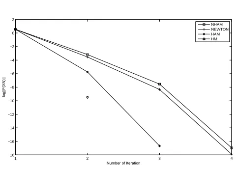
Table 1: Numerical results for Example 4.1 withx(0)= 1
Method NI ||F(x(m))|| CPU time result
NHAM 4 4.335133e−008 3.333667e+ 000 Convergent
Newton 4 1.691234e−008 7.639678e−002 Convergent
HAM 3 5.775537e−008 2.129251e−001 Convergent
HM − 7.457211e−005 4.041735e−001 Convergent
1 2 3 4
−18 −16 −14 −12 −10 −8 −6 −4 −2 0 2
Number of Iteration
log||F(XN)||
NHAM NEWTON HAM HM
Figure 1: The graph of ln(||F(X)||) for Example 4.1 withx(0)= 1
and Newton-HAM (NHAM) are reported. We utilize MATLAB 8. In Tables and Figures, the number of iterations (NI), the Euclidean norm of residual of government equation and CPU time, are presented.
Example 4.1. Consider the following equation:
f(x) =xex−1 = 0, (26)
The function f has at least one zero between 0 and 1. For x(0) = 1, the numerical results are shown in Table 1. For this initial point all methods are convergent, but the Newton method is apparently faster than other methods. Forx(0)= 10, the numerical results are shown in Table 2.
Table 2: Numerical results for Example 4.1 withx(0)= 10
Method NI ||F(x(m))|| CPU time result
NHAM 6 2.160101e−010 3.148814e+ 000 Convergent
Newton 16 5.107026e−014 2.622956e−001 Convergent
HAM 31 3.594237e−008 2.876829e+ 000 Convergent
HM − 5.790573e+ 003 4.081270e−001 Divergent
0 5 10 15 20 25 30 35
−35 −30 −25 −20 −15 −10 −5 0 5 10 15
Number of Iteration
log||F(XN)||
NHAM NEWTON HAM HM
Figure 2: The graph ofln(||F(X)||) for Example 4.1 withx(0)= 10
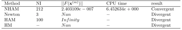
Table 3: Numerical results for Example 4.1 withx(0)=−400
Method NI ||F(x(m))|| CPU time result
NHAM 212 2.403109e−007 6.452634e+ 000 Convergent
Newton 3 N an − Divergent
HAM 100 Inf inity − Divergent
0 50 100 150 200 250 −100
−50 0 50 100 150 200 250
Number of Iteration
log||F(XN)||
NHAM NEWTON HM
Figure 3: The graph ofln(||F(X)||) for Example 4.1 withx(0)=−400
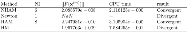
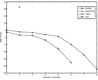
Table 4: Numerical results for Example 4.2
Method NI ||F(x(m))|| CPU time result
NHAM 6 2.085579e−008 2.116125e+ 000 Convergent
Newton 1 N aN − Divergent
HAM 8 2.247981e−010 3.105904e+ 000 Convergent
HM − 1.967763e+ 009 7.584255e−001 Divergent
Example 4.2. Consider following equations:
f1(x, y, z, d) =xyz+d−31 = 0,
f2(x, y, z, d) =x+y+z+d−11 = 0,
f3(x, y, z, d) = 2x+ 3y+ 4z+d−35 = 0,
f4(x, y, z, d) =x+z−y+d−1 = 0,
(27)
whereF =[f1f2f3f4
]T
.
We know ˆX1 = (2,3,5,1) and ˆX2 = (295,1110,5,−109) are two solutions of
F(X) = 0. ForX(0)= (1,1,1,1),numerical results are shown in Table 4.
Newton Method is divergent becausedet(DF(X(0))) = 0. But HAM and NHAM methods converge, and NHAM is faster than HAM.
1 2 3 4 5 6 7 8 −25
−20 −15 −10 −5 0 5 10 15 20 25
Number of Iteration
log||F(XN)||
NHAM NEWTON HAM HM
Figure 4: The graph ofln(||F(X)||) for Example 4.2
Table 5: Numerical results for Example 4.3
Method NI ||F(x(m))|| CPU time result
NHAM 8 6.567317e−010 8.196840e+ 001 Convergent
Newton 101 5.030214e+ 003 6.042236e+ 000 Divergent
HAM 18 5.830347e−008 3.106638e+ 003 Convergent
HM − 5.242329e+ 002 2.483993e+ 000 Divergent
f1(x1, x2,· · · , xn) = (3−12x1)x1−2x2+ 1 = 0,
fi(x1, x2,· · ·, xn) = (3−12xi)xi−xi−1−2xi+1+ 1 = 0, 1< i < n ,
fn(x1, x2,· · ·, xn) = (3−21xn)xn−2xn−1+ 1 = 0,
(28) that F=[f1f2· · ·fn
]T
.
Forn= 50 andX(0) = (100,100,· · ·,100), numerical results are shown in Table 5.
In this example HAM and NHAM are convergent to the exact solution ˆ
X = (1, ...,1), but Newton method is divergent. Also NHAM is faster than
HAM. Results are shown in Figure 5.
Example 4.4. Consider the following equations:
fk(x1, x2,· · ·, xn) = 10000xkxk+1−1 = 0, mod(k,2) = 1,
fk(x1, x2,· · ·, xn) =exp(−xk−1) +exp(−xk)−1.0001 = 0, mod(k,2) = 0,
0 10 20 30 40 50 60 70 80 90 100 110 120 −25
−20 −15 −10 −5 0 5 10 15 20
Number of Iteration
log||F(XN)||
NHAM NEWTON HAM HM
Figure 5: The graph ofln(||F(X)||) for Example 4.3
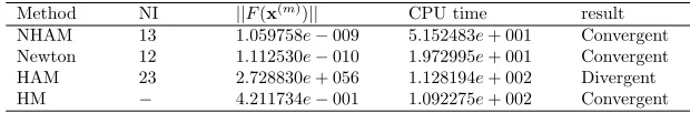
Table 6: Numerical results for Example 4.4
Method NI ||F(x(m))|| CPU time result
NHAM 13 1.059758e−009 5.152483e+ 001 Convergent
Newton 12 1.112530e−010 1.972995e+ 001 Convergent
HAM 23 2.728830e+ 056 1.128194e+ 002 Divergent
HM − 4.211734e−001 1.092275e+ 002 Convergent
that F=[f1f2· · ·fn
]T
.
For n = 100 and X(0) = (1,0,1,0,1,0,1,· · ·,0), numerical results are shown in Table 6. In this example Newton method, NHAM and HM are convergent, but HAM is divergent. Results are shown in Figure 6.
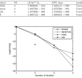
Example 4.5. Consider the following equations:
f1(x1, x2) =exp(x1) +x1x2−1 = 0,
f2(x1, x2) =sin(x1x2) +x1+x2−1 = 0,
(30)
that F=[f1f2· · ·fn
]T
.
1 2 3 4 5 6 7 8 9 10 11 12 13 14 15 16 17 18 19 20 21 22 23 24 25 −40
−20 0 20 40 60 80 100 120 140
Number of Iteration
log||F(XN)||
NHAM NEWTON HAM HM
Figure 6: The graph ofln(||F(X)||) for Example 4.4
Table 7: Numerical results for Example 4.5
Method NI ||F(x(m))|| CPU time result
NHAM 4 1.993082e−010 1.848117e+ 000 Convergent
Newton 4 1.405720e−012 2.472726e−001 Convergent
HAM 4 1.187309e−008 1.719704e+ 000 Convergent
HM − 5.368713e−006 1.380355e+ 000 Convergent
1 2 3 4
−30 −25 −20 −15 −10 −5 0
Number of Iteration
log||F(XN)||
NHAM NEWTON HAM HM
5 Conclusion
In this paper, Newton-HAM (NHAM) applying control parameterhare pro-posed for solving systems of nonlinear equations. The results for all examples are convergent and also NHAM is faster than Homotopy method. The re-sults demonstrate that by choosing a suitableh, HAM and NHAM methods are convergent. The numerical results show in general that the proposed method is effective and efficient and provides highly accurate results in a less number of iterations as compared by other methods. The main advantage of NHAM is the relative freedom of choosing initial guess. The appropriate proof convergence of NHAM can be continuation of the present work.
Acknowledgments
The authors would like to thank the anonymous referees for valuable com-ments and also express appreciation for their constructive suggestions.
References
1. Abbasbandy, S. Improving Newton-Raphson method for nonlinear equa-tions bymodifiedAdomian decompositionmethod, Applied Mathematics and Computation, 145 (2-3) (2003) 887-893.
2. Abbasbandy, S. and Jalili, M. Determination of optimal convergence-control parameter value in homotopy analysis method, Numerical Algo-rithms 64 (4) (2013) 593-605.
3. Abbasbandy, S., Tan, Y. and Liao, S.J.Newton-homotopy analysis method for nonlinear equations, Appl. Math. Comput. 188 (2007) 1794-1800.
4. Awawdeh, F. On new iterative method for solving systems of nonlinear equations, Numerical Algorithms, 54 (3) (2010) 395-409.
5. Babolian, E. and Jalili, M.Application of the Homotopy−Pad´etechnique in the prediction of optimal convergence-control paramete,Computational and Applied Mathematics, article in press. DOI:10.1007/s40314-014-0123-1, (2014).
6. Faires, J. and Burden, R.Numerical methods, Brooks Cole 3 edition, 2002.
8. Fang, L. and He, G.An efficient Newton-type method with fifth-order con-vergence for Solving Nonlinear Equations, Comput. App. Math., 27(3) (2008) 269-274.
9. Izadian, J., Mohammadzade Attar, M. and Jalili, M. Numerical solution of deformation equations in Homotopy analysis method, Applied Mathe-matical Sciences, 6(8) (2012) 357-367.
10. Liao, S. On the homotopy analysis method for nonlinear problems, Ap-plied Mathematics and Computation 147 (2004) 499-513.
11. Liao, S.Notes on the homotopy analysis method: Some definitions and theorems, Commun. Nonlinear Sci. Numer. Simulat., 14 (2009) 983-997.
12. Liao, S. The proposed Homotopy analysis technique for the solution of nonlinear problems,PhD thesis, Shanghai Jiao Tong University, 1992.
13. Liao, S. and Tan, Y. A general approach to obtain series solutions of nonlinear differential equations, Stud. Appl. Math 119 (2007) 297-354.
14. Liao, S. Beyond perturbation (Introduction to the homotopy analysis method), CHAPMAN and HALL , 2004.
15. Ku, C.Y., Yeih, W. and Liu, C.S. Solving nonlinear algebraic equations by a scalar Newton-homotopy continuation method, International Journal of Nonlinear Sciences and Numerical Simulation, 11(6) (2010) 435-450.
16. Stoer, J. and Bulrish, R. Introduction to numerical analysis, Springer, 1991.
HAM و ﻦﺗﻮﯿﻧ شور زا هدﺎﻔﺘﺳا ﺎﺑ ﯽﻄﺧ ﺮﯿﻏ تﻻدﺎﻌﻣ هﺎﮕﺘﺳد ﻞﺣ یاﺮﺑ ﺪﯾﺪﺟ شور ﮏﯾ
۲ﯽﻠﯿﻠﺟ ﻢﯾﺮﻣ و ،۱ﯽﻤﺸﯾﺮﺑا ﺎﺿﺮﻣﻼﻏ ،۱نﺎﯾدﺰﯾا لﻼﺟ
ﯽﺿﺎﯾر هوﺮﮔ ،مﻮﻠﻋ هﺪﮑﺸﻧاد ،ﺪﻬﺸﻣ ﺪﺣاو ،ﯽﻣﻼﺳ دازآ هﺎﮕﺸﻧاد۱ ﯽﺿﺎﯾر هوﺮﮔ ،مﻮﻠﻋ هﺪﮑﺸﻧاد ،رﻮﺑﺎﺸﯿﻧ ﺪﺣاو ،ﯽﻣﻼﺳ دازآ هﺎﮕﺸﻧاد۲
: هﺪﯿﮑﭼ
ﯽﭘﻮﺗﻮﻤﻫ ﺰﯿﻟﺎﻧآ شور و ﻦﺗﻮﯿﻧ شور زا هدﺎﻔﺘﺳا ﺎﺑ ﯽﻄﺧ ﺮﯿﻏ تﻻدﺎﻌﻣ هﺎﮕﺘﺳد ﻞﺣ یاﺮﺑ ﺪﯾﺪﺟ شور ﮏﯾ ﯽﯾاﺮﮕﻤﻫ مود ﻪﺟرد ﺖﻋﺮﺳ ندروآ ﺖﺳﺪﺑ و HAM ﯽﯾاﺮﮕﻤﻫ خﺮﻧ ﺖﻋﺮﺳ ﺶﯾاﺰﻓا .دﻮﺷ ﯽﻣ ﻪﺋارا (HAM) شور ﺎﺑ ﻪﺴﯾﺎﻘﻣ رد ار یدﺎﻬﻨﺸﯿﭘ شور دﺮﮑﻠﻤﻋ و ﯽﯾارﺎﮐ یدﺪﻋ ﺞﯾﺎﺘﻧ .ﺖﺳا شور ﻦﯾا ﯽﻠﺻا فاﺪﻫا ﯽﻠﮐ سﺪﺣ بﺎﺨﺘﻧا رد یرﺎﯿﺴﺑ یدازآ شور ﻦﯾا رد ﻪﮐ ،ﺪﻫد ﯽﻣ نﺎﺸﻧ HAM و ﻦﺗﻮﯿﻧ شور ،ﯽﻟﻮﻤﻌﻣ ﯽﭘﻮﺗﻮﻤﻫ .ﻢﯾراد ﻪﯿﻟوا شور ؛ﯽﯾاﺮﮕﻤﻫ لﺮﺘﻨﮐ ﺮﺘﻣارﺎﭘ ؛ﺮﻔﺻ ﻪﺒﺗﺮﻣ ﯽﺴﯾدﺮﮔد تﻻدﺎﻌﻣ ؛ﯽﭘﻮﺗﻮﻤﻫ ﺰﯿﻟﺎﻧآ شور : یﺪﯿﻠﮐ تﺎﻤﻠﮐ