Image Vectorization using Line Extraction and Filtering

Image Vectorization using Line Extraction and Filtering

Rajeev Bedi

Assistant Professor

BCET, Gurdaspur, Punjab Technical University, Jalandhar

Nisha Sharma

M.Tech. (Computer Science & Engineering) BCET, Gurdaspur, Punjab Technical University, Jalandhar

Abstract – The raster-vector conversion of remote sensing image is a very important task in the extraction and updating of linear objects in cartographic processes. In this paper we compare vectorization method and filtering method for the line extraction. Vectorization is based on constrained Delaunay triangulation, for line extraction. The constraints are provided by a preprocessing step insuring that these edges belong to line structures in the original image. The vectorization is performed using CDT and resulting triangles are grouped into polygons that make up the vector image. We use filter traces for a single road until a stopping criterion is satisfied. In this, approach, we use EKF with a special particle filter (PF) in order to regain the trace of the road beyond obstacles, as well as to find and follow different road branches after reaching to a road junction. In this paper, we have clearly discuss the advantages and disadvantages of both the algorithms over one another.

Keywords -Object recognition, Vectorization, CDT, skeletonization

I. I

The raster-vector conversion of remote sensing image is a very important task for extract and updating linear cartographic objects in cartographic processes. However, many troubles appear in the automatic solving of this problem. Normally segmentation and vectorization geometric techniques are used, as well as processes, models and patterns characteristics of the low, mid and high level of knowledge. On the other hand the variability in the geometrical structure and properties of the linear structure is so high that a manual process in order to improve automatic results is often needed. Thus more processing is needed to gather edges that belong to the same object. Many researched explored the possibilities of using the triangulation as a first step in performing image segmentation. This method involves thinning, line segment approximation, and geometric transformation. The skeleton line, obtained after the line segment approximation process, includes shape distortion caused by thinning. In the geometric transformation process, the line segments are shifted for minimizing the value defined in the neighbor of each corner, junction, and so on, by the smoothness and the difference between line segments and skeleton of an original image. The proposed method reduces various kinds of distortions, compared with other methods. Other important method focused on skeleton extraction. However

triangulation. Applying these filters eliminates the edges resulting from the triangulation that aren’t, thus creating polygons by adjacent triangles fusion. This process converts the original raster images into vector representation, which is a commonly used technique in graphics recognition problems as it puts the original image into a vector form that is more suitable for further analysis. Road is one of the important man-made objects whose information is important in cartography, urban planning, traffic management, and industrial development. Depending on whether a human operator interacts with the process or not, road extraction methods are categorized into automatic and semiautomatic methods. Different approaches have been proposed in literature to address the issue of automatic road extraction. One important class of road-tracking algorithms is based on probabilistic modeling of associated data and Bayesian estimation techniques. In these methods, statistical models are used to represent characteristics of the road features. In general, these approaches consist of two stages: prediction stage and update stage. The method based on the extended Kalman filter (EKF) is one of the methods in this class, which was first proposed for road map extraction in and then was further developed. Particle filters (PFs) are used for nonlinear filtering. Algorithms based on PF have been utilized to trace a single road path initiated by a given seed at the beginning of the road.

II. G

A

Copyright © 2012 IJECCE, All right reserved The main algorithm is preceded by a treatment that

provides points that are judged to belong to lines and will be introduced to constraints to the Delauny triangulation.

III. P

-P

A. Correlation

Correlation is a statistical measure of the association between variables. It summarizes the direction and closeness of linear relations between two variables. Correlation coefficients can range from -1 to +1. The value of -1 represents a perfect negative correlation while a value of +1 represents a perfect positive correlation. A value of 0 represents a lack of correlation.

The correlation coefficient is defined as:

where: p: current pixel r: reference pixel

Fig.2.1 The original image

Fig.2.2 Correlation distance image

Fig.2.3 High correlation

The correlation distance image (Fig 2.2) is scanned. To each pixel having a coefficient higher than a threshold t is assigned the gray level of the reference pixel. In the case where the current pixel has a low correlation coefficient, its spectral value is examined. If it has the same gray level as the reference pixel, the point is deleted. Thus the pixels that are highly correlated with the reference are emphasized (Figure 2). Then the pseudo codes of Computation of the high correlation image are as follows:

Fig.3.2 Extended neighborhood

The next step consists in applying a line detection method that is based on constrained gradient. The algorithm that has been described in relies on the fact that gradient vectors located in opposite sides of a line are pointing towards or against each other, according to the brightness of the line. The presence of a line can thus be detected by the calculation of the scalar product between opposite gradient vectors around a pixel.

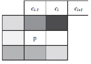
First, a gradient filter is applied to the image. Then, for a given pixel p, the symmetrical neighbors with respect to p in the immediate 8-vicinity, are arranged in pairs (ak. bk) as illustrated in Fig (Fig 4). The pair providing the higher (in absolute value) scalar product, noted (am. bm), gives the direction of the line. Afterwards, the further neighborhood is investigated while the scalar product is increasing. In this step, three other pairs are considered as illustrated in (Fig 3.2). The direction of the line is perpendicular to the pair giving the higher scalar product. To improve the line following, a non maximum deletion algorithm is applied. At each pixel the scalar product value is compared to the two adjacent pixels in the direction perpendicular to the line. If it is not maximum, the point is deleted, otherwise it is stored in a raster max Grad(i,j). The next step consists in line following. A line begins at a point of max Grad (i, j) that is larger than a threshold ts. Then, the algorithm moves to the maximum point in the 8 neighborhood if it is larger than a threshold tc. A line starts following the direction of this move and considering the max of the three next pixels ci-1, ci and ci+1(Fig 4).

A backward line is then followed using the opposite of the initial direction used in the first move. The result image still has areas that contain many scattered pixels. To remediate to this problem, a non-linear form deletion method is used. In fact, for a given pixel, if the immediate neighborhood contains a majority of white pixels, then it is not likely that it belongs to a line and is thus deleted. The result of this process is demonstrated in Fig 5.

Fig.5. Set of points resulting from the line following

IV. V

A. CDT

A triangulation of a set S of points on the plane presents a partition of an area, surrounded by a convex hull. Triangles are composed by vertices, given as an input. But if the triangles fulfill additional condition of an empty circumcircle, they present a Delaunay triangulation (DT).A triangulation T is a Delaunay triangulation of S if for each edge e of T there exists a circle C with the following properties: 1) the endpoints of edge e are on the boundary of C, and 2) no other vertex of S is in the interior of C. The Fig 7 shows an example of DT.

Copyright © 2012 IJECCE, All right reserved the following properties: the pre-specified edges are

included in the triangulation, and it is as close as possible to the Delaunay triangulation.

Let G be a straight-line planar graph. A triangulation T is a constrained Delaunay triangulation (CDT) of G if each edge of G is an edge of T and for each remaining edge e of T there exists a circle C with the following properties: 1) The endpoints of edge e are on the boundary of C, and 2) if any vertex v of G is in the interior of C then it cannot be ―seen‖ from at least one of the endpoints of e (i.e., if you draw the line segments from v to each endpoint of e then at least one of the line segments crosses an edge of G).

Fig.7. (a): A planar straight-line graph G(S,Ec). (b): Conventional Delaunay triangulation of the point set S. (c): Illustration of the modified circle criterion for constrained Delaunay triangulation

The presence of constraints in the CDT is ensured through local modifications where Delaunay edges are removed or flipped. CDTs solve the problem of enforcing boundary conformity—ensuring that triangulation edges cover the boundaries (both interior and exterior) of the domain being modeled. The image vectorization starts with Canny edge detection (see Fig 8) followed by a constrained Delaunay triangulation (CDT) where the lines resulting from the preprocessing stage are used as constraints for Delaunay triangulation.

Fig.8. Canny edge detection

Fig.9. Result of constrained Delaunay triangulation

B. Triangulation Edges Filtering

The generated triangle edges are then filtered. The constraints are kept while the other edges are filtered out according to a pre-specified set of rules. We use a well-known set of criteria for perceptual organization employed in human vision such as proximity, closure and contour completion. The proximity principle: elements tend to be perceived as aggregated into groups if they are near each other. Thus, edges are removed using a threshold filtering (Fig 10). The closure principle: elements tend to be grouped together if they are parts of a closed figure. In this case, the edges bounded by the same constraints are deleted (Fig 11). The contour completion rule states that between different contour edges, only the shortest edges are kept (Fig 12).

Fig.10. The dashed edge is not the shortest edge and hence should be deleted as it does not support proximity

Fig.11. The dashed edges are removed as they are bound by the same contour

After the edge filtering the image is segmented into a set of polygons. The result is a segmented image that is represented as a set of spectrally attributed polygonal patches: a vector image.

C. ROAD-TRACKING ALGORITHM

The road-tracking algorithm consists of two main modules: the EKF moduleand the PF module. These two modules alternately hand over the control of the process to each other, as explained in the following two sections. Fig. 6 shows the overall procedure of the road-tracking algorithm.

A. EKF Module

This module is initialized with a seed point given at the beginning of the road-tracking process. The starting point should include coordinates of the road center, road direction, and a coarse estimation of the road width at that point. The road center coordinates and the road direction are considered as the initial state of the system, namely, x1 (the fourth element of x1 is assumed to be zero). This starting point is also used to initialize the profile cluster (as mentioned in Section IV-A3).

The EKF module starts tracing the road using the initial state and the initial profile cluster. While progressing along the road path, the profile clusters are updated, and new appropriate clusters are added as road intensities and/or widths change. When the EKF module faces a severe obstacle on the road path or arrives at a road junction, the update profile cluster procedure cannot successfully create new profile clusters. This is due to the fact that the profiles extracted at road junctions or obstacles cannot pass validation tests or survive the authentication process after a pre-assigned number of steps since their creation. Therefore, the moving average of the profile error will increase and exceed a predefined threshold. This threshold determines where the EKF module should stop. This threshold can affect the overall outcome of the road detection algorithm. If it is set to a very low value, the EKF module will stop too often at each small obstacle or noise on the road path. On the other hand, a very high

and passes the control to the PF module. To initialize the PF module, the EKF module transfers the information about its last successful step of the present road segment onto the PF module.

B. PF Module

The PF module starts its work with a single road branch by using the last successful state estimate of the EKF module as its initial state x1. This module produces N particles from x1 and proceeds with the PF algorithm based on (14)–(17). The only major difference between the PF module and a regular PF algorithm is that, at step k, the PF module allows the existence of more than one final estimate of xk, with each associated with a potential road branch.

Copyright © 2012 IJECCE, All right reserved distance di,j = min{di,m}. The weight of the ith particle,

namely, wi, is calculated by using the likelihood function.

where D = 3 is the dimension of the measurement vector. previous is the weight of the ith particle of branch (b), in the (k − 1)th step.

Particles assigned to measurement m will be considered as particles of the new child branch branch (b).child (m), and each particle’s weight is acquired as described earlier. If there are less than N particles associated with branch (b).child (m), they will be resampling to N according to the re-sampling procedure described in Algorithm 2.

The aforementioned procedure will occur for every branch at the kth step. At the end, children of all branches will be accumulated to establish branches of the (k + 1)th step. Before going to the next step, a clustering algorithm is done on the new branches to merge the similar ones into a single branch. The clustering method is an agglomerative hierarchical clustering similar to the clustering method used for merging measurement data. The merging of branches will reduce transfer of redundant data to the next step and decrease the unnecessary processing load.

A validation test is performed at each step of the process on each branch. When the moving average prototype error of branch (b) increases beyond a predefined threshold (TBr), that branch is considered as spurious branch and is eliminated. In this case, the error of a branch is estimated based on two gray level profiles at each step of the processing of that branch: the between-edges profile and the along-the-road profile. The first profile is the portion of the previously mentioned crossroad profile which lies between the estimated edges of the road. The second profile is a profile extracted on the road center and along the road angle. Since a road has relatively homogenous intensity in comparison with the off-road areas, these two orthogonal profiles have low variations in their gray-level values if we are correctly located on the road axis with a right orientation. Therefore, the gray-level variations in these two profiles provide a means to identify a real road branch from a spurious one in the PF algorithm. The gray-level variation is measured by calculating the average forward difference on each of the profiles. This criterion is computed for each branch of the algorithm at each time step. If, for branch (b), the time average of the criterion exceeds TBr, then this branch will be eliminated. We have experimentally found that the proper value for TBr is 15 in

a 256-gray-level image. Using much higher values for this parameter, i.e., 30 or more, causes the PF module to maintain too many unnecessary hypothetical branches, many of which might be related to off-road errors and not representing real road branches. This causes the PF module to become very slow since it has to run an instance of PF for each branch. On the other hand, by decreasing TBr, i.e., to five or less, we might decrease the chances of tracking some of the real road branches originating from a road junction beyond an obstacle. As a result, this threshold has an important role in the overall performance of the road network detection. The PF module will stop after S number of steps. The value of S must be large enough to let the PF module to pass over regular-sized obstacles and junctions. Therefore, the choice for the value of S depends on a rough estimation of the size of the regular road junctions and blocking, as well as the resolution of the satellite image. For example, if we assume that the largest junction is about 100 m long and the spatial resolution of the image is 5.8 m, we then need to set S to 100/5.8 = 17.24 or 18 steps. When the PF module precedes S number of steps, it is likely to find road branches that are beyond the road junctions or to find the continuation of a road beyond a blocking that is as big as 100 m. After S number of steps, the PF module stops and classifies the final branches into as many distinctive road branches as it can distinguish. The estimated state associated with each branch can be considered as a new seed point that can, in turn, launch the EKF module to trace a new road segment. If the PF module cannot find any valid road branches after S steps, it will announce that the road is a dead-end road.

the same time. Therefore, it can find and track road branches that are originated and dispersed from a road junction. Furthermore, in the case of a road obstacle, this module can proceed with different directions until it finds the right road path(s) at the other side of the obstacle. If, however, after some pre-assigned steps, the PF module is not able to find any valid road branches (when the moving average error of all branches exceeds the threshold), then the road is considered to be terminated.

V. R

C

A Skeletonization

Skeletonization is a transformation of a component of a digital image into a subset of the original component. It is a global space domain technique for shape representation that has been studied extensively since skeletons have attractive properties which make them suitable for structural pattern recognition. The skeleton typically emphasizes the geometric properties and topological shape, such as connectivity, topology, length, direction, and width. There are two well-known paradigms for skeletonization methods: The first is iterative thinning of the original image until no pixel can be removed without altering the topological and morphological properties of the shape. The second definition used for a skeleton is that of the ridge lines formed by the centers of all maximal disks included in the original shape, connected to preserve connectivity. This leads directly to the use of distance transforms or similar measures which can be computed in only two passes on the image.

Fig.13. A set of objects with skeletons superimposed.

The final step in our algorithm is to extract the skeleton of the obtained polygons. The skeleton represents the extracted lines.

Fig.14. (b) The extracted lines (skeletonization result)

B. Computational Cost

The Canny edge detection is a fast linear method. The computational time complexity of Canny algorithm is a linear function of the number of pixels in the image. A divide and conquer algorithm for triangulations in two dimensions was proposed in and improved by Guibas and Stolfi and later by Dwyer. The merge operation can be done in time O (n), so the total running time is O (n log n) in function of contour points which is equal to the number of pixels in the detected edges. This can be improved using sub-sampling.

C Road Extraction Results

We have applied our proposed technique to a real satellite image of Kish Island in Iran. The satellite image is a panchromatic image of the Indian Remote Sensing (IRS) satellite with 5.8-m spatial resolution. We have also processed another satellite image with a higher resolution. This image is a satellite image of IKONOS with 0.8-m resolution.

Copyright © 2012 IJECCE, All right reserved different. The EKF module should properly find and

estimate the coordinates of the road median, while the PF module is only utilized in critical situations, i.e., when the EKF module stops due to road obstacles or road junctions. The important parameters used in our algorithm are specified in Table III. The step size dt determines the distance, in pixels, between the process point of the algorithm at step k and step k − 1. For larger dt, progress of the EKF and PF modules will be faster on the image; however, the resolution of the resulting road center points will be coarser. The system error co-variances matrix Qk is a measure of how our road model matches. If the roads in the image are changing direction rapidly, we have to set high values for the elements of Qk. The measurement error covariance matrix Rk models the behavior of the error resulted from our measurements from the image. The values of Qk and Rk in Table III are better to be adapted based on the type and content of the satellite image. However, the output is not very sensitive to these values. We have used the same values for both sample images. The parameters Δ, ϕ, and dϕ are discussed in Section IV-A1. Among the parameters in the table, the last three thresholds are more important in changing the completeness and correctness of the results. Some of these thresholds partly depend on the image and road properties, e.g., the edge detection threshold TEg. The aforementioned parameter can be tuned more precisely during a training stage prior to the start

Fig.15. Different stages of the overall road-tracking algorithm on an IRS image. (a) First road segment extracted by the EKF module. (b) Particles of the PF module. (c) Road branches

extracted by the PF module. (d) Second road segment extracted by the EKF module. (e) Road branches extracted by the PF module. (f) Third road segment extracted by the EKF module. (g) Final result of the road extraction algorithm. (h) Road reference points extracted manually of the main road tracing algorithm. This means that, before processing a satellite image, we can ask the operator to identify some instances of road centers and their directions. Then, a training algorithm can use the road profiles, obtained from the provided seed points, as examples used to find an appropriate value for the edge threshold. The other two parameters, namely, TBr and TMrg, and their relevance to the outcome of the algorithm are discussed.

Fig. 15(a) shows the extraction of the first road segment by the EKF module. The EKF module has traced the road until it encounters the junction. At this point, the EKF module hands over the process to the PF module, which distributes the particles in the way shown in Fig. 15(b). The seed points of the final extracted road branches, following the process of the PF module, are marked with white pixels in Fig. 15(c). The first seed point, i.e., the one closer to the bottom of the image,

Fig.6. Final results of the road-tracking algorithm on an IKONOS image

Fig.7. Road reference points extracted manually.

15(d). This instance of the EKF module stops after facing another junction in the bottom of the image and, again, hands over the process to the PF module. The distribution of road branch particles at the end of this instance of the PF module is shown in Fig. 15. Fig. 15(f) shows the outcome of this instance of the PF module followed by another instance of the EKF module which traces the third road segment. The algorithm continues in the same manner until it finds all the connected road segments. The final result is shown in Fig. 15(g). In Fig. 15(h), you can see the reference points of the road network extracted manually by an operator. Fig. 16 shows the final result of the road-tracing algorithm on the IKONOS image. The reference road network is shown in Fig. 17.

Black pixels on the image represent the output results of both EKF and PF modules. The line segments show road branch axes traced by the EKF module, while the numerous distributed black points at road intersections are the center points of branches resulted from the PF module. In Fig. 16, the algorithm starts from an initial point at the top right corner of the image and runs the first instance of the EKF module to track the road branch on the left. Altogether, the EKF module has recognized 18 junctions and obstacles on this image. It has missed six junctions, most of which do not comply with the implicit junction model inherent in our method. The crossroad profiles right at the place of the missing junctions look like a regular road profile without any road branches connected to the side of the road. This is due to the fact that, at those intersections, there is a line between the main road and the connecting branch which looks like a road edge and therefore makes the junction less similar to a junction model. At all 18 instances of junction/obstacle recognition, the control was passed to the PF module. If there was a road intersection, the PF module has always found all road branches originated from that intersection. On the other hand, if there was a dead-end road, the PF module has correctly decided to end the road. These dead-end points are indicated in Fig. 8 by black squares. The PF module decides a dead end following the rejection of all hypothetical branches through the branch validation criterion. For evaluating the results, we have used an operator generated image as our reference for a road network axis. The results are evaluated using important evaluation metrics called correctness and completeness. Correctness shows how much the extracted road pieces correspond to a real road. On the other hand, completeness is a measure of how much the extracted network is completed. In order to find the correctness measure of our results, branch segments extracted by the EKF module were used. The center points resulted from the PF module on hypothetical branches were discarded due to the fact that they do not show a clear road axis position. For both IRS and IKONOS images used in our experiments, the

that, in both experiments, there is only a single initial starting point that is fed to the algorithm by the operator.

6. CONCLUSION

In this paper our approach of automatic line is detection using image vectorization and filtering. The algorithm provides good results on both levels of completeness and exactness as indicated by the recall and precision values. A deficiency of the algorithm is the slow operation of the PF module. However, since the PF module executes only on road junctions and/or road obstacles, its slow operation does not affect the entire process of the road-tracking algorithm. It should also be noted that the proper setting of the parameters used in this algorithm affects the performance of the road extraction (as it is true for most automatic systems). Furthermore, performance of the algorithm on more complex urban areas is yet to be evaluated, which might necessitate some modifications in the way measurements are acquired.

R

[1] Prasad, L., Skourikhine, A. N., 2006. Vectorized image segmentation via trixel agglomeration. Pattern Recognition, 39(4), pp. 501-514.

[2] N. Skurikhin a, P. L. Volegov b. OBJECT-ORIENTED HIERARCHICAL IMAGE VECTORIZATION

[3] Sriram Swaminarayan, Dr. Lakshman Prasad, RaveGrid: Raster to Vector Graphics for Image Data, SVG Open 2007

[4] Wertheimer M., 1958. Principles of perceptual organization. In: Readings in Perception, Beardslee, D., Wertheimer, M., (Eds.), D. Van Nostrand, Princeton, NJ, pp. 115-135.

[5] Ching-Chien Chen , Craig A. Knoblock andCyrus Shahabi. Automatically Conflating Road Vector Data with Orthoimagery. GeoInformatica (2006) 10: 495–530

[6] J. Mena, ―State of the art on automatic road extraction for GIS update: A novel classification,‖ Pattern Recognit. Lett., vol. 24, no. 16, pp. 3037–3058, Dec. 2003.

[7] G. Vosselman and J. D. Knecht, ―Road tracing by profile matching and Kalman filtering,‖ in Proc. Workshop Autom. Extraction Man-Made Objects Aerial Space Images, Birkhaeuser, Germany, 1995, pp. 265–274.

[8] A. Baumgartner, S. Hinz, and C. Wiedemann, ―Efficient methods and interfaces for road tracking,‖ in Proc. Int. Arch. Photogramm. Remote Sens., 2002, vol. 34, pp. 28–31.

A

’

P

Rajeev Bedi

Assistant Professor

BCET, Gurdaspur, Punjab Technical University, Jalandhar

Nisha Sharma

M.Tech. (Computer Science & Engineering)