R E S E A R C H A R T I C L E
Open Access
Visualizing inconsistency in network
meta-analysis by independent path
decomposition
Ulrike Krahn
1,2, Harald Binder
2and Jochem König
2*Abstract
Background: In network meta-analysis, several alternative treatments can be compared by pooling the evidence of all randomised comparisons made in different studies. Incorporated indirect conclusions require a consistent network of treatment effects. An assessment of this assumption and of the influence of deviations is fundamental for the validity evaluation.
Methods: We show that network estimates for single pairwise treatment comparisons can be approximated by the evidence of a subnet that is decomposable into independent paths. Path-based estimates and the estimate of the residual evidence can be used with their contribution to the network estimate to set up a forest plot for the
consistency assessment. Using a network meta-analysis of twelve antidepressants and controlled perturbations in the real and constructed consistent data, we discuss the consistency assessment by the independent path
decomposition in contrast to an approach using a recently presented graphical tool, the net heat plot. In addition, we define influence functions that describe how changes in study effects are translated into network estimates.
Results: While the consistency assessment by the net heat plot comprises all network estimates, an independent path decomposition and visualisation in a forest plot is tailored to one specific treatment comparison. It allows for the recognition as to whether inconsistencies between different paths of evidence and outlier effects do affect the considered treatment comparison.
Conclusions: The approximation of the network estimate for a single comparison by the evidence of a subnet and the visualisation of the decomposition into independent paths provide the applicability of a graphical validation instrument that is known from classical meta-analysis.
Keywords: Network meta-analysis, Multiple treatments comparison meta-analysis, Mixed treatment comparison meta-analysis, Inconsistency, Influence diagnostics, Forest plot
Background
In medical practice, several treatments are frequently suit-able for a single indication, but often only two or three of them are directly compared in one study. Network meta-analysis is an approach that combines the informa-tion from all clinical trials on any of the treatments based on the assumption of consistent treatment effects and the inclusion of indirect comparisons (for an overview
*Correspondence: [email protected]
2Institute of Medical Biostatistics, Epidemiology and Informatics, University Medical Center Johannes Gutenberg University Mainz, Langenbeckstr. 1, 55101 Mainz, Germany
Full list of author information is available at the end of the article
see e.g. [1]). The evaluation of the consistency and the influence of possible deviations of this assumption on network estimates plays an important role in the vali-dation of results [2], especially as more complex models are fitted [3]. In classical meta-analysis, a forest plot of study effects and the pooled estimate offers the visual-isation of outlier effects and their contribution to the aggregated treatment effect [4]. In network meta-analysis, the homogeneity between studies of each pairwise treat-ment comparison can also be analysed using forest plots. However, to assess the consistency assumption in the net-work, study-based forest plots are not directly applicable,
since for different pairwise treatment comparisons vari-ous effects are expected [1]. Therefore, a generalised forest plot approach is needed.
Salanti et al. [5] graphically analysed consistency using a forest plot of the differences between direct and indi-rect evidence in single network loops. In a forest plot, estimates based on direct, indirect (obtained by back-calculation or node-splitting [6]), and combined evidence for one treatment comparison can be compared [1,2] without reflecting detailed sources of potential inconsis-tencies. Tools for regression diagnostics like the plot of posterior mean deviance of individual data points [6,7], the plot of leverage against the residual deviance for each data point [8], or the assessment of PRESS residuals and studentised residuals [9] allow for the singling out of indi-vidual studies or a set of studies that compared the same treatments whose direct evidence is badly fitted and may be responsible for heterogeneity or inconsistency. For an influence analysis of potentially inconsistent direct evi-dence, the contribution of direct evidence to network estimates has to be taken into account. Krahn et al. [10] proposed a matrix visualisation, called net heat plot, that highlights hot spots of inconsistency between specific direct evidence in the whole network and renders possible drivers transparent.
None of these approaches can offer all the analytical capacities available in a classical meta-analysis forest plot to a consistency assessment in a network meta-analysis: namely the composition of the network effect estimate based on direct evidence, the consistency between differ-ent evidence sources, outlier observations and the influ-ence on aggregated treatment effect estimates.
In the following, we show that a single network effect estimate (e.g. for the comparison between treatmentsA and B) can also be approximated by the evidence of a subnet that is decomposable into independent paths and can be visualised in a forest plot. For a consistency inves-tigation, it allows the visualisation of the contribution of each independent path as well as that of the residual evidence in combination with their corresponding treat-ment effect estimate. Due to the additional display of the network-based treatment effect, an influence assessment of deviating direct evidence is possible. We discuss this tool for consistency and influence assessment in contrast to the net heat plot [10] by using an evidence network of twelve antidepressants. We assess controlled perturba-tions in a constructed, consistent dataset of the example and subsequently in the real data.
This article is structured as follows: We start with the data example. In the Methods section, we discuss the influence of direct evidence in network meta-analysis and derive an influence function as well as the concept of a decomposable subnet approximation and its visualisa-tion. In the Results section, we apply our approach to the
data and compare it with net heat plot results. The paper concludes with a discussion of our findings.
Application
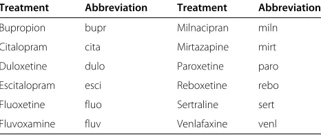
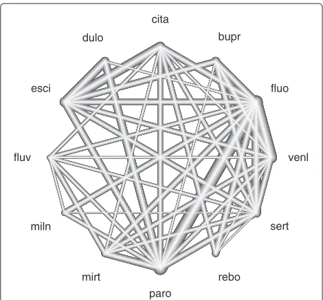
As a data example, we consider a network meta-analysis performed by Cipriani et al. [11] (for data availability see [11]). In this analysis, twelve antidepressants (see Table 1) are examined regarding response, defined as a reduction of at least 50% from the baseline of the depression rat-ing score after eight weeks. The odds ratio (OR) was used as effect measure. In total, 111 randomised trials are included in this network meta-analysis comprising 109 two-armed trials and two three-armed trials. Figure 1 shows the complexity of the network; the assessment of inconsistency and influence of perturbations pose a challenge.
Methods
In the following, we briefly present a fixed effects model for network meta-analysis that has already been explained in more detail by Krahn et al. [10] and in this context analyse how changes in study effects are translated into network estimates. We introduce a simplification of meta-analysis networks into decomposable subnets that allows the application of a forest plot for a single network-based treatment effect.
Fixed effects model in network meta-analysis
We consider a network meta-analysis forT+1 treatments A0,. . .,AT that are compared in a set of studies
build-ing a connected evidence network as for instance shown in Figure 1. Assuming consistency, all pairwise treatment effects in the network are uniquely determined by the T basic contrasts to a reference treatmentA0, which we denote by the vector θnet. Characterising each study by the investigated set of treatments (called design in the context of network meta-analysis [12,13]), it has been demonstrated that the generalised least squares estima-tion for a fixed effect model can be partiestima-tioned into two steps [10]: Firstly, the evidence is pooled for each designd (d = 1,. . .,D) to get an aggregated treatment effectθˆddir
Table 1 Twelve antidepressants examined in the network meta-analysis published by Cipriani et al. [11]
Treatment Abbreviation Treatment Abbreviation
Bupropion bupr Milnacipran miln
Citalopram cita Mirtazapine mirt
Duloxetine dulo Paroxetine paro
Escitalopram esci Reboxetine rebo
Fluoxetine fluo Sertraline sert
fluo bupr
cita
dulo
esci
fluv
miln
mirt
paro
rebo
sert venl
Figure 1Evidence network of the antidepressants example.The lines display the observed treatment comparisons. The thickness of a line is proportional to the inverse standard error of the directly estimated treatment effect, which is aggregated over all studies including the two respective treatments.
(e.g. an aggregated log(OR)) with covarianceVddir. (In the case thatdis a design of one or moreNd-armed studies,
ˆ θdir
d is a vector of length(Nd−1)andVddira matrix of size
(Nd−1)×(Nd−1); for a detailed explanation see [10]).
Secondly, the vector of all direct treatment effect estimates ˆ
θdir :=θˆdir
1 ,. . .,θˆDdir
and the known covariance matrix
V := Cov() = diagV1dir,. . .,VDdirare used to fit the model:
ˆ
θdir=Xθnet+. (1)
The design matrix X comprises one column for each
treatment A1,. . .,AT and one row for each design and
each comparison with a design-specific reference (i.e.d (Nd−1)rows). If included in a design, this design-specific
reference equalsA0. The entries ofXhave value 1 in the column corresponding to the treatment compared with the reference, -1 in the column corresponding to a design-specific reference whenever it is notA0, and 0 else. The vector of all error terms is assumed to be independent across designs and normally distributed with covariance matrixV.
The vector of basic contrastsθnetcan then be estimated by generalised least squares as
ˆ
θnet=Bθˆdir,B=XV−1X−1XV−1
with predicted effectsXθˆnet=Hθˆdir. Thereby, the matrix H = XBprojects the estimates based on direct evidence
to the network estimates and provides in each row the lin-ear coefficients for one network estimate. Thus, a network estimate of treatmentuversus treatmenttis composed as follows:
ˆ θnet
tu =Htu,.θˆdir=
D
d=1
htu,dθˆddir,
whereHtu,.denotes one row vector, andhtu,ddenotes one
entry (or in the case thatdis a design of one or moreNd
-armed studies, a transposed partial row vector of length (Nd−1)) ofH.
Influence of single studies or designs in network meta-analysis
In classical meta-analysis, a study with a highly deviating treatment effect estimate may have a strong influence on the aggregated effect estimate depending on its weighting in the estimation process. Using generalised least squares estimation, the weight is proportional to the inverse vari-ance of the treatment effect estimate.
In network meta-analysis, the weighting of a study in one network estimateθˆtunet depends not only on its cor-responding precision, but also on the network structure: Studysof designdwith covariance matrixVscontributes
in model (1) to the aggregated treatment effect estimate ˆ
θdir
d with weight Ws =
s∈SdV −1
s
−1
Vs−1, where Sd
denotes the set of all studies with design d. The direct treatment effect estimateθˆddirin turn drives a network esti-mateθˆtunetby the value of the corresponding elementhtu,d
of matrixH. So, the contribution of studysis given by
htu,s=htu,dWs.
If treatment effect estimateθˆddirof designdis inconsis-tent with the treatment effect estimates of the remaining network, the question arises as to how this influences a network estimateθˆtunet. Therefore, we define an influence function as the change in a network estimate when the direct treatment effect estimateθˆddiris shifted byδ. For a design of two-armed studies, this means ifθˆdir → ˆθdir+ δedwhereeddenotes the unit vector with 1 at positiond
and 0 elsewhere,
IFtu,d(δ;X,V):= ˆθtunet
ˆ θdir+δe
d
− ˆθnet
tu
ˆ θdir
=Htu,.θˆdir+δHtu,.ed−Htu,.θˆdir
=δhtu,d.
In the case of multi-armed designs, influence functions for each pairwise comparison can be defined similarly.
Net heat plot
effects and the aggregated treatment effect are, for exam-ple, visualised in a forest plot. For a similar analysis in network meta-analysis, a so-called net heat plot has been proposed [10]. In a matrix visualisation (see examples in the Results section), the contribution of the aggregated direct evidence of each design (in a column) to each net-work estimate (in a row) is shown by the area of gray squares. The greater the area of a square, the greater the contribution of the respective direct evidence to the network estimate in the row. In combination with this evi-dence flow, a heat matrix for assessing the inconsistency in the network (quantified by a generalized Cochran’sQ statistic) is shown: The colours on the diagonal repre-sent the inconsistency contribution, the summand of the Cochran’s Q statistic, of the corresponding design. The colours on the off-diagonal are associated with the change in inconsistency between direct and indirect evidence in a network estimate in the row after relaxing the consistency assumption for the effect of one design in the column. Blue colours indicate an increase and warm colours a decrease. In the case that the colour vector of a column is equal to the colour vector on the diagonal, the detachment of the respective design resolves the inconsistency in the whole network.
The detaching of single designs is similar to the node splitting technique of Dias et al. [8], but the net heat plot approach additionally tracks the influence of each design on the fit on all other designs and visualises the succes-sive detaching of each designs in one plot. In contrast, the approach to the consistency assessment presented in the following allows for the application of a forest plot for one specific treatment comparison.
Decomposable subnets
For the assessment of consistency and influence in one network-based comparison, we use a simplification of the network into a decomposable subnet. Firstly, we will describe our approach for networks formed only by two-armed studies and we will refer to the case of multi-two-armed studies in Section ‘Multi-armed designs’.
A treatment effect estimate between treatments tand u is most easily assessable if the underlying network is entirely composed of independent paths between the treatment nodes u andt (see also [14]). Two paths are defined as independent if they do not share any edges. Each path-based estimate can be formulated by the sum over the intermediate effect estimates. For example, the indirect estimate for treatment effectuversustvia treat-mentvcan be calculated byθˆtvdir + ˆθdir
vu [15]. Path based
estimates of independent paths are uncorrelated because they are based on independent evidence. The variance is obtained by summing up the direct estimate variances as described by Bucher et al. [15]. All path-based esti-mates are combined as a weighted sum with weights
proportional to their inverse variances. For assessing the consistency, we display this aggregation step in a for-est plot where each row represents a path-based effect estimate and each path is identified by its unique list of intermediate treatments.
If the given network is not decomposable as described above, we consider the set of all decomposable subnet-works and choose one with the most precise resulting effect estimate. Although challenging in general, it is often easy to find a well approximating decomposable subnet just by selecting all paths containing no or only one inter-mediate treatment. Note that in a network represented by a complete graph with direct effect estimates of constant precision, the best approximating decomposable subnet (i.e. with the most precise resulting effect estimate) is uniquely defined by the direct path and all two-step indi-rect paths [16]. The resulting estimate is identical to the network-based estimate.
Once an approximating decomposition is achieved, we denote the corresponding network estimate as θˆtuapprox. The residual evidence of the network can be defined as the pseudo effect estimate
ˆ θres
tu :=
ˆ θnet tu var ˆ θapprox tu
− ˆθapprox
tu var ˆ θnet tu
varθˆtuapprox−varθˆtunet ,
with precision
var−1
ˆ θres
tu
=var−1
ˆ θnet
tu
−var−1
ˆ θapprox
tu
(see analogously the back-calculation in [8]). Then, the network-based estimate is the weighted sum
ˆ θnet
tu =w
approx
tu θˆ
approx
tu +
1−wapproxtu θˆtures
with
wapproxtu := var ˆ θnet tu var ˆ θapprox tu .
This weight describes the proportion of evidence for the given effect that is contained in the subnetwork. In the following, we refer to it as approximating evidence pro-portion. Note that the variance of the difference between the network and the subnetwork-based estimate is
varθˆtuapprox− ˆθtunet=varθˆtuapprox−varθˆtunet,
which can be used to straightforwardly define aZstatistic to test for consistency between the approximation and the network-based estimate (by analogy with e.g. [16]).
Forest plot
and, at a higher level, how the subnet contributes to the whole network-based estimate (see examples in the Results section). The resulting overall Cochran‘sQ statis-tic has degrees of freedom (df ) equal to the number of independent paths. It is similar but not identical to the inconsistency Q [10]. It captures solely that aspects of inconsistency that have consequences for the uncertainty about the effect estimateθˆtunet. The weights in the forest plot can be interpreted as the proportion at which a per-turbation in any direct estimate contributing to that path is translated into a bias of the network estimate θˆtunet. If the weight of the residual evidence is small, no perturba-tion outside the subnet at any plausible scale is able to substantially affect the network estimate.
Iterated shortest path algorithm
The enumeration of all decomposable subnets may be too cumbersome. We therefore propose a simple algorithm that aims to find a good, but not always the best, approx-imating decomposable subnetwork. We therefore define the distance between two adjacent nodes as the variance of the corresponding direct effect estimate, and the length of a path is identical to the variance of the path-based effect estimate. The proposed algorithm is as follows:
1. Start selecting the shortest path between nodestand
uand eliminate all its edges [17].
2. Iterate until the nodestanduare no longer connected.
The set of all eventually selected paths make up the approximating sub-network and its independent path decomposition.
Multi-armed designs
Different strategies can be used for multi-armed designs: Firstly, they can be kept out of all paths of a subnetwork of independent paths. Secondly, one convenient treatment comparison for each multi-armed design, for example, the comparison between A and B for the multi-armed design ABC, can be allowed to potentially contribute in com-bination with all two-armed studies of design AB. This implicitly assumes that direct evidence for the relative effectθtu does not depend on the remaining treatments
investigated in the same study. A further strategy is to use at most one comparison (e.g. AB) of each multi-armed design separated from all two-armed studies (of design AB) and to build extra paths with these comparisons if possible. For the examples discussed in the following, we use the first strategy.
Construction of validation datasets
In the Results section, we illustrate the influence analysis and the decomposition of an evidence network into inde-pendent paths based on the antidepressants example. For
validating the analysis capabilities for the proposed path-based forest plot assessment in contrast to the net-heat plot approach, we use controlled perturbations, firstly in a constructed, consistent dataset and then in the real data. We constructed the consistent network of treatment effects based on the antidepressants example by setting the OR of all studies to one and retaining all standard errors. The corresponding net heat matrix is drawn in Figure 2a. Perturbations were effected by adding aδ = log(2)to selected log odds ratiosθˆddir.
Results
We demonstrate the influence analysis as well as the approach of the independent path decomposition and its visualisation by applying the methods to the antidepres-sants example. The analysis capability by the indepen-dent path decomposition is discussed in comparison to the net heat plot approach using controlled perturba-tions in the consistent validation dataset as well as in the real data. To produce the forest plots and the net heat plots, we used functions of the R packages meta [18] andnetmeta[19]. Software instructions and anR func-tion for the iterated shortest path algorithm are available on the website http://www.unimedizin-mainz.de/imbei/ biometrie/software.html.
Influence analysis
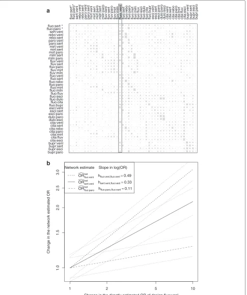
The contribution of all design-specific direct evidence to the network estimates in the antidepressants example is visualised in Figure 2a. The areas of the gray squares are determined by the elements of the projection matrixHof the underlying model (as well as in [10]). As seen from the column of design fluo:venl for example, the correspond-ing direct estimate represents a large source of evidence as it drives the network estimates for many treatment con-trasts. In particular, (as visualised by the area of the gray square in the diagonal element fluo:venl) the network esti-mate for fluo:venl is based on 49% direct evidence of 11 studies with inverse variance weights between 2.1% and 16.3%. The contribution of single studies to the network estimate is therefore beween 1% and 8%.
bupr:parobupr:esci bupr:sert bupr:venlcita:esci cita:fluv cita:mirt cita:paro cita:rebocita:sert cita:venl dulo:esci dulo:paro esci:paroesci:sert esci:venl fluo:buprfluo:cita fluo:dulo fluo:escifluo:fluv fluo:milnfluo:mirt fluo:paro fluo:rebofluo:sert fluo:venl fluv:milnfluv:mirt fluv:parofluv:sert fluv:venl miln:paromiln:sert mirt:paromirt:sert mirt:venl paro:sert paro:venlrebo:sert rebo:venlsert:venl fluo:paro *fluo:sert *
fluo:sert* fluo:paro* sert:venl rebo:venl rebo:sert paro:venl paro:sert mirt:venl mirt:sert mirt:paro miln:sert miln:paro fluv:venl fluv:sert fluv:paro fluv:mirt fluv:miln fluo:venl fluo:sert fluo:rebo fluo:paro fluo:mirt fluo:miln fluo:fluv fluo:esci fluo:dulo fluo:cita fluo:bupr esci:venl esci:sert esci:paro dulo:paro dulo:esci cita:venl cita:sert cita:rebo cita:paro cita:mirt cita:fluv cita:esci bupr:venl bupr:sert bupr:esci bupr:paro
Network estimate Slope in log(OR)
ORfluonet:venl h
fluo:venl,fluo:venl=0.49
ORsert:venl net
hsert:venl,fluo:venl=0.33
ORfluo:paro net
hfluo:paro,fluo:venl=0.11
1 2 5 10
1.0
1.5
2
.0
2.5
3.0
Change in the directly estimated OR of design fluo:venl
Change in the network estimated OR
a
b
2.00 [1.67;2.39] instead of 1.00 [0.84;1.2] shifts the network estimates for comparisons fluo:paro, sert:venl, fluo:venl from 1.00 [0.89;1.12], 1.00 [0.86;1.17], and 1.00 [0.88;1.13] to 1.08 [0.96;1.21], 1.26 [1.08;1.47], and 1.41 [1.24;1.59]. Such a deviation of the direct evidence of design fluo:venl from the assumption of consistency would bias the net-work estimates of comparisons sert:venl and fluo:venl to at 5% level significant treatment effects.
Approximation by independent path decomposition The network of antidepressants shown in Figure 1 is highly complex and interconnected. It has 42 edges
supported by direct evidence including two three-armed studies. But a lot of treatment comparison estimates in this network meta-analysis are dominated by direct and simple indirect evidence including only one intermediate treatment.
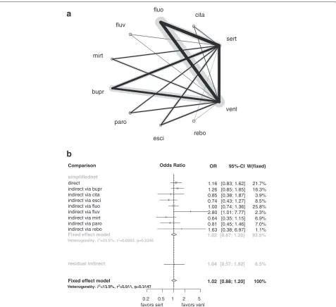
For example, the network estimate of comparison sert:venl is primarily based on direct evidence with 22% and on eight indirect comparisons including only one intermediate treatment (via bupr, cita, esci, fluo, fluv, mirt, paro, and rebo). This independent path decomposition is shown in Figure 3a and is the result of the iterative shortest path algorithm. The corresponding forest plot is displayed
bupr
cita
esci fluo
fluv
mirt
paro
rebo
sert
venl
Comparison
Fixed effect model
Heterogeneity: =13.9%, =0.011, p=0.3147 simplifiednet
residual indirect Fixed effect model
Heterogeneity: =23.5%, =0.0203, p=0.2345
direct indirect via bupr indirect via cita indirect via esci indirect via fluo indirect via fluv indirect via mirt indirect via paro indirect via rebo
Odds Ratio
0.2 0.5 1 2 5 favors sert favors venl
OR
1.02
1.02
1.04
1.16 1.26 0.85 0.74 1.00 2.80 0.64 0.81 1.63
95%-CI
[0.88; 1.20]
[0.87; 1.20]
[0.57; 1.92]
[0.83; 1.62] [0.85; 1.85] [0.38; 1.87] [0.43; 1.27] [0.74; 1.36] [1.01; 7.77] [0.35; 1.15] [0.45; 1.46] [0.38; 6.97]
W(fixed)
100%
93.5%
6.5%
21.7% 16.3% 3.9% 8.5% 25.8% 2.3% 6.9% 7.0% 1.1%
a
b
in Figure 3b. The approximation by the independent paths provides 93.5% of the whole network’s evidence regarding the estimation of the treatment comparison sert:venl.
This display shows fairly consistent independent path-based estimates with exception of the indirectly estimated treatment effect via fluv with OR 2.8 [1.01;7.77]. Since the contribution of this estimate is 2.3%, the network esti-mate is only influenced a little. The pseudo estiesti-mate of the residual evidence is in accordance with the approxi-mation, and theQstatistic of 10.46 (df=9, p=0.31) between the different sources of evidence indicates only slight inconsistency.
We generated approximations for all 66 pairwise treat-ment comparisons in the network. The median approx-imating evidence proportion was 85% (with range of 55-97%).
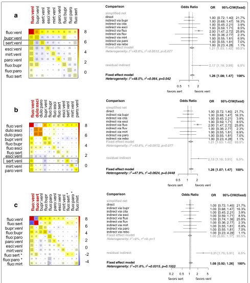
Validation of the sensitivity to perturbations in contrast to the net heat plot approach
To compare the consistency analysis in forest plots of independent paths in contrast to the net heat plot approach, we perturbed chosen direct treatment effects in the constructed, consistent dataset as described above.
At first, we perturbed the direct treatment effect esti-mate of design fluo:venl by inflating the OR by a factor of two. In the net heat plot, this results in an associated red-coloured diagonal element that depicts the contribu-tion of design fluo:venl to the inconsistency in the network (see Figure 4a). Other designs, for example sert:venl, con-tribute to the inconsistency statistic as well, albeit in attenuated form, which can be seen by the correspond-ing yellow-coloured diagonal elements. This is because their network estimates are largely driven by the direct treatment effect of design fluo:venl (see the gray squares in column fluo:venl), and these network estimates are also affected. Inspecting the warm-coloured off-diagonal elements, inconsistency between the direct evidence of designs fluo:venl and bupr:venl as well between fluo:venl and fluo:bupr can be observed. Since only the elements in the column of fluo:venl are coloured the same as the cor-responding diagonal elements, a complete elimination of inconsistency in the whole network is only reached after relaxing the consistency assumption for design fluo:venl.
On the right side of Figure 4a, the forest plot for the network estimate of comparison sert:venl based on the independent path decomposition of Figure 3a is shown. Since we constructed the dataset by setting the OR of all studies to one (with exception of the OR of studies with design fluo:venl in this perturbed case), the network esti-mate for comparison sert:venl, shown by the diamond on the bottom of the forest plot, should be equal to one. But it can be seen that the indirect estimate via fluo (OR: expθfluo:venldir −θfluo:sertdir = exp(log(2)−log(1)) = 2) as well as the pseudo effect estimate of the residual evidence
is affected by the perturbed direct treatment effect esti-mate of design fluo:venl. This, in turn, influences the net-work estimate of comparison sert:venl, since the indirect estimate via fluo comprises 26% of the estimate.
In perturbation setting two, when we perturbed not only the direct treatment effect of design fluo:venl, but also of design dulo:esci to the same extent, we can observe the largest inconsistency contributions in the net heat plot in Figure 4b for these designs as well as for design dulo:paro. The blue-coloured elements in the upper left corner indi-cate that the direct effect of design fluo:venl and that of dulo:esci (or alternatively dulo:paro) support each other. This means the detachment of one of both designs from the network estimation increases the residual of the other design and the inconsistency in the network can be elim-inated in neither of the detachments. Since the adjacent edges corresponding to designs dulo:esci and dulo:paro are part of an essentially non-branching path, the residu-als resulting from the detachment of one of both designs are highly correlated, and the two corresponding columns contains very similarly coloured elements. Because the direct evidence of design dulo:esci drives only a little of the network estimate of comparison sert:venl, which can be seen by the little gray square in column dulo:esci and row sert:venl, the additional perturbation of the effect of design dulo:esci hardly changes the network estimate of comparison sert:venl.
This is duly reflected in the accompanying forest plot. Due to the small contribution of the direct evidence of design dulo:esci to the network estimate of comparison sert:venl, the edge corresponding to design dulo:esci is not part of the subnet that approximates the network esti-mate of comparison sert:venl, and the perturbation is only slightly recognisable in the forest plot by the small change of the residual evidence.
In perturbation setting three, in addition to the direct treatment effect of design fluo:venl, we perturbed the effect of design fluo:sert by inflating the OR by a fac-tor of two. An indirect effect estimate of comparison sert:venl via fluo therefore also results in an OR of 1 as in the unperturbed case (expθfluo:venldir −θfluo:sertdir = exp(log(2)−log(2))= 1). The net heat plot in Figure 4c indicates that both perturbations take effect in the same direction (the direct effects of both designs support each other, as shown by the blue-coloured elements), whereas in the forest plot only a small change in the pseudo effect estimate of the residual evidence is recognisable, and the indirect estimate via fluo is not affected at all. Thus, the forest plot clearly reveals that both perturbations taken together are not relevant for the comparison sert:venl.
a
b
c
plot is selectively sensitive to biases that affect the consid-ered treatment comparison. In contrast the net heat plot summarises the network drivers and inconsistencies in the whole network.
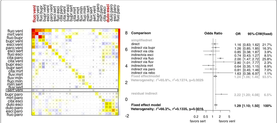
Using the real data of the antidepressants network-meta analysis after perturbing the directly estimated odds ratios for designs fluo:venl and dulo:esci by a factor of two, we can also see that both perturbations are detected by the net heat plot in Figure 5. But as seen in the forest plot for comparison sert:venl, the first one almost exclusively affects the network estimate and the consistency between different evidence sources.
Discussion and conclusions
In network meta-analysis, evidence from different designs contributes to a comparison between two treatments. For the consistency assessment between the effects of differ-ent evidence sources, we have provided a visualisation of an approximating independent path decomposition by forest plots and have investigated its performance in com-parison to that of the net heat plot. We have shown for the example of the highly interconnected network of twelve antidepressants that most network-based treat-ment comparisons are approximated well by the evidence of independent paths. The proposed forest plot discloses and summarises the essentials of a given network-based treatment comparison: the weight given to each path, the consistency between all paths, the comparison between the estimate based on the approximation and on the whole network, and the residual evidence that is not included in the approximation is condensed into a pseudo estimate.
The heterogeneity reported in this forest plot captures these aspects of the inconsistency, which are crucial for the considered comparison.
By perturbing the antidepressants network, after mak-ing it artificially perfectly consistent, we have shown how different kinds of perturbation show up as drivers of inconsistency in the net heat plot or as outlying path-specific evidence in the forest plot. While the net heat plot is sensitive to all kinds of perturbation that sufficiently inflate Cochran’s Q statistic for inconsistency, the forest plot indeed revealed to be selectively sensitive to pertur-bations that are influential to the considered comparison. Independent path approximations should be considered only if they capture, say, more than 80% of the network evidence. If this is not the case, the complete network should be inspected. The flow of evidence can be dis-played as a graph as outlined in [16], and influential designs can be sought for in the net heat plot. A for-est plot that exhibits consistent and balanced evidence from several independent paths and that is additionally in accordance with the residual evidence may indeed be more convincing than a simple meta-analysis of direct comparisons (as similarly argued in [20]).
Paths independence can be defined in two ways, edge independence and vertex independence. In both defini-tions, the path-based effect estimates are uncorrelated. We have applied edge independence. Note that in an edge independent path decomposition, the estimate based on the subnet may be different from the estimate based on the independent paths if some paths share a common inter-mediate vertex. Two paths may contain some common
fluo:paro esci:paro dulo:parodulo:esci cita:esci mirt:paro bupr:paro fluv:sert miln:sertfluo:miln fluv:milnfluv:mirt cita:mirt bupr:sert bupr:escicita:venl cita:parofluo:esci esci:sert paro:venlesci:venl bupr:venlfluo:bupr mirt:venl fluo:venl
fluo:venl mirt:venl fluo:bupr bupr:venl esci:venl paro:venl esci:sert fluo:esci cita:paro cita:venl bupr:esci bupr:sert cita:mirt fluv:mirt fluv:miln fluo:miln miln:sert fluv:sert sert:venl bupr:paro mirt:paro
sert:venl
cita:esci dulo:esci dulo:paro esci:paro fluo:paro
-2 0 2 4 6 8 Comparison
Fixed effect model
Heterogeneity: =66.2%, =0.1335, p=0.0016 simplifiednet
residual indirect Fixed effectmodel
Heterogeneity: =65.8%, =0.1274, p=0.0029 direct
indirect via bupr indirect via cita indirectvia esci indirect via fluo indirect via fluv indirectvia mirt indirect via paro indirect via rebo
Odds Ratio OR
1.29 1.24 2.22 1.16 1.26 0.85 0.74 2.00 2.80 0.64 0.81 1.63 95%-CI [1.10; 1.50] [1.06; 1.46] [1.20; 4.08] [0.83; 1.62] [0.85; 1.85] [0.38; 1.87] [0.43; 1.27] [1.47; 2.72] [1.01; 7.77] [0.35; 1.15] [0.45; 1.46] [0.38; 6.97] W(fixed) 100% 93.5% 6.5% 21.7% 16.3% 3.9% 8.5% 25.8% 2.3% 6.9% 7.0% 1.1%
0.2 0.5 1 2 5 favors sert favors venl
intermediate vertices, and the forest plot implicitly splits these nodes. As a consequence, the subnet has more inconsistency degrees of freedom [10] than the corre-sponding forest plot. For the antidepressants network, on average only 2% of precision is lost by the approximation based on independent paths instead of the subnet.
We focused on the fixed effects model in our exposition, because inconsistency is most easily detectable then [1], but note that the proposed forest plot can be adapted to random effects models by assuming that the heterogene-ity variance is known and fixed and by adding appropriate elements to the covariance matrix of direct effect esti-mates. The heterogeneity variance parameters would have to be assessed using the study level data (see e.g. [21] for various options to model the heterogeneity covariance structure). Then a forest plot is set up for the result-ing independent paths formally usresult-ing the fixed effects option but based on increased variances of the direct effect estimates. Random effects parameters can be esti-mated e.g. via the method of moments, by restricted max-imum likelihood or by Bayesian methods. If the resulting point estimates of heterogeneity variance parameters are plugged in, our diagnostic tools are valuable for all these approaches.
In the literature, various methods have been discussed for the assessment of outliers and influence. In princi-ple, all methods introduced for linear regression [22,23] can be used [2,9]. For network meta-analysis, plots of deviance residuals [24] have been discussed [8] as well plots of squared Pearson residuals [25]. At an aggregate level, regression diagnostics amount to analysis of incon-sistency, with index plots of leverages and residuals [26], concepts like node-splitting [8], and design-by-treatment interaction [12,13]. None of these approaches focuses on the meaning of inconsistency-generating evidence for a specific treatment comparison and none offers all the ana-lytical capacities known from the forest plot in classical meta-analysis for visualising the composition of evidence and identifying potential discrepancies.
Our proposed methods are confined to comparisons that are well-approximated by an estimate based on an independent path decomposition. In complex networks, comparisons that do not fit into this scheme may well be assessed by defining an approximating subnet that is more complex than a decomposable subnet, but much less complex than the whole network. In the antidepressants example more than half of all edges have weights less than 1/44, which is one fourth of the weights seen in a com-plete and balanced network of 12 treatments. Only a few percentages loss in precision should result from omitting these edges. Resorting to a subnet estimate if it captures more than 95% of the evidence for one comparison could be a remedy to the model uncertainty, e.g. with regard to the network size that was discussed in [27].
In conclusion, we have introduced forest plots of independent path decompositions for the assessment of consistency in complex meta-analytic networks as well. We have seen that this graphical presentation known from classical meta-analysis captures the essen-tials of a network-based treatment comparison and dis-closes both the composition of evidence and sources of potential inconsistency relevant for the considered comparison.
Competing interests
The authors declare that they have no competing interests.
Authors’ contributions
UK, HB, and JK developed the methods. UK and JK produced the results and wrote the first draft of the manuscript. All authors read and approved the final manuscript.
Acknowledgements
We thank Katherine Taylor for proofreading.
Author details
1Institute of Medical Informatics, Biometry and Epidemiology, University
Hospital, University Duisburg-Essen, Hufelandstr. 55, 45122 Essen, Germany.
2Institute of Medical Biostatistics, Epidemiology and Informatics, University
Medical Center Johannes Gutenberg University Mainz, Langenbeckstr. 1, 55101 Mainz, Germany.
Received: 7 August 2014 Accepted: 28 October 2014 Published: 16 December 2014
References
1. Salanti G:Indirect and mixed-treatment comparison, network, or
multiple-treatments meta-analysis: many names, many benefits, many concerns for the next generation evidence synthesis tool.
Res Synth Methods2012,3(2):80–97.
2. Dias S, Welton NJ, Sutton AJ, Caldwell DM, Lu G, Ades AE:Evidence
synthesis for decision making4: inconsistency in networks of evidence based on randomised controlled trials.Med Decis Making
2013,33:641–656.
3. Sutton AJ, Higgins JPT:Recent developments in meta-analysis.
Stat Med2008,27:625–650.
4. Lewis S, Clarke M:Forest plots: trying to see the wood and the trees.
BMJ2001,322(7300):1479–1480.
5. Salanti G, Marinho V, Higgins JPT:A case study of multiple-treatments
meta-analysis demonstrates that covariates should be considered.
J Clin Epidemiol2009,62(8):857–864.
6. Dias S, Welton NJ, Sutton AJ, Caldwell DM, Guobing L, Ades AE:NICE DSU
Technical Support Document 4: Inconsistency in Networks of Evidence Based on Randomised Controlled Trials.2011. [http://www.nicedsu.org.uk]
7. Lu G, Ades AE:Assessing evidence inconsistency in mixed treatment
comparisons.J Am Stat Assoc2006,101(474):447–459.
8. Dias S, Welton NJ, Caldwell DM, Ades AE:Checking consistency in mixed
treatment comparison meta-analysis.Stat Med2010,29:932–944.
9. Piepho HP:Network meta-analysis made easy: detection of
inconsistency using factorial analysis-of-variance models.BMC Med
Res Methodol2014,14:61.
10. Krahn U, Binder H, König J:A graphical tool for locating inconsistency
in network meta-analyses.BMC Med Res Methodol2013,13:35. 11. Cipriani A, Furukawa TA, Salanti G, Geddes JR, Higgins JP, Churchill R,
Watanabe N, Nakagawa A, Omori IM, McGuire H, Tansella M, Barbui C:
Comparative efficacy and acceptability of 12 new-generation antidepressants: a multiple-treatments meta-analysis.Lancet2009,
373(9665):746–758.
12. Higgins JPT, Jackson D, Barrett JK, Lu G, Ades AE, White IR:Consistency
13. White IR, Barrett JK, Jackson D, Higgins JPT:Consistency and inconsistency in network meta-analysis: model estimation using multivariate meta-regression.Res Synth Methods2012,3(2):111–125.
14. Caldwell DM, Welton NJ, Ades AE:Mixed treatment comparison
analysis provides internally coherent treatment effect estimates based on overviews of reviews and can reveal inconsistency.
J Clin Epidemiol2010,63(8):875–882.
15. Bucher HC, Guyatt GH, Griffith LE, Walter SD:The results of direct and
indirect treatment comparisons in meta-analysis of randomised controlled trials.J Clin Epidemiol1997,50(6):683–691.
16. König J, Krahn U, Binder H:Visualizing the flow of evidence in network
meta-analysis and characterizing mixed treatment comparisons.
Stat Med2013,32:5414–5429.
17. Dijkstra EW:A note on two problems in connexion with graphs.
Numerische Mathematik1959,1:269–271.
18. Schwarzer G:meta: Meta-Analysis with R.R package version 3.0-1,2013.
[http://CRAN.R-project.org/package=meta]
19. Rücker G, Schwarzer G, Krahn U, König J:netmeta: Network
meta-analysis with R.R package version 0.5-0,2014. [http://CRAN.R-project.org/package=netmeta]
20. Song F, Harvey I, Lilford R:Adjusted indirect comparison may be less
biased than direct comparison for evaluating new pharmaceutical interventions.J Clin Epidemiol2008,61(5):455–463.
21. Lu G, Ades AE:Modeling between-trial variance structure in mixed
treatment comparisons.Biostatistics2009,10(4):792–805.
22. Cook RD, Weisberg S:Residuals and Influence in Regression. New York:
Chapman and Hall; 1982.
23. Belsley DA, Kuh E, Welsch RE:Regression Diagnostics: Identifying Influential
Data and Sources of Collinearity. New Jersey: John Wiley & Sons; 2004.
24. Spiegelhalter DJ, Best NG, Carlin BP, van der Linde, A:Bayesian measures
of model compelxity and fit.J R Stat Soc B2002,64:583–639.
25. Senn S, Gavini F, Magrez D, Scheen A:Issues in performing a network
meta-analysis.Stat Methods Med Res2012,22(2):169–189.
26. Lu G, Welton NJ, Higgins J, White I, Ades A:Linear inference for mixed
treatment comparison meta-analysis: a two-stage approach.
Res Synth Methods2011,2(1):43–60.
27. Sturtz S, Bender R:Unsolved issues of mixed treatment comparison
meta-analysis: network size and inconsistency.Res Synth Methods
2012,3:300–311.
doi:10.1186/1471-2288-14-131
Cite this article as:Krahnet al.:Visualizing inconsistency in network meta-analysis by independent path decomposition.BMC Medical Research Methodology201414:131.
Submit your next manuscript to BioMed Central and take full advantage of:
• Convenient online submission
• Thorough peer review
• No space constraints or color figure charges
• Immediate publication on acceptance
• Inclusion in PubMed, CAS, Scopus and Google Scholar
• Research which is freely available for redistribution