ABSTRACT
GHOSAL, RAHUL. Hypothesis Testing and Variable Selection in Functional Concurrent Regression Model. (Under the direction of Arnab Maity.)
Functional regression is an active area of research in functional data analysis with a vast literature to address problems where the response variable, the predictors, or both are functions over some continuous index such as time. In this dissertation, we develop hypothesis testing and variable selection methods for functional concurrent regression models. Chapter 1 gives a general introduction to functional concurrent regression models and a brief outline of this thesis.
Functional linear concurrent model has been the most frequently used functional concurrent regression model with several applications in longitudinal and spatiotemporal studies. Although there exist multiple methods for estimation in such model, methods for testing the global effect of predictors are relatively few. A novel method for testing the null hypothesis of no effect of a covariate on the response is proposed in Chapter 2. Asymptotic distribution of the test statistic is established under null using standard assumptions. Numerical simulations are used to illustrate the performance of the proposed testing method in terms of type I error rate and power. Applications of the proposed testing method are demonstrated on real data.
In Chapter 3, a method for variable selection is developed for the functional linear concurrent regression model. The work is motivated by a fisheries footprint study, with a goal to select the relevant predictors influencing fisheries footprint over time as well as to estimate their dynamic effects. We extend the classically used scalar on scalar variable selection methods like LASSO, SCAD and MCP for this purpose. Our proposed penalty on the coefficient functions penalizes both their roughness and departure from sparsity. Numerical simulations are provided to illustrate satisfactory selection performance and estimation accuracy of the proposed method. Finally, the proposed method is applied to real data for selection of influential time varying covariates and estimating their concurrent effects.
© Copyright 2019 by Rahul Ghosal
Hypothesis Testing and Variable Selection in Functional Concurrent Regression Model
by Rahul Ghosal
A dissertation submitted to the Graduate Faculty of North Carolina State University
in partial fulfillment of the requirements for the Degree of
Doctor of Philosophy
Statistics
Raleigh, North Carolina 2019
APPROVED BY:
Luo Xiao Eric Chi
Stefano B Longo Arnab Maity
DEDICATION
BIOGRAPHY
ACKNOWLEDGEMENTS
I would like to express my gratitude to my advisor Dr. Arnab Maity for his constant support and guidance throughout my PhD program at NC State and believing in me. Be it my research or mentoring me, he was always just one door knock away. I would like to thank Dr. Luo Xiao and Dr. Eric Chi for being being part of my advisory committee and giving me guidance me both in my research and my career. I would also like to thank Dr. Stefano B Longo for being in my advisory committee and helping me out during our collaboration. I would like to thank Dr. Sujit Ghosh for working with me and mentoring me in realizing my future career goals. I would like to thank Dr. Donald Martin and Dr. Charles Smith for their ever smiling and encouraging presence whenever I met them. I am also very grateful to professors at NC State, Drs. Dennis Boos, Jacqueline Hughes-Oliver, Subhashis Ghoshal, Soumendra Nath Lahiri, Marie Davidian, Donna Barton, Paul Savariappan for their teaching and the example they set. I would like to thank Terry Byron for helping me out with any computing difficulties I faced during my research. I would specially like to thank Alison and Lanakila for being department moms and taking care of us, without them nothing would work. I would like to thank Dr. Debasis Sengupta at Indian Statistical Institute for his guidance and being an inspiration to look up to. I would like to thank Dr. Sedigheh Mirzaei Salehabadi and Timothy Clark for being amazing collaborators to work with. I would like to mention and thank my Mathematics and Statistics teacher at Uttarpara Govt. High School, Mr. Abhijit Sengupta who inspired me and made me fall in love with Mathematics and Statistics.
My time at Raleigh has been a memorable experience thanks to my friends here, who have made this feel a home away from home. I have spent some wonderful time and made some amazing memories with Suman, Indrabati, Sahooda, Golda, Arkopalda, Hazrada, Sohinidi, Moumitadi, Chak, Salilda, Dhrubajyoti (DJG), Priyam (Ala) da, Tuhin, Sukanya, Rahul, Sayak, Abhishekda over the years.
always been there with me in everything. I want to thank her and my two best friends Debarun and Rajit for still keeping the child inside me alive and just being crazy with me in general. I want to thank my friends back home, for just being my friends, the Danesh Eleven (maybe more than eleven); you know who you are, I love you guys and miss you. Lokkhichanas I miss you too.
I want to thank all my relatives and cousins for their love, motivation and support in everything I do. I want to thank my Kaka, Kakima, Pisimoni for their blessings and bhai Arka, who has grown up infront of my eyes and is one of my dearest friend now. I want to mention my grandfather late Shri Gourchandra Ghosal, under whom my education started. I want to remember my grandmother late Smt. Chayarani Ghosal, she was an important part of my growing up. I really miss her.
TABLE OF CONTENTS
LIST OF TABLES . . . .viii
LIST OF FIGURES . . . ix
Chapter 1 Introduction . . . 1
Chapter 2 A Score Based Test for Functional Linear Concurrent Regression . 5 2.1 Introduction . . . 5
2.2 Methodology . . . 8
2.2.1 Modeling framework . . . 8
2.2.2 Equivalent random effects model . . . 9
2.2.3 Testing method . . . 11
2.2.4 Estimation of Covariance Matrix . . . 14
2.2.5 Extension to Sparse and Noisy Covariate . . . 15
2.2.6 Extension to multiple covariates . . . 17
2.3 Simulation Study . . . 18
2.3.1 Study design . . . 18
2.3.2 Simulation Results . . . 19
2.4 Real Data Applications . . . 24
2.4.1 Gait Data . . . 25
2.4.2 Calcium Absorption Data . . . 27
2.5 Discussion and Future Work . . . 29
Chapter 3 Variable Selection in Functional Linear Concurrent Regression . . . 31
3.1 Introduction . . . 31
3.2 Methodology . . . 33
3.2.1 Modeling Framework and Variable Selection Method . . . 33
3.2.2 Incorporating Covariance Structure into variable selection . . . 37
3.2.3 Extension to Sparse data and Noisy Covariates . . . 39
3.3 Simulation Study . . . 40
3.3.1 Simulation Set Up . . . 40
3.3.2 Simulation Results . . . 41
3.4 Real Data Applications . . . 46
3.4.1 Study of Dietary Calcium Absorption . . . 46
3.4.2 Study of Fisheries Footprint . . . 50
3.5 Discussion . . . 57
Chapter 4 Variable Selection in Nonparametric Functional Concurrent Re-gression . . . 59
4.1 Introduction . . . 59
4.2 Methodology . . . 61
4.2.2 Extension to Sparse and Noisy Data . . . 65
4.3 Simulation Study . . . 66
4.3.1 Simulation Set Up . . . 66
4.3.2 Simulation Results . . . 67
4.4 Real Data Applications . . . 71
4.4.1 Study of Dietary Calcium Absorption . . . 71
4.4.2 Study of Bike Sharing Data . . . 73
4.5 Discussion . . . 77
Chapter 5 Conclusion . . . 79
BIBLIOGRAPHY . . . 81
APPENDIX . . . 86
Appendix A Proofs and Additional Results . . . 87
A.1 Proof of Theorem 1 . . . 87
A.2 Proof of Theorem 2 . . . 88
LIST OF TABLES
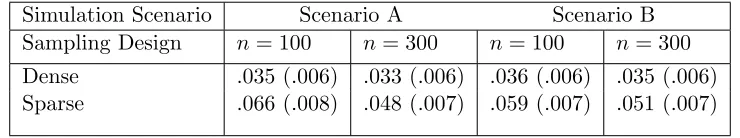
Table 2.1 Estimated type I error along with their standard error atα= 5% level. . . 20
Table 3.1 Comparison of selection percentages (%) of different variables and average model size, without pre whitening. . . 43
Table 3.2 Comparison of selection percentages (%) of different variables and average model size, with pre whitening. . . 44
Table 3.3 Comparison of MC absolute bias and mean square error. . . 45
Table 3.4 Selection Percentages (%) of variables in Calcium absorption Study. . . 48
Table 3.5 List of covariates in the Fisheries Footprint Study. . . 52
Table 4.1 Comparison of selection percentages (%) of different variables and mean model size, Scenario A. . . 68
Table 4.2 Quantiles of out of sampleR2M ed based on MC simulation, Scenario A. . . 69
Table 4.3 Comparison of selection percentages (%) of different variables, Scenario B. 70 Table 4.4 Quantiles of out of sampleR2M ed based on MC simulation, Scenario B. . . 71
Table 4.5 Selection Percentages (%) of variables in Calcium absorption Study using NPFCM. . . 73
LIST OF FIGURES
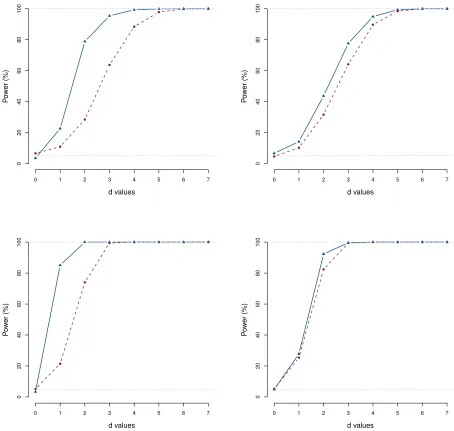
Figure 2.1 Results of simulation study as described in Section 2.3, Scenario A. Dis-played are the power curves for our proposed procedure (solid line) and the bootstrap-F test based method (dashed line) for dense (left column) and sparse (right column) sampling designs with sample sizes n = 100 (top row) andn= 300 (bottom row). . . 21 Figure 2.2 Power curve for simulation Scenario A, additional simulation study, n=39,
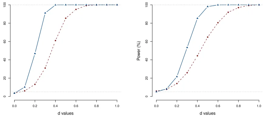
m=20. . . 22 Figure 2.3 Results of simulation study as described in Section 2.3, Scenario B.
Dis-played are the power curves for our proposed procedure with sample sizes
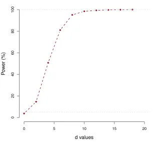
n= 100 (dashed line) and n= 300 (solid line) for dense (left column) and sparse (right column) sampling designs. . . 23 Figure 2.4 Effect of number of basis on the power of the test, simulation Scenario A,
n=300. . . 24 Figure 2.5 Measurement of hip angles and knee angles in the gait study. . . 25 Figure 2.6 Results from simulation study mimicking gait data. Displayed is the power
curve of our test. . . 27 Figure 2.7 Observed calcium absorption and calcium intake in the calcium absorption
study. . . 28 Figure 3.1 MC estimates and point wise confidence intervals of the coefficient functions
(n=200). . . 42 Figure 3.2 Calcium absorption and covariate profiles of patients along their ages. . . 47 Figure 3.3 Bootstrap estimate and point wise confidence interval of the the effect of
calcium intake (left panel) and percentage observation available in different age groups (right panel). . . 49 Figure 3.4 Fisheries footprint of the nations over year 1970-2009. . . 52 Figure 3.5 Mean fisheries footprint along with their 95% confidence interval. . . 53 Figure 3.6 Estimate of the linear concurrent effect of GDP per capita on fisheries
footprint (SCAD). . . 54 Figure 3.7 Estimate of the linear concurrent effect of urban population on fisheries
footprint (SCAD). . . 55 Figure 3.8 Profile of fisheries footprint, GDP per capita and urban population of
three representative countries. . . 56 Figure 4.1 Estimate of non-parametric effect of calcium intake on calcium absorption
from proposed variable selection method in NPFCM. . . 73 Figure 4.2 Hourly casual Bike rentals and weather variables profile in bike sharing data. 74 Figure 4.3 Estimated non-parametric concurrent effect of the weather variables.
Chapter 1
Introduction
literature in functional linear concurrent regression model regarding estimation of the regression functions; using kernel-local polynomial smoothing (Wu et al., 1998; Hoover et al., 1998; Fan and Zhang, 1999; Kauermann and Tutz, 1999), polynomial spline (Huang et al., 2002, 2004), smoothing splines (Hastie and Tibshirani, 1993; Hoover et al., 1998; Chiang et al., 2001; Eubank et al., 2004) among many others. Estimation of the regression functions is important as they can reveal the time varying effect the predictors have on the response.
Extending the functional linear concurrent model (FLCM) is the nonparametric or general functional concurrent model which overcomes the assumption of linear dependence between response and covariates in FLCM; which may not be true in many real data applications, by specifying a nonparametric relationship, which is more general and flexible for modeling purposes. Here also, there exists multiple methods for estimation such as smoothing splines (Kim et al., 2018), Gaussian process regression (Shi et al., 2005), local kernel smoothing techniques (Jiang et al., 2011), etc. For non-Gaussian functional responses, an extension of the nonparametric functional concurrent model is the generalized functional concurrent model of Wang and Shi (2014).
While several methods for estimation and prediction are available in the literature for the functional linear concurrent model (FLCM) or the nonparamteric functional concurrent model (NPFCM), methods for testing of global effects of covariates and methods for variable selection are relatively few, specially in the context of function on function regression models. In this dissertation, therefore, the focus has been to develop methods for hypothesis testing and variable selection in the context of functional concurrent regression models.
test. We establish asymptotic distribution of our test statistic under null and provide theoretical justification as to why our testing procedure has the right levels (asymptotically) under null using standard assumptions. Using numerical simulations, we show that our testing method has the desired type I error rate as well as a higher power than a standard bootstrapped F test used in the literature. Our model and testing procedure are shown to give good performances even when the data is sparsely observed, and the covariate is contaminated with noise. We also demonstrate application of our method on real data.
In Chapter 3, we develop a method for variable selection in functional linear concurrent regression. Our research is motivated by a fisheries footprint study where one of the goals is to identify important time varying socio-structural drivers influencing patterns of seafood consumption and hence fisheries footprint over time. We develop a variable selection method in functional linear concurrent regression extending the classically used scalar on scalar variable selection methods like LASSO, SCAD and MCP. We show in functional linear concurrent regression the variable selection problem can be addressed as a group LASSO, and their natural extension; group SCAD or a group MCP problem. Through simulations, we illustrate our proposed method, particularly with group SCAD or group MCP penalty can pick out the true underlying variables with high accuracy and has minimal false positive and false negative rate. Finally, we apply our method in a study of dietary calcium absorption and fisheries footprint, for selection of influential time varying covariates.
selection accuracy and out of sample prediction performance. Real data applications on a dietary calcium absorption study and a bike sharing data demonstrate the proposed method can be used successfully for variable selection while simultaneously estimating nonparametric concurrent effect of the predictors which helps to understand underlying dynamics between the response and the predictors.
Chapter 2
A Score Based Test for Functional
Linear Concurrent Regression
2.1
Introduction
be finding out whether a specific covariate is truly significant or not, i.e., to test for association between a predictor of interest and the response. For example, in the gait study data (Ramsay and Silverman, 2005), where there are longitudinal measurements of hip and knee angles taken on 39 children, the main purpose of the study is to understand how the joints in hip and knee interact during a gait cycle (Theologis, 2009). One natural question to ask here would be, whether the knee angles (response) are at all associated with the hip angles (covariate). Simply building a point-wise confidence interval of the estimated regression function does not answer the question of the overall significance of the covariate. Thus there is a need for developing testing methods to find out significant predictors in this setting.
Formally, our primary goal is to test the null hypothesis that the coefficient function corresponding to a predictor of interest is identically zero, versus the alternative hypothesis that the coefficient function is non-zero for some time point. Literature relating to such global testing in functional concurrent linear regression or closely related varying coefficient model can be traced back to Huang et al. (2002), Guo (2002) among many others. Huang et al. (2002) employed a resampling subject bootstrap method on an F-type statistic, whereas Guo (2002) used the connection between linear mixed effects models and smoothing splines, and subsequently used a generalized maximum likelihood ratio test to test for significance of predictors. Kim et al. (2018) extended the bootstrap based test (Huang et al., 2002) to general nonlinear functional
concurrent model. Both of these tests rely on a subject-level bootstrap method to obtain the p-values making the test computationally intensive. Recently, Wang et al. (2018) developed a method for pointwise as well as global testing using empirical likelihood ratio tests. Their method, which is extremely general, uses a wild bootstrap procedure to perform the test for both dense and sparse functional data. Besides these global testing procedures one can also use confidence bands based methods e.g., Fan and Zhang (2000) for building simultaneous confidence bands for the underlying coefficient functions.
regression coefficients using B-spline basis functions and derive an equivalent random effects model. Under such a framework, we show that our testing problem reduces to testing for zero variance components for a set of random effects. There are multiple existing methods in the literature for testing for zero variance components. Crainiceanu and Ruppert (2004), Greven et al. (2008), and Staicu et al. (2014) considered testing for variance components using likelihood ratio test (LRT) and restricted likelihood ratio test (RLRT). The main challenge of such tests is that the null distribution is different from the commonly used 0.5χ20 : 0.5χ21 approximation or such mixtures of two chi-square distributions, which is used in Guo (2002). In this article, we propose a score based testing method that is computationally efficient. Our procedure is inspired from the work of Molenberghs and Verbeke (2007) which describes an approach of using a one-sided score test in constrained parameter space. The major advantage of working with the score test is, it does not require computations under the alternative. Zhang and Lin (2008) and Lin (1997) also used such one-sided score tests for variance component testing in generalized linear mixed models and longitudinal data. However, the methods mentioned above assumed that the responses are independent given the random effects and that the variances have some parametric form. In contrast, in our functional regression framework, we assume unknown non-trivial covariance structure and estimate the covariance function nonparametrically. The assumption of non-trivial dependence is crucial in functional data because of complex correlation structures that might be present in real data. We derive the asymptotic distribution of the test statistic under the null hypothesis; we show that the commonly used chi-squared approximation of the score test statistic is not appropriate in our situation. However, the null distribution of our test statistic is easy to simulate from. Thus the calculation of p-value for our testing procedure is computationally efficient. We show that asymptotically our testing procedure has the correct type I error rate. Using numerical simulations, we illustrate that our testing method has the desired type I error rates for finite sample sizes and that our proposed testing procedure has higher power than the bootstrapped F-test of Kim et al. (2018).
present our testing method and derive theoretical properties related to our test statistic. In Section 2.3, we present a simulation study under various sampling design scenarios and give the simulation results. In Section 2.4, we demonstrate our proposed test by applying it to the two real data examples: gait data and calcium absorption study and summarize our findings. We conclude by a discussion about some limitations and some possible extensions of our work in Section 2.5.
2.2
Methodology
2.2.1 Modeling framework
Suppose that the observed data for the ith subject, i= 1, . . . , n, is {Yi(t), Xi1(t), . . . , Xip(t)}, where Y(·) is a functional response andX1(·),. . . , Xp(·) are the corresponding functional covari-ates. In practice, the functions for theith subject are observed only on a finite set of pointstij,
j= 1, . . . , mi. We assume thattij ∈ T, a bounded and closed set. For the rest of the article, we assume T = [0,1] without loss of generality. To start with, we will assume that tij =tj, and that the covariates Xik(·) are measured without error. We discuss the cases when the functions are observed on irregularly spaced grid, and with additional measurement errors in Section 2.2.5. We consider a functional linear concurrent regression model,
Yi(t) =β0(t) + p X k=1
Xik(t)βk(t) +i(t),
where β0(t) and βk(t) (k= 1,2, . . . , p) are smooth functions representing functional intercept and functional slope parameters, respectively. We assumeXik(·) are independent and identically distributed (i.i.d.) copies ofXk(·) (k= 1,2, . . . , p), where Xk(·) is a stochastic processes with finite second moment. For simplicity we illustrate our testing method for the single covariate model
which can be easily extended to the multiple covariate situation above and this is discussed in Section 2.2.6. We further assume i(·) are i.i.d. copies of (·), which is a mean zero Gaussian process plus some Gaussian white noise, that is, (t) =V(t) +wt,whereV(·)∼ N(0, G(·,·)) andwt are i.i.d. N(0, σ2) random errors. Thus the covariance function of the error process is given by Σ(s, t) =cov((s), (t)) =G(s, t) +σ2I(s=t). Our primary interest lies in testing,
H0 :β1(t) = 0 for allt versus H1:β1(t)6= 0 for some t.
In general, testingH0 is difficult sinceβ1(t) is an infinite dimensional parameter. In this article we show that by modeling the coefficient function with splines and using a random effects model, the testing problem can be reduced to a variance component test. This reduction in parameter dimension not only helps in getting satisfactory performance of our testing method but also is computationally cheaper than doing the bootstrapped F test existing in literature. Subsequently we develop a one sided score test for testing our null hypothesis.
2.2.2 Equivalent random effects model
An usual method (Ramsay and Silverman, 2005) to estimateβ0(t) andβ1(t) in model (1) is by minimizing the penalized residual sum of squares,
n X i=1
||Yi(·)−β0(·)−Xi(·)β1(·)||2F2 +λ0 Z
{β0r(t)}2dt+λ1 Z
{β1r(t)}2dt,
where λ0, λ1 are unknown penalty parameters penalizing r-th derivative of the coefficient functions and || · ||F2 denotes the functional L2 norm. Suppose for ` = 0,1 {Bk`(t), k = 1,2, . . . , k`} is a set of known basis functions. We write the unknown coefficient functions using basis function expansion as β`(t) =
PK`
k=1bk`Bk`(t) =BT`(t)b`, `= 0,1, whereB`(t) = [B1`(t), B2`(t), . . . , BK``(t)]
T and b
` = (b1`, b2`, . . . , bk``)
[Xi(t)B11(t), Xi(t)B21(t), . . . , Xi(t)Bk11(t)]T. We can then rewrite our model (1) as Yi(t) =
BT0(t)b0+Xi∗T(t)b1+i(t). The unknown basis coefficients can then be estimated by minimizing the penalized error sum of squaresPn
i=1||Yi(·)−BT0(·)b0−X∗iT(·)b1||22+λ0bT0P0b0+λ1bT1P1b1, where P0 and P1 are the penalty matrices coming from penalizing the r-th derivative of the functions β0(t) andβ1(t). In particularP` =RBr`(t)Br`(t)Tdt and thusR(β`r(t))2dt=bT`P`b`. Since we only observe data on a fine regular gridS ={t1, t2, . . . , tm}in practice, the minimization is carried out by minimizing
n X i=1
m X j=1
{Yi(tj)−BT0(tj)b0−X∗i
T
(tj)b1}2+λ0b0TP0b0+λ1bT1P1b1.
DefineYi = [Yi(t1), Yi(t2), . . . , Yi(tm)]T,B0 = [B0(t1)|B0(t2)|. . .|B0(tm)]T,Xi= [X∗i(t1)|X∗i(t2)|
. . .|X∗i(tm)]T.Thus the least square criterion for estimation is given by,
n X
i=1
||Yi−B0b0−Xib1||22+λ0bT0P0b0+λ1bT1P1b1.
Now since the matrices P0,P1 are singular (for r ≥ 1), the equivalent random effects model corresponding to this minimization problem would be rank deficient. As our primary interest lies in testing, we propose to penalize the coefficient functions directly, namely we use r= 0 and consequentlyP` =RB`(t)B`(t)Tdt. Our simulations show we are able to maintain correct type I error rates of the proposed testing method using this strategy. It then follows that the normal equations are identical to those from the equivalent random effects modelYi =B0b0+Xib1+ζi, whereζi∼ Nm(0, σ2Im),b0 ∼ Nk0(0, σ20Σ0),b1 ∼ Nk1(0, σ12Σ1) andb0,b1,ζi are independent. We denote Σ0 = P−01,Σ1 =P
−1 1 , σ02 =
σ2
λ0, σ 2 1 =
σ2
λ1. Using Cholesky decomposition of Σ0,Σ1 and appropriately reparameterizing (C0 = B0Σ1/20 , Zi = XiΣ
1/2
1 , γk = Σ
−1/2
k bk), the model
can be rewritten as Yi = C0γ0 +Ziγ1 +ζi, where ζi ∼ Nm(0, σ2Im), γ0 ∼ Nk0(0, σ20Ik0), γ1∼ Nk1(0, σ12Ik1), and all the random effects are independent. Thus our testH0 can be carried out via testing of a single variance component, namely testingH0 :σ12= 0 against the alternative
Now for our testing problem since the errors are not independent, to get the correct likelihood we need to use the true covariance kernel Σ(s, t) for the residual vectoris, which motivates us to use the random effects model
Yi =C0γ0+Ziγ1+i, (2.2)
wherei ∼ Nm(0,Σm×m),γ0 ∼ Nk0(0, σ20Ik0),γ1 ∼ Nk1(0, σ12Ik1) and all of them are independent. Here Σm×m denotes the covariance kernel Σ(s, t) evaluated at S = {t1, t2, . . . , tm}. For the moment let us assumeΣm×m to be known. Of course in realityΣm×m will be unknown and we will need to estimate it. We illustrate in Section 2.2.4 how to estimate Σm×m using functional principal component analysis (FPCA). Writing equation (2.2) in stacked form fori= 1,2,3, . . . , n
we have
Y =Bγ0+Zγ1+E, (2.3)
where B = [CT0|CT0|. . .|CT0]T, Z = [ZT1|ZT2|. . .|ZTn]T, Y = (YT1,Y2T, . . . ,YnT)T and E = (T1,T2, . . . ,Tn)T.E ∼ NN(0,Σ) (N =mn), where the covariance matrix Σis given byΣ=diag
{Σm×m,Σm×m, . . . ,Σm×m}. Note that Z=XΣ1/21 andB=BΣ 1/2
0 , where X,B are defined simi-larly by stacking Xi andB0 s. So in this set up, we are interested in testingH0 :σ12 = 0 against the alternativeH1:σ21 >0.
2.2.3 Testing method
We develop our testing method treatingZas nonrandom (fixed). Namely our test is a conditional test based on observed Z{i.e., observed Xi(t)}. We show that our conditional testing method has the right levels under null which in turn ensures the unconditional test would also enjoy this property. Marginally Y∼ N(0,V), which follows from equation (2.3) withV=V(τ0, τ1) = Σ+τ0BBT +τ1ZZT, whereτ0 =σ02 and τ1 =σ21. So the marginal log-likelihood of Y (upto a constant) is :
Based on this likelihood, we want to test H0 :τ1 = 0 vsH1 :τ1>0.
Let θ= (τ0, τ1)T and ˜θ denote the maximum likelihood estimate (M.L.E) of θ under H0. The score function of τ1 is
Sτ1(τ0, τ1) =−1/2{tr(V−1M)−YTV−1MV−1Y}
=−1/2{tr(ZTV−1Z)−(V−1/2Y)TV−1/2ZZTV−1/2(V−1/2Y)},
where M = ZZT. The information matrix I(θ) corresponding to the likelihood in (2.4) is partitioned as,
I(θ) =
I11(θ) I12(θ)
I21(θ)T I22(θ)
,
where I11(θ) =tr{(BTV−1B)2}/2, I22(θ) =tr{(ZTV−1Z)2}/2,I21(θ) =I12(θ) =tr{(BTV−1Z) (BTV−1Z)T}/2. Then the classical score test statistic is given by,
TS =
Sτ12 ( ˜θ)
I22( ˜θ)−I21( ˜θ)TI−1
11( ˜θ)I12( ˜θ)
.
As the parameter space is constrained and the null hypothesis is on the boundary of the parameter space, following Molenberghs and Verbeke (2007) we define our one sided score test statistic as
TS =
S2
τ1( ˜θ)
Λ( ˜θ) ifSτ1( ˜θ)≥0
0 ifSτ1( ˜θ)<0,
(2.5)
where Λ( ˜θ) =I22( ˜θ)−I21( ˜θ)TI11−1( ˜θ)I12( ˜θ). We assume the true covariance matrix Σ to be known for the time being for establishing asymptotic distribution of our test statistic but in reality it is generally unknown, so we will need to estimate it from data by some consistent estimator ˆΣ and plug that in forΣ inTS. Next we posit two theorems regarding distribution our test statistic.
a) The null hypothesis is true i.e., H0 :τ1 = 0 holds and θ0 = (τ0∗,0)is the true value of θ,
b) Σ be the true covariance matrix of the residual vectorE in equation (2.3).
Then TS(θ0,Σ) = S 2
τ1(θ0)
Λ(θ0) I(Sτ1(θ0)≥0) d = (1/2)2
Pk1
`=1λ`x2`−
Pk1
`=1λ`
2
Λn(θ0) I(
Pk1
`=1λ`x2` ≥ Pk1
`=1λ`),
where x` iid
∼ N(0,1) and λ` are eigenvalues of ZTV(θ0,Σ)−1Z/n andΛn(θ0) = Λ(θ0)/n2 = 12tr{(ZTV−1Z/n)2}- [
1 2tr{(B
T
V−1Z/n)(BTV−1Z/n)T}]2
1 2tr{(BTV
−1
B/n)2}
The proof of the Theorem 1 is given in Appendix A.1.
Theorem 2. Suppose the following conditions are true :
a) The null hypothesis is true i.e H0 :τ1 = 0 holds and θ0 = (τ0∗,0)is the true value of θ,
b) θ˜is√nconsistent estimator of θ0 under null and the estimatorΣˆ is a consistent estimator of Σ in the sense||Σˆ−1−Σ−1||2 =op(1) (spectral norm).
Then TS( ˜θ,Σˆ) d
→TS(θ0,Σ).
The proof is mainly based on application of Slutsky’s theorem and matrix norm inequalities. A detailed proof is given in Appendix A.2. As mentioned in Theorem 1 the null distribution of the test statistic is given by (1/2)2
Pk1
`=1λ`x2`−
Pk1
`=1λ`
2
Λn(θ0) I(
Pk1
`=1λ`x2` ≥ Pk1
`=1λ`). Becauseθ0 andλ` are unknown in reality, we approximate the null distribution using plug-in estimates of ˜θ and ˆΣ, i.e, we use the approximate null distribution
(1/2)2
Pk1
`=1λ˜`x2` − Pk1
`=1λ˜` 2 Λn( ˜θ)
I( k1 X `=1
˜
λ`x2` ≥ k1 X `=1
˜
λ`), (2.6)
where ˜λ` are eigenvalues of ZTV( ˜θ,Σˆ)−1Z/n and x` iid
∼ N(0,1) for ` = 1,2, . . . , k1. This is justified as it can be shown ˜λ`
p
→ λ` and Λn( ˜θ) p
ZTV( ˜θ,Σˆ)−1Z/n, and simulate x` iid
∼ N(0,1) for`= 1,2, . . . , k1. For calculation of V( ˜θ,Σˆ)−1, we use the Woodbury matrix identity and also the fact ˆΣ is block diagonal, which greatly speeds up the calculation. It is well known (Zhang and Lin, 2003), that the usual asymptoticχ2
distribution of the score test do not work here, so the approximate null distribution in (6) is more appropriate. As the test statistic is one sided and in particular not continuous at zero, the p-value under null is asymptotically distributed as mixture distribution of degenerate one and
U(0, α), whereα=PH0{Sτ1(θ0)≥0}=P(Pk1`=1λ`x2` ≥ Pk1
`=1λ`), a detailed proof is given in Appendix A.3. As k1 increases it follows by application of CLT,α→ 12 and the null distribution of our test statistic asymptotically converges to 0.5χ20 : 0.5χ21. In reality choice of k1 will depend on the type of design (dense or sparse) and number of observed time points for each subjects. So such a convergence need not hold for subjects observed only on a finite set of points. Therefore, we use the approximate null distribution (2.6) to perform our test.
2.2.4 Estimation of Covariance Matrix
In realityΣis unknown, and we need a consistent estimator ˆΣ. In the context of functional data, we want to estimate Σ(·,·) completely non-parametrically. If we had the original residualsij available, we could use functional principal component analysis (FPCA), e.g., Yao et al. (2005) or Zhang et al. (2007) to estimate Σ(s, t). The error process(t) was defined as (t) =V(t) +wt. We assume the covariance kernel G(s, t) of the smooth part V(t) is a Mercer kernel (Mercer, 1909). Then by Mercer’s theoremG(s, t) must have a spectral decomposition
G(s, t) =
∞
X k=1
λkφk(s)φk(t),
where λ1≥λ2 ≥. . .0 are the ordered eigenvalues andφk(·)s are corresponding eigenfunctions. Thus we have Σ(s, t) =P∞
k=1λkφk(s)φk(t) +σ2I(s=t). Giventij =V(tij) +wij, one could
the sparse and dense functional data setting under appropriate regularity conditions on the sampling design. Li and Hsing (2010) established uniform convergence rates for eigenfunctions and eigenvalues under more general framework where the number of observations for each function can be sampled at any rate relative to the sample size. More specifically Li and Hsing (2010) showed it is possible to get consistent estimators ˆφk(·), ˆλk and ˆσ2 under both sparse and
dense functional data settings. So a consistent estimator of Σ(s, t) can be formed as
ˆ
Σ(s, t) = K X k=1
ˆ
λkφˆk(s) ˆφk(t) + ˆσ2I(s=t),
where K is large enough for the convergence to hold and is typically chosen such that percent of variance explained (PVE) by the selected eigencomponents exceeds some pre-specified value such as 99% or 95%. In reality we don’t have the original residualsij and use the full model (1) to obtain residualseij =Yi(tj)−Yˆi(tj). Then treatingeij as our original residuals, we obtain
ˆ
Σ(s, t) using FPCA. Our simulations show good results using this approach and we are able to maintain the correct levels of the test under both sparse and dense sampling design scenarios.
2.2.5 Extension to Sparse and Noisy Covariate
In developing our method we assumed that covariates are measured without noise and data is observed on a regular dense grid of points S={t1, t2, . . . , tm} ⊂ T = [0,1]. Although in reality data might be observed sparsely, and the covariates may be contaminated with measurement error. Our testing method can be extended to these situations in the following ways.
Case 1: Sparse design, no measurement error
We assume response Yi(t) and the covariate Xi(t) are observed in Si = {ti1, ti2, . . . , timi} ⊂
T = [0,1] for each i= 1,2, . . . , n and max1≤i≤nmi ≤M, for some fixed M. In this case the only difference in our model is that Yi is a mi×1 dimensional vector and thati ∼ Nmi(0,Σi)
our model described in (2.2) still holds with Σ=diag{Σ1,Σ2, . . . ,Σn}. As discussed in Section 2.2.4, if Σ(s, t) can be consistently estimated by ˆΣ(s, t) then ˆΣi would be a consistent estimator of Σi and our testing method is still valid.
Case 2: Dense design with measurement error
Suppose now dataYi(t) and covariateXi(t) are observed in a fine regular gridS ={t1, t2, . . . , tm} ⊂ T = [0,1] and the covariate is observed with measurement error. Namely instead of observing
Xi(tj) we observe Uij =Xi(tj) +δij, where δij are i.i.d. mean zero random errors with variance
κ2. There exists several methods to reconstruct the original curveXi(·) from the observed curve with measurement error. Zhang et al. (2007) proposed to use local polynomial kernel smoothing technique for individual function reconstructions. They showed that under appropriate conditions and suitable choice of bandwidth, the smoothed trajectories, ˆXi(·) will estimate the true curves
Xi(·) with negligible error. Thus we can use the reconstructed curves ˆXi(·) and the effect of such a substitution is asymptotically negligible.
Case 3 : Sparse design with measurement error
More generally, we consider the case where functional data is observed in irregular and sparse grid of points and covariate is observed with measurement error. Here we have observed response {(Yi(tij), tij), j = 1,2, . . . , mi} and observed covariate {(U(tij), tij), j = 1,2, . . . , m1i}. Again we assume that Uij =Xi(tij) +δij, whereδij are i.i.d. mean zero random errors with variance
and eigenfunctions for both dense and sparse design under suitable regularity conditions. For prediction of the scores Yao et al. (2005) introduced the PACE method which ensures the estimated scores asymptotically goes to BLUP of the original scores. Then these estimates can be put together using Karhunen-Lo`eve expansion to get estimates ˆXi(·) of the true curve Xi(·). We again use the PVE criterion to select the number of PC. So for sparse data observed on irregular grid and observed with measurement error, we employ FPCA to get ˆXi(t) and then use{Yi(tij),Xˆi(tij), j= 1,2, . . . , mi}ni=1 as our original data to perform our proposed test. Our simulations show that we are able to maintain correct type I error rate and obtain satisfactory power of our testing method using this strategy.
2.2.6 Extension to multiple covariates
Here, we illustrate how our testing method can also be applied in multiple covariate setting. In this case the likelihood is as in (2.4) and given by
LM L(τ0, τ1, . . . , τp) =−1/2(ln|V|+YTV−1Y), (2.7)
with the only difference being V = V(τ0, τ1, . . . , τp) = Σ+τ0BBT +τ1Z1ZT1 +. . .+τpZpZTp. So testing for the effect ofXp(·) here similarly reduces to testing for the variance component
τp, namely, we test H0 :τp = 0 vs H1 :τp >0. The score function Sτp(τ0, τ1, . . . , τp) and the
information matrixI(θ) {θ= (τ0, τ1, . . . , τp)T}are also modified accordingly taking into account the additional variance components, e.g., the information matrix I(θ) now has to be partitioned as
I(θ) =
I11(θ)p×p I12(θ)p×1
I21(θ)T1×p I22(θ)1×1
.
Section 2.3 and real data application in Section 2.4, where we have considered two covariate scenarios and tested for effect of one covariate in presence of other.
2.3
Simulation Study
2.3.1 Study design
In this section, we investigate the performance of our testing method via simulation study. We evaluate our test in terms of type I error rate and power. We also compare our method to the existing bootstrapped F-test proposed by Kim et al. (2018). To this end, we consider the following two scenarios.
Scenario A (single covariate): We generate data from the model,
Yi(t) =β0(t) +Xi(t)β1(t) +i(t),
where β0(t) = 1 + 2t+t2 and β1(t) = t/8. The original covariate Xi(·) are i.i.d. copies of
X(·), where X(t) = a+b√2sin(πt) +c√2cos(πt), where a ∼ N(0,1), b ∼ N(0, .852) and
c∼ N(0, .702) and they are independent. As discussed in Section 2.2, we assume that we observe
Xi(t) with measurement error, i.e., we observeUi(t) =Xi(t) +δ, whereδ∼ N(0, .62). The error processi(t) is generated as
i(t) =ξi1 √
2cos(πt) +ξi2 √
2sin(πt) +N(0,0.92Imi),
where ξi1 iid
∼ N(0,2) and ξi2 iid
∼ N(0,0.752). We consider the following sampling designs:
• Dense design: Functional data are observed in S for each subject, whereS is the set of
m= 81 equidistant time points inT = [0,1].
• Sparse design: The response Yi(t) and noisy covariate Ui(t) both are observed in ran-dom mYi and mUi points in S where mYi
iid
∼ U nif orm{20,21, . . . ,31} and also mUi
U nif orm{20,21, . . . ,31}.
We consider two sample sizes, n= 100 and 300 for comparison with the bootstrapped F test method. An additional simulation is done in this same set up for dense data with m = 20,
n= 39 to illustrate the performance of the testing method for small sample size, as considered in the application section of this article.
Scenario B (Multiple Covariates): We generate data from the model,
Yi(t) =β0(t) +Xi1(t)β1(t) +Xi2(t)β2(t) +i(t),
whereβ0(t) = 1 + 2t+t2, β1(t) =t/8 andβ2(t) =sin(πt). The original covariatesXik(·) are i.i.d. copies ofXk(·), whereXk(t) =ak+bk
√
2sin(πt) +ck √
2cos(πt), whereak∼ N(0,(2−.5(k−1))2),
bk ∼ N(0,(0.85×2−.5(k−1))2), and ck ∼ N(0,(0.70×2−.5(k−1))2), and they are independent. The covariates Xk(·) are same as considered in Kim et al. (2018). We observe Xik(t) with measurement error, i.e., we observeUik(t) =Xik(t) +δk, whereδk∼ N(0, .62). The error process
i(t) are generated as in Scenario A described above. Similar sparse and dense design settings and sample sizes n∈ {100,300} are considered. Here the main goal is to test H0 :β2(t) = 0 against the alternativeH1 :β2(t)6= 0. For each of the scenarios we use 1000 generated data sets to asses type I error and power. To model the regression functions, 12 cubic B-splines are used for all scenarios.
2.3.2 Simulation Results
Scenario A:
We first assess type I error of the test. We use nominal a level of α = 5% for n= 100 and
Table 2.1 Estimated type I error along with their standard error atα= 5% level.
Simulation Scenario Scenario A Scenario B
Sampling Design n= 100 n= 300 n= 100 n= 300
Dense .035 (.006) .033 (.006) .036 (.006) .035 (.006) Sparse .066 (.008) .048 (.007) .059 (.007) .051 (.007)
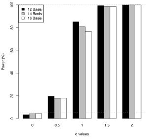
be due to using a small number of basis functions (12) for dense design (m= 81 ). For sparse design, as sample size increases, the size performance of our test improves, which is expected as our test is a large sample one and for the asymptotic convergence to the null distribution to hold we need larger sample size. The nominal level lies within two standard error limit of estimated type I error in this case.
Next, we study the power performance of our test for a fixed nominal level ofα= 5%. To this end, we generate data in the simulation set up mentioned earlier withβ1(t) =dt/8. Thend= 0 corresponds to the null hypothesis and d >0 captures the departure from the null hypothesis. We compare the power of our test to the bootstrapped-F test forn∈ {100,300}, and both dense and sparse sampling designs. For comparison of power with the bootstrapped method, we use the results from the simulation study conducted by Kim et al. (2018). The results of our study are displayed in Figure 2.1.
We note that across the sparse and dense design scenarios, our method produces higher power than the bootstrapped-F test method. This is expected as our method is a likelihood based method. We also observe that as the sample size increases ordincreases the power of our test converges to one across all the settings faster than the bootstrapped-F test. Similar results for the additional simulation study is provided in Figure 2.2.
Scenario B:
0 1 2 3 4 5 6 7
0
20
40
60
80
100
d values
P
o
w
er (%)
0 1 2 3 4 5 6 7
0
20
40
60
80
100
d values
P
o
w
er (%)
0 1 2 3 4 5 6 7
0
20
40
60
80
100
d values
P
o
w
er (%)
0 1 2 3 4 5 6 7
0
20
40
60
80
100
d values
P
o
w
er (%)
Figure 2.1 Results of simulation study as described in Section 2.3, Scenario A. Displayed are the
for n= 100 and n= 300 are considered. Again we observe our test maintaining nominal type I error, and improvement in size performance with increasing sample size, particularly for sparse design. A similar evaluation of power performance is done as in Scenario A. Namely we generate data as in simulation Scenario Bwithβ2∗(t) =dβ2(t). The power curve of our testing method for both dense and sparse settings forn∈ {100,300}are displayed in Figure 2.3. We observe the power converging to one, as sample size or dincreases, across all the sampling designs.
Our simulation results illustrate the proposed testing method is able to maintain the nominal type I error rate as well as capture the departure from null hypothesis efficiently even when data is observed sparsely and the covariates are observed with measurement error.
0 5 10 15 20
0
20
40
60
80
100
d values
P
o
w
er (%)
0.0 0.2 0.4 0.6 0.8 1.0
0
20
40
60
80
100
d values
P
o
w
er (%)
0.0 0.2 0.4 0.6 0.8 1.0
0
20
40
60
80
100
d values
P
o
w
er (%)
Figure 2.3 Results of simulation study as described in Section 2.3, Scenario B. Displayed are the
power curves for our proposed procedure with sample sizesn= 100 (dashed line) andn= 300 (solid line) for dense (left column) and sparse (right column) sampling designs.
0 0.5 1 1.5 2 d values
P
o
w
er (%)
0
20
40
60
80
100
12 Basis 14 Basis 16 Basis
Figure 2.4 Effect of number of basis on the power of the test, simulation Scenario A, n=300.
2.4
Real Data Applications
2.4.1 Gait Data
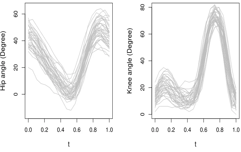
In this study, the goal is to understand how the joints in hip and knee interact during a gait cycle (Theologis, 2009), (Ramsay and Silverman, 2005). Here, there are longitudinal measurements of hip and knee angles taken on 39 children on 20 equispaced evaluation points inT = [0,1]. Figure 2.5 displays the observed individual trajectories of the hip and knee angles. The study of
0.0 0.2 0.4 0.6 0.8 1.0
0
20
40
60
t
Hip angle (Degree)
0.0 0.2 0.4 0.6 0.8 1.0
0
20
40
60
80
t
Knee angle (Degree)
Figure 2.5 Measurement of hip angles and knee angles in the gait study.
noise. Kim et al. (2018) investigated the effect of knee angles on hip angles and found the effect to be linear. In our functional linear concurrent modeling setup, we are therefore interested in testing H0 :β1(t) = 0 against the alternative H1 :β1(t) 6= 0, where β1(t) denotes the linear concurrent effect of hip angles on knee angles. We use our proposed testing method with 14 cubic B-splines to modelβ0(t) andβ1(t). The p-value of the proposed test is calculated to be
.0004. So we reject the null hypothesis and conclude that knee angle at any fixed time point is associated with the hip angle at the same time point. Our findings match with that of Kim et al. (2018), who used the bootstrapped-F test method.
As the sample size (n= 39) for this data is small and our testing method is an asymptotic one, we further evaluate the performance of our proposed method using a simulation study that captures the feature of the gait data. This also enables us to see the power performance of our method. This is done similarly as that of Kim et al. (2018). We use a model that mimics the feature of the gait data, generate a large simulated data set and assess the power performance of our method on the simulated data. In particular, We generate the covariate Xi(t) from a process with the mean and covariance functions that equal their estimated counterparts from the data using FPCA. We also estimate the parameters β0(t), β1(t) from the fit of our full model and estimate Σ(s, t) by doing FPCA on the residuals obtained from the full model fit. Then we generate observations using the model Yi(t) = ˆβ0(t) +d{Xˆi(t) ˆβ1(t)}+i(t), where
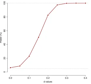
i(·)∼N(0,Σ(ˆ ·,·)). We simulaten = 300 response curves Yi(t) from the above set up. In the above set up d again plays the role of a parameter, which controls departure from the null hypothesis. We perform a power analysis simulating 1000 such data sets from the above scenario for variousd. Figure 2.6 shows the power curve obtained from our analysis.
d values
P
o
w
er (%)
0.0 0.1 0.2 0.3 0.4
0
20
40
60
80
100
Figure 2.6 Results from simulation study mimicking gait data. Displayed is the power curve of our
test.
2.4.2 Calcium Absorption Data
We consider the dietary calcium absorption study given in Davis (2002). In this study the subjects are a group of 188 patients. We have data on calcium absorption, dietary calcium intake and BMI of these patients at irregular intervals between 35 to 64 years of their ages. The number of repeated measurements for each patient is between 1 to 4. Figure 2.7 shows the individual curves of patients’ calcium absorption and calcium intake along their ages.
0.2 0.4 0.6
40 50 60
age
Calcium absor
ption
0.5 1.0 1.5 2.0
40 50 60
age
Calcium intak
e
Figure 2.7 Observed calcium absorption and calcium intake in the calcium absorption study.
are observed with measurement error. So our observed data is Ui(tij) = Xi1(tij) +δij and
Vi(tij) =Xi2(tij) +νij.
Our response variable is calcium absorptionYi(t). Following the study in Kim et al. (2018) we assume a functional linear concurrent regression model,Yi(t) =β0(t) +Xi1(t)β1(t) +Xi2(t)β2(t) +
i(t), and want to testH0:β2(t) = 0 against the alternative H1 :β2(t)6= 0.First we use FPCA as discussed in Section 2.2.5 on noisy covariates to get their smooth counterparts at time points where we have Yi(t) available and then apply our one sided score test method for multiple covariates described as in Section 2.2.6. We use 12 cubic B-Splines to model β0(t),β1(t) and
2.5
Discussion and Future Work
In this article, we have proposed a likelihood based method for testing of hypothesis in functional linear concurrent regression. We have formulated the problem as a test for variance component and have used a one sided score test approach. We have established the asymptotic null distribution of our test statistic under some standard assumptions. Through simulations, we have shown our proposed method maintains the nominal type I error rate and also yields higher power compared to the existing bootstrapped-F test, even when data is observed sparsely and with measurement error. We have successfully applied our method in finding significant covariates in two real data applications, namely the gait study and calcium absorption study. We note our method is a general one and can be applied for testing in longitudinal data setting too, where we have more flexibility in assuming a parametric form of error covariance structure and estimating it consistently from the data.
Software
Software in the form of R code illustrating implementation of the proposed method, together with the data set and complete documentation is available at GitHub (https://github.com/
rahulfrodo/FLCM_Score).
Acknowledgements
Chapter 3
Variable Selection in Functional
Linear Concurrent Regression
3.1
Introduction
et al., 2002, 2004), smoothing spline (Hastie and Tibshirani, 1993; Hoover et al., 1998; Chiang et al., 2001; Eubank et al., 2004) among many others. Similar to classical scalar regression, when there are a large number of covariates present, the primary interest might be to select only the set influential variables and estimate their effects. While doing significance testing and building confidence bands can help for assessing the individual effect of a predictor, they are computationally infeasible, when the number of covariates is large. Thus arises the need to perform variable selection in functional linear concurrent regression.
Our research in this article is motivated by a fisheries footprint study where the goal is to identify important time varying socio-structural and economic drivers influencing fisheries footprint (Global Footprint Network’s measure of total marine area required to produce the amount of seafood products a nation consumes) and to estimate their time varying effects. Although, a number of variable selection methods have been developed for scalar on function regression (Gertheiss et al., 2013; Fan et al., 2015) and function on scalar regression (Chen et al., 2016), literature for variable selection in functional linear concurrent regression is relatively sparse. Recently Goldsmith and Schwartz (2017) developed a variable selection method in functional linear concurrent model using a variational Bayes approach with sparsity being introduced through a spike and slab prior on the coefficients of the basis expansion of the regression functions. In this article we propose a variable selection method in functional linear concurrent regression extending the classically used variable selection methods like LASSO (Tibshirani, 1996) , SCAD (Fan and Li, 2001) and MCP (Zhang, 2010).
in which they use a group SCAD penalty for variable selection in varying coefficient models, but we propose a different penalty on the coefficient functions which simultaneously penalizes departure from sparsity as well as roughness of the coefficient functions, and our research shows there is much to be gained by using the group MCP penalty. A pre-whitening procedure similar to Chen et al. (2016) is employed to take into account temporal dependence present within functions. We also consider that the covariates might be contaminated with measurement error and therefore use functional principal component analysis (FPCA) to get denoised trajectories of the covariates which improves estimation accuracy of our approach. Through simulations, we illustrate our method, particularly with group SCAD or group MCP penalty, can pick out the relevant variables with very high accuracy and has minuscule false positive and false negative rate even when data is observed sparsely and is contaminated with measurement error. We demonstrate two real data applications of our method in the study of dietary calcium absorption (Davis, 2002) and the fisheries footprint study.
The rest of the article is organized as follows. In Section 3.2 we present our modeling framework and illustrate our variable selection method. In Section 3.3 we conduct a simulation study to evaluate the performance of our method and summarize the simulation results. In Section 3.4 we go back to the two real data examples; calcium absorption study and fisheries footprint study, apply our variable selection method to find out the influential covariates and present our findings. We conclude in Section 3.5 with a discussion about some limitations and possible extensions of our work.
3.2
Methodology
3.2.1 Modeling Framework and Variable Selection Method
for (i = 1,2, . . . , n), where Yi(·) is a functional response and Xi1(·),Xi2(·),. . . , Xip(·) are the corresponding functional covariates. We assume the covariates and the response are observed on a fine and regular grid of points S ={t1, t2, . . . , tm} ⊂S = [0, T] for some T > 0, and the covariates are measured without any error. We discuss later in this section how our model and method can be easily extended to accommodate more general scenarios where the covariates are contaminated with measurement error and observed sparsely. We consider a functional linear concurrent regression model of the form,
Yi(t) = p X j=1
Xij(t)βj(t) +i(t), (3.1)
whereβj(t) (j= 1,2, . . . , p) are smooth functions (finite second derivative) representing the func-tional regression parameters. We assumeXij(·) are independent and identically distributed (i.i.d.) copies ofXj(·) (j= 1,2, . . . , p), whereXj(·) s are underlying smooth stochastic processes. We fur-ther assumei(·) are i.i.d copies of(·), which is a mean zero stochastic process. The model (3.1) in stacked form can be rewritten asY(t) =X(t)β(t) +(t). Generally in functional linear concurrent regression, estimation is done (Ramsay and Silverman, 2005) by minimizing the penalized residual sum of square, SSE(β) =R
r(t)Tr(t)dt+Pp j=1λj
R
(Ljβj(t))2dt, wherer(t) =Y(t)−X(t)β(t). For example when Lj = I, we minimize
R
r(t)Tr(t)dt+Pp j=1λj
R
(βj(t))2dt. Now suppose {θkj(t), k= 1,2, . . . , kj} is a set of known basis functions forj= 1,2, . . . , p. We model the un-known coefficient functions using basis function expansion asβj(t) =Pkj
k=1bkjθkj(t) =θj(t)Tbj, whereθj(t) = [θ1j(t), θ2j(t), . . . , θKjj(t)]
T andb
j = (b1j, b2j, . . . , bkjj)
T is a vector of unknown coefficients. In this article, we use B-spline basis functions, however, other basis functions can be used as well. Then the minimization in the example mentioned above, can be carried out by min-imizingR
{Y(t)−X(t)Θ(t)b}T{Y(t)−X(t)Θ(t)b}dt+bT
Rb. Hereb, Θ(t) and penalty matrix R are defined in stacked form as b = (bT1,bT2, . . . ,bTp)T, Θ(t) = {θ1(t)T,θ2(t)T, . . . ,θp(t)T} and R=diag(R1,R2, . . . ,Rp), where Rj =λjbTj{
R
θj(t)θj(t)Tdt}bj. For our variable selection method we define penalty on the regression functions βj(·) as, Pλ,ψ{βj(·)} = λ[
R
ψR{βj00(t)}2dt]1/2 =λbT
jRjbj +ψbTjQjbj 1/2
=λ
bTjKψ,jbj 1/2
, where Kψ,j = Rj+ψQj, Rj ={R θj(t)θj(t)Tdt},Qj ={R θ
00
j(t)θ
00
j(t)Tdt}. This penalty was originally proposed by Meier et al. (2009) and later used by Gertheiss et al. (2013) for their variable selection method in scalar on function regression. The parameterψ≥0 controls the amount of penalization on the roughness penalty. The proposed penalty simultaneously penalizes departure from sparsity and roughness of the coefficient functions ensuring the resulting coefficient functions are smooth and small coefficient functions are shrunk to zero introducing sparsity. Subsequently, we propose to minimize the following penalized mean sum of square of the residuals for variable selection,
L(b) = 1/n
Z
{Y(t)−X(t)Θ(t)b}T{Y(t)−X(t)Θ(t)b}dt+λ p X j=1
(bTjKφ,jbj)1/2. (3.2)
Since we assume data is observed in a dense equispaced grid, the variable selection in practice is carried out by minimizing the following equivalent criterion,
n X i=1 m X l=1
[Yi(tl)− p X j=1
Xij(tl){ kj
X k=1
bkjθkj(tl)}]2+λmn p X j=1
(bTjKψ,jbj)1/2. (3.3)
Now using Cholesky decomposition of Kψ,j =Lψ,jLTψ,j and denotingγj =LTψ,jbj, the penalized sum of square of residuals can be reformulated as,
R(γ) = n X i=1 m X l=1
[Yi(tl)− p X j=1
Xij(tl){ kj
X k=1
bkjθkj(tl)}]2+λmn p X j=1
(bTjKψ,jbj)1/2
= n X i=1 m X l=1
[Yi(tl)− p X j=1
Z∗ij(tl)Tbj]2+λmn p X j=1
(bTjKψ,jbj)1/2, Z∗ij(tl)T =Xij(tl)×θj(tl)T
= n X i=1 m X l=1
[Yi(tl)− p X j=1 ˜ Zij ∗
(tl)Tγj]2+λmn p X j=1
(γjTγj)1/2, where Z˜ij
∗
(tl) =L−ψ,j1Z
∗
ij(tl)
= n X
i=1
||Yi−Z∗iγ||22+λmn p X j=1
(γjTγj)1/2 = n X
i=1 ||Yi−
p X j=1
Z∗ijγj|| 2
2+λmn p X j=1
(γjTγj)1/2,
Z∗i = ˜ Zi1 ∗
(t1)T Z˜i2
∗
(t1)T Z˜i3
∗
(t1)T . . . Z˜ip
∗
(t1)T ˜
Zi1
∗
(t2)T Z˜i2
∗
(t2)T Z˜i3
∗
(t2)T . . . Z˜ip
∗
(t2)T
. . . .
˜
Zi1
∗
(tm)T Z˜i2
∗
(tm)T Z˜i3
∗
(tm)T . . . Z˜ip
∗
(tm)T .
HereZ∗ij refers to the jth block column in this matrix. We recognize this minimization problem as performing a group LASSO (Yuan and Lin, 2006), where the grouping is introduced by covariates. In particular we obtain estimates of γj by minimizing similar penalized least square as in group LASSO namely;
ˆ
γ= argmin
γj,j=1,2,...,p
n X i=1
||Yi− p X j=1
Z∗ijγj|| 2
2+λmn p X j=1
(γjTγj)1/2
= argmin
γj,j=1,2,...,p
n X i=1
||Yi− p X j=1
Z∗ijγj||22+λmn p X j=1
||γj||2
= argmin
γj,,j=1,2,...,p
n X
i=1 ||Yi−
p X j=1
Z∗ijγj||22+mn p X j=1
PLASSO,λ(||γj||2). (3.4)
We extend this group LASSO formulation to non convex penalties, which are known (Breheny and Huang, 2015; Mazumder et al., 2011) to produce sparser and less biased estimates, especially when there are large number of variables and magnitude of original parameter of interest is large. In particular we propose to use two non convex penalties; SCAD (Fan and Li, 2001) and MCP (Zhang, 2010). These two penalties have been shown to ensure selection consistency and estimation consistency under standard assumptions in scalar regression case. They also enjoy the so called oracle property in which they behave like oracle MLE asymptotically. This motivates us to use them in our functional variable selection context, and then the problem of variable selection reduces to a group SCAD or group MCP problem in our modeling set up as follows.
Group SCAD Method
ˆ
γ= argmin
γj,j=1,2,...,p
n X
i=1 ||Yi−
p X j=1
Z∗ijγj|| 2 2+mn
p X j=1
PSCAD,λ,φ(||γj||2), (3.5)
where PSCAD,λ,φ(||γj||2) is defined in the following way:
PSCAD,λ,φ(||γj||2) =
λ||γj||2 if||γj||2≤λ.
λφ||γj||2−.5(||γj||22+λ2)
φ−1 ifλ <||γj||2≤λφ.
.5λ2(φ+ 1) if||γj||2> λφ.
Group MCP Method
For Group MCP method estimation of γ is done similarly,
ˆ
γ= argmin
γj,j=1,2,...,p
n X
i=1 ||Yi−
p X j=1
Z∗ijγj||22+mn p X j=1
PM CP,λ,φ(||γj||2), (3.6)
where PM CP,λ,φ(||γj||2) is defined as,
PM CP,λ,φ(||γj||2) =
λ||γj||2−||γj|| 2 2
2φ if||γj||2 ≤λφ.
.5λ2φ if||γ
j||2 > λφ.
3.2.2 Incorporating Covariance Structure into variable selection
covariance kernelG(s, t) andwt is a white noise with varianceσ2. The covariance function of the error process is then given by Σ(s, t) = cov{(s), (t)} = G(s, t) +σ2I(s = t). For data observed on dense and regular grid the covariance matrix of the residual vector is the given by Σ=diag{Σm×m,Σm×m, . . . ,Σm×m}, whereΣm×mdenotes the covariance kernel Σ(s, t) evaluated at S = {t1, t2, . . . , tm}. Now if Σm×m is known, redefining Yi and Z∗ij as Yi = {Σ
−1/2 m×m}Yi, Z∗ij ={Σ
−1/2 m×m}Z
∗j
i , the same penalized criterion (4), (5) or (6) can be used to perform variable selection.
In reality Σ is unknown, and we need an estimator ˆΣ. In the context of functional data, we want to estimate Σ(·,·) nonparametrically. If we had the original residualsij available, we could use functional principal component analysis (FPCA), e.g., Yao et al. (2005) or Zhang et al. (2007) to estimate Σ(s, t). If the covariance kernelG(s, t) of the smooth partV(t) is a Mercer
kernel (Mercer, 1909), by Mercer’s theorem G(s, t) must have a spectral decomposition
G(s, t) =
∞
X k=1
λkφk(s)φk(t),
whereλ1 ≥λ2≥. . .0 are the ordered eigenvalues andφk(·)s are the corresponding eigenfunctions. Thus we have the decomposition Σ(s, t) = P∞
k=1λkφk(s)φk(t) +σ2I(s = t). Given tij =
V(tij) +wij, one could employ FPCA based methods to get ˆφk(·), ˆλks and ˆσ2. So an estimator of Σ(s, t) can be formed as ˆΣ(s, t) =PK
k=1λˆkφˆk(s) ˆφk(t) + ˆσ2I(s=t),whereK is large enough for the convergence to hold and is typically chosen such that percent of variance explained (PVE) by the selected eigencomponents exceeds some pre-specified value such as 99% or 95%.
In reality we don’t have the original residuals ij and use the full model (1) to obtain residuals
eij =Yi(tj)−Yˆi(tj). Then treatingeij as our original residuals, we obtain ˆΣ(s, t) using FPCA.
equivalent linear model of criterion (4), (5) or (6) and this has shown good performance in our simulation study. Chen and Chen (2008) established consistency of EBIC under standard assumptions and illustrated its superiority over other methods like cross-validation, AIC, and BIC, which tend to over select the variables. For tuning parameter φwe use the values 4 for SCAD and 3 for MCP, as proposed by the original authors. For model fitting we use ‘grpreg’ package (Breheny, 2019) in R.
Remark 2: In practice, we recommend standardizing the variables either using Euclidean norm (automatically performed in ‘grpreg’) or using FPCA based methods (Xj∗(t) = Xj(t)−µj(t)
σj(t) ),
which is especially useful for highly sparse data where some B-splines might not have observed data on its support. This can help in faster convergence of the proposed method. We performed both the standardization methods in our simulation studies and obtained very similar results.
3.2.3 Extension to Sparse data and Noisy Covariates
More generally, we can consider the case where data is observed sparsely and covariates are observed with measurement error. This is most often the case for longitudinal data. Here the observed data is the response {(Yi(tij), tij), j = 1,2, . . . , mi} and the observed covariates {(U1(t1ij), t1ij), j = 1,2, . . . , m1i}, {(U2(t2ij), t2ij), j = 1,2, . . . , m2i},. . . ,{(Up(tpij), tpij), j = 1,2, . . . , mpi}. Let us denoteUk(tkij)s, (k = 1,2,3, . . . , p) by Uijk . Here Uijk s represent the observed covariates with measurement error, i.e., we haveUijk =Xk(tkij)+eijkfori= 1,2, . . . , n,
j = 1,2, . . . , mki and k = 1,2, . . . , p. The measurement error eijk are assumed to be white noises with zero mean and variance σk2. In sparse data set up it is generally assumed (Kim et al., 2018) although individual number of observations mi is small, Sni=1
Smi
PACE method as in Yao et al. (2005). Then these estimates are put together using Karhunen-Lo`eve expansion (Karhunen, Loeve 1946) to get estimates ˆXik(·) of the true curves Xik(·) as ˆXik(t) = ˆµk(t) +
PS
s=1ζˆiskψˆsk(t), where the number of eigenfunctions S to use is chosen using the percent of variance explained (PVE) criterion, which is the percentage of variance explained by the first few eigencomponents. Alternatively one can also use multivariate FPCA (Happ and Greven, 2018) instead of running FPCA on each predictor variable separately. Then for sparse data observed on irregular grid and observed with measurement error, we use {Yi(tij),Xˆi1(tij),Xˆi2(tij), . . . ,Xˆip(tij)j= 1,2, . . . , mi}ni=1 as our original data and use this data for performing variable selection.
3.3
Simulation Study
3.3.1 Simulation Set Up
In this section, we evaluate the performance of our variable selection method using a simulation study. To this end we generate data from the model,
Yi(t) =β0(t) + 20 X j=1
Xij(t)βj(t) +i(t) i= 1,2, . . . , n, t∈[0,100].
The regression functions representing the dynamic effects are given by β0(t) = 8sin(πt/50),
β1(t) = 5sin(πt/100),β2(t) = 4sin(πt/50)+4cos(πt/50),β3(t) = 25e−t/20and rest of theβj(t) = 0 forj= 4,5,6, . . . ,20, i.e., the last 17 covariates are not relevant. The original covariatesXij(·)iid∼
Xj(·), whereXj(t) (j= 1,2, . . . ,20) are given byXj(t) =aj √
2sin(πjt/400)+bj √
2cos(πjt/400), where aj ∼ N(50,(2)2), bj ∼ N(50,(2)2). We moreover assume that Xij(t) are observed with measurement error i.e., we observeUij(t) =Xij(t) +δj, whereδj ∼ N(0, .62). The error process
i(t) is generated as follows;
where ξi1 iid∼ N(0, .52) andξi2 iid∼ N(0,0.752). The response Yi(t) and noisy covariateUij(t)’s are observed sparsely in randommi points inS, whereSis the set ofm= 81 equidistant time points in [0,100] andmi
iid
∼ U nif orm{30,31, . . . ,41}. Three sets of sample size n∈ {100,200,400} are considered. For each sample size, we use 500 replicated datasets for evaluation of our method.
3.3.2 Simulation Results
Our primary interest is selection (identification) of the relevant covariates X1(·), X2(·), X3(·) and estimating their effects β1(t), β2(t), β3(t) accurately. As the covariates are observed sparsely and with measurement error, we apply FPCA as discussed in Section 3.2.3 with PVE = 99% and obtain the denoised curves ˆXij(t) before applying our variable selection method. We apply the proposed variable selection method with and without the pre whitening procedure mentioned in Section 3.2.2. Table 3.1 and Table 3.2 display the selection percentage of each variable for each of the three selection methods discussed in Section 3.2 and for the three sample sizes
to the true model size 3 (exactly 3 with pre whitening procedure in Table 3.2). These results also illustrate the benefit of pre-whitening and henceforth we have used pre-whitening as a pre processing step to perform variable selection using the proposed methods.
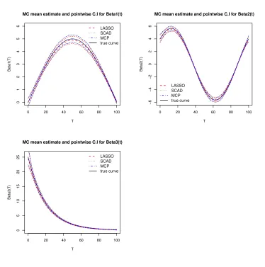
Next, as an assessment of the accuracy of the estimates ˆβk(t) (k= 1,2,3), we plot the true regression curves overlaid by their Monte Carlo (MC) mean estimate. MC point-wise confidence intervals (95%) (corresponding to 2.5 and 97.5 percentile) for each of the three curves are also plotted to asses variability of the estimates. Figure 3.1 displays this plot forn= 200, the plots forn= 100, n= 400 are similar with more accuracy and less variability for larger sample sizes.
0 20 40 60 80 100
0
1
2
3
4
5
6
MC mean estimate and pointwise C.I for Beta1(t)
T
Beta1(T)
LASSO SCAD MCP true curve
0 20 40 60 80 100
−6
−4
−2
0
2
4
6
MC mean estimate and pointwise C.I for Beta2(t)
T
Beta2(T)
LASSO SCAD MCP true curve
0 20 40 60 80 100
0
5
10
15
20
25
MC mean estimate and pointwise C.I for Beta3(t)
T
Beta3(T)
LASSO SCAD MCP true curve