Tree-Structured Neural Decoding
Christian d’Avignon [email protected]
Department of Biomedical Engineering Johns Hopkins University School of Medicine 720 Rutland Avenue, Traylor Building 608 Baltimore, MD 21205, USA
Donald Geman [email protected]
Department of Mathematical Sciences and Whitaker Biomedical Engineering Institute Johns Hopkins University
3400 N. Charles Street, Clark Hall 302A Baltimore, MD 21218, USA
Editor: Peter Dayan
Abstract
We propose adaptive testing as a general mechanism for extracting information about stimuli from spike trains. Each test or question corresponds to choosing a neuron and a time interval and check-ing for a given number of spikes. No assumptions are made about the distribution of spikes or any other aspect of neural encoding. The chosen questions are those which most reduce the uncertainty about the stimulus, as measured by entropy and estimated from stimulus-response data. Our exper-iments are based on accurate simulations of responses to pure tones in the auditory nerve and are meant to illustrate the ideas rather than investigate the auditory system. The results cohere nicely with well-understood encoding of amplitude and frequency in the auditory nerve, suggesting that adaptive testing might provide a powerful tool for investigating complex and poorly understood neural structures.
Keywords: Adaptive Testing, Decision Trees, Neural Decoding.
1. Introduction
Applications of machine learning to pattern recognition often involve converting sensory data to semantic descriptors, as in recognizing objects in natural images and words in natural speech. Generally performance is measured by classification accuracy. We propose a somewhat different scenario—an application of machine learning to neuroscience in which the principal objective is to discover information about the encoding of sensory stimuli in actual neurons. Specifically, we construct decision trees to classify simple sounds based on auditory spike train data in order to explore the encoding process itself. If the types of queries selected during learning are revealing, then sequential adaptive testing might provide a powerful tool for exploratory neuroscience, e.g., hypothesis generation.
shall adopt the “point of view of the organism” (Rieke et al., 1999): How might a figurative being, situated within the brain and observing only neural spikes, interpret incoming but unseen stimuli, in fact provide a “running commentary” about the stimuli, based only on simple functions of the sequence of spikes?
We attempt to classify stimuli based on patterns of spike time occurrences rather than, say, “firing rates.” Interest is this direction, whereas relatively new, is rapidly growing (see Hopfield, 1995, for example). Also, the general idea of classifying spike trains has gained further appeal due to the development of certain families of metrics for comparing sequences of spikes (Victor and Purpura, 1997; Victor, 2000). However, our approach is markedly different from these, and, as far as we know, entirely novel.
Specifically, we consider the possibility of decoding instructions in the form of a tree of binary questions somehow implemented in the brain. One motivation is that decisions in the nervous sys-tem are made through interactions of spikes from different neurons on a particular target neuron. The effect on the target neuron of a spike is short-term and lasts for a period of time up to the time constant of the target, typically 10 ms or so. Thus it makes sense for the present work to consider questions of the form “Did a spike occur in a particular short time interval?” In addition, it is clear that the synchronous occurrence of spikes in multiple inputs to a neuron is an important event in many situations (Koch, 1999). Thus we seek a form of question that can easily incorporate infor-mation about simultaneous, or nearly simultaneous, patterning of events across multiple neurons.
An overview of the decoding strategy—how the spike trains are processed and the stimulus is estimated—is presented in the following section, where some related work is mentioned. Whereas our queries are not the standard ones based on a “feature vector,” this section is intended primarily for readers unfamiliar with decision trees and their induction from training data. The stimulus and response variables are defined in Section 3 and tree induction is summarized in Section 4, assuming a background in machine learning. These two sections are more technical. In Section 5 we present experiments on amplitude and frequency decoding, with particular attention to the nature of the selected questions and coherence with knowledge of the auditory system. The results are further analyzed in Section 6 with respect to improvements and extensions, for instance how the method might be used to investigate more complex systems. Finally, our main conclusions are summarized in Section 7.
2. Overview of the Method
The particular questions we consider are based on the presence or absence of spikes in selected time intervals of the recent past. No assumptions are made about the encoding process. Relative to a fixed set of time intervals and family of neurons, each question is of the form: “For neuron
The building blocks for our pool of questions—time intervals, choice of neuron and number of spike occurrences—are of course natural objects of study in neural coding. Indeed, the importance of the precise timing of spikes emerges from many different experiments and theoretical investiga-tions (Victor, 2000; Wiener and Richmond, 2001; Panzeri et al., 2001). In addition, both a proper accounting of which neuron is responsible for which spike (Reich et al., 2001; Frank et al., 2000) and the correlations among spikes (Nirenberg and Latham, 2003; Panzeri and Schultz, 2001) are considered important to understanding neural decoding. In our framework, such correlations are captured through the conjunction of answers to multiple questions.
The selection of questions, i.e., the actual construction of the decision tree, is based on entropy reduction: At each stage choose the question which most reduces the conditional entropy of the “class variable”—in our case the stimulus—given the new question and the previous answers; see Section 4. Mean entropies and answer statistics are estimated from data by standard inductive learning (Breiman et al., 1999). In our case, spike train data generated by simulating the conduction of auditory nerve responses to pure tones. Although we do not consider transient stimuli, we attempt to estimate the stimulus based only on observing spikes in the recent past.
Informally, we begin at the root of the tree with all the elements of the training set. Based on entropy considerations, we then find that question from our pool which most decisively splits the elements residing at the root node into two subsets, one residing at the “no” child node and the other at the “yes” child. The same splitting procedure is then applied to these two nodes, and the construction proceeds recursively until a stopping criterion is met, at which point the stimulus is estimated by the most common value of the remaining data elements.
Sequences of yes/no questions directly about the identity of the stimulus are considered by Nirenberg and Latham (2003) in order to measure the loss in efficiency in assuming independence among neurons; the strategies there are the ideal ones that characterize optimal codes (reach the theoretical entropy bound) rather than those found here (and in machine learning), namely decision trees induced from data using questions which are realizable as features of the observations (spike trains).
A quantitative description of the experimental scenario and tree construction follows in the next two sections.
3. The Stimulus-Response Scenario
The stimuli are pure tones and hence characterized by an amplitude , a frequency and a phase , restricted to intervals , and , respectively. Amplitude corresponds to loudness and can be expressed in decibels (dB); frequency corresponds to the pitch and is expressed in Hertz (Hz); phase could be expressed in radians. For human hearing, we might take 10 dB 60 dB ,
16 Hz 16 kHz and 0 2 . Phase is an important neurophysiological cue, and particularly crucial for sound localization; however, since it is processed at stages ulterior to the auditory nerve, we set it to zero and therefore consider zero-phase sinusoidal acoustic waves with time-independent amplitude and frequency. The set of possible stimuli is then sin t : t I0 , where I0is a time interval.
The set of possible single-neuron responses, namely finite sequences of spike times, is
ti i 1 . In order to emphasize the “running commentary,” the spikes are investigated on the
the corresponding time buffer and shall be understood as the present—the instant at which the figurative being generates the current commentary.
Let S R N be a stimulus-response pair. Note that R is a collection of N spike trains and that S and R are regarded as random variables whose joint distribution is of course unknown. As usual, the training set is an i.i.d. sample from S R . Since the stimulus is determined by and
, the training set, say of size J, is denoted by
1 1 r1 J J rJ
4. The Tree-Structured Decoder
Suppose the continuous parameter space is quantized into rectangular bins corresponding to partitioning amplitude and frequency: Ku 1 uand Kv 1 v, where all components are
intervals. In effect, we discretize to K K values, which can be thought of as the centers of
rectangular bins uv 1 u K 1 v K . In practice, stimuli are selected by randomly choosing
samples from each bin.
The decoder is constructed by decision tree induction using stepwise uncertainty reduction. Since both the “feature vector” (R) and the “class labels” (S) are nonstandard, we need to specify the set of “questions” (splitting rules) and how conditional entropy (the splitting criterion) is estimated for each possible question.
The questions are determined by checking for a particular number of spikes in a particular time interval for a particular neuron. More formally, denote by R R 1 R N the responses of the
N neurons. There is a binary question, XnAm R , for each neuron n, each subinterval A c
and each non-negative integer m representing a spike count:
XnAm R 1 if R n A m;
0 otherwise
Of course we cannot consider all such questions as actual candidates and if the number we do consider is very large there is sure to be overfitting. Hence we restrict the intervals to
L
l 1
j 1
l c
j
l c : j 0 l 1
for certain values of L and write X for the resulting set of questions:
X XnAm R : A n 1 N m 0 M
For example, if L 3 and c 60 ms, then
0 60 0 30 30 60 0 20 20 40 40 60
and if n m 2, then each question in X identifies one of two neurons, an interval I and asks whether that neuron exhibited zero, one or two spikes in I. We could imagine other families, such as only intervals of the form t or c t for certain c t , but for simplicity we restrict
our discussion to X .
of R, the tree T is also regarded as a random variable taking values in the set of leaves and every training example i i r i traverses a unique path down the tree determined only by ri . Let
B denote the event that node is reached and let be the set of training examples arriving at . The estimated distribution of the (quantized) stimulus at node is
ˆ
p u v 1
i 1
1 si ri 1 si
uv u 1 K v 1 K
where S S S . The uncertainty in the stimulus at is characterized by the condi-tional entropy H S B , estimated by H ˆp and the test X at node is the one minimizing the empirical estimate of H S B X .
Finally, a node is designated terminal—a leaf—if either i) 10, thus avoiding small-sample estimates (see the discussion in Paninski, 2003), or ii) the entropy H ˆp falls below a threshold (see Section 5) which is chosen so that the estimated stimulus distribution is appropriately concentrated.
5. Experimental Results
To demonstrate the decoding algorithm, we consider spike trains traveling through the auditory nerve, a bundle of about 30,000 neurons in the inner ear which originates from the basilar membrane situated in the cochlea. Auditory nerve fibers have an inherent frequency selectivity so that each fiber is most sensitive to its particular best frequency, with monotonically declining sensitivity to adjacent frequencies. Fibers also increase their rate of firing of action potentials as the amplitude of the stimulus increases; however, each fiber has a limited dynamic range so that the discharge rate saturates at some stimulus amplitude. In order to better appreciate the experiments, the interested reader might consult a standard neuroscience source (Kandel et al., 2000) or an introductory text on the auditory system (Pickles, 1988).
The spike train data are not obtained from actual neurons, but rather from a model (Heinz et al., 2001) whose realizations are nearly indistinguishable from the responses to pure tones of real neurons in the auditory nerve. Spike trains are generated for single fibers and for small populations of fibers, chosen to have best frequencies distributed across the auditory frequency range, and binary decision trees are then induced as described in Section 4.
Ideally, the trees would have very low-entropy leaves—in other words, leaves for which ˆp
is peaked around some parameter bin, which then serves as our estimate of the stimulus. However, we do not attempt to enforce very strong peaking, as in most classification studies, for instance choosing an entropy threshold less than unity. Instead, our stopping criterion is H ˆp 1 25. To understand this choice, and how this parameter might be adjusted for other purposes, recall that a distribution concentrated on two values has entropy at most H log22 1 (two equal masses); also, the entropies of the distributions 3 4 1 8 1 8 and 1 2 1 4 1 4 are, respectively, H 1 06 and
H 1 5. As a result, if H ˆp 1 25 and if the estimated leaf distribution ˆp is accurate, then our
estimate of the stimulus is likely to be roughly correct, which is all we are demanding in the context of this paper.
about this process based on analyzing the nature of the questions which yield the most accurate estimates of the stimulus.
5.1 Amplitude Decoding
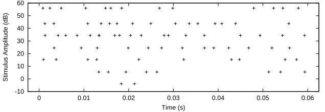
We begin by investigating a single-neuron, randomly chosen and subjected to varying amplitudes at the neuron’s best frequency. Specifically, we take 2 kHz and 5u 1 uwhere u
10u 10u 10 . There are then seven classes. The stimuli in the training set are 100 amplitudes randomly selected from each of the seven bins u1, 1 u 7 (therefore 700) and the
cor-responding responses are then simulated for the given neuron. Figure 1 shows one spike train per amplitude.
-10 0 10 20 30 40 50 60
0 0.01 0.02 0.03 0.04 0.05 0.06
Stimulus Amplitude (dB)
Time (s)
Figure 1: Spike trains of a single neuron in response to sinusoidal stimuli at frequency 2 kHz and seven different amplitudes.
The time interval is Ic I0 0 0 06 . A tree was constructed with maximal depth D 10 and questions based on the parameters M 5 and L 20, meaning we can check for exactly 0–5 spikes in intervals of 20 different sizes. In fact, nine different trees were constructed from nine training sets and statistics for each tree were collected based on independent test sets. Aggregate statistics refer to averaging over the nine experiments. The mean tree depth is 7 68 and mean leaf entropy is 1 63 (as compared with 1 13 with the training data), computed from empirical estimates of the probability of reaching each leaf. As a classifier of the amplitude, the performance is about the same for training and test data, namely about 77% of the time the estimated amplitude bin is within one of the true one.
Figure 2 shows the distribution of the questions chosen in terms of the interval length, l, and the number of spikes, m, where the averaging is with respect to the (normalized) probabilities of reaching internal nodes. Again, all results are averaged over repeated experiments. (The results for a single tree are approximately the same.) Clearly, a wide range of interval sizes are selected, ranging from 3–60 ms. In contrast, there is a marked preference for checking for either at least one spike (m 0) or exactly one spike (m 1).
To appreciate what the trees are doing—what spike information is sought—consider the first questions. At the root, the amplitude count vector is 100 100 100 100 100 100 100 , and the corresponding distribution has entropy log27 2 81. The first question is “Is there at least one
spike during time interval [0,0.0033]?”. The “yes” child has counts 9 16 32 72 93 99 100 and
the “no” child has counts 91 84 68 28 7 1 0 . The question at the “no” child is “Is there at least
0 0.05 0.1
5 10 15 20
Frequency
Length Index
0 0.25 0.5
0 1 2 3 4 5
Frequency
Type Index
Figure 2: Frequency distributions for interval length (l) and numbers of spikes (m) for single-neuron amplitude decoding, averaged over nine trees.
28 40 63 28 7 1 0 and 63 44 5 0 0 0 0 , respectively. This last node is a leaf under our stop-ping criterion. One can observe a tendency to check shorter intervals in the half-tree with leaves identified with higher amplitudes and longer intervals in the other half-tree. Shorter intervals, of course, are more likely to contain a spike at the higher discharge rates produced by higher intensi-ties. The intervals at the onset of the stimulus are the most informative, and therefore are chosen for the early questions, because the discharge rate is highest at stimulus onset due to the rate-adaptation property of auditory neurons.
We reduced the number of possible questions by considering only L 10 interval sizes and checking only for the presence of at least one spike (i.e., M 0). Figure 3(a) provides an empirical justification for this reduction by comparing the mean node entropy by tree depth (for the first five levels) using both training data and test data for the two sets of parameters. (Setting L 20 and
M 5 yields 1260 possible questions per spike train, whereas setting L 10 and M 0 yields only 55.) The entropy drops clearly demonstrate that there is substantial overfitting in the case of the larger set of questions, as training data entropy drops are much larger than with test data. This is not the case for the smaller set of questions, and from here on all experiments use this reduced set
of questions.
Figure 3(b) gives the resulting distribution of lengths for single-neuron amplitude decoding with the reduced set of questions (for which training estimates are less biased); again there is a more or less uniform length usage. The corresponding mean tree depth and mean terminal entropy are 7 48 and 1 56, respectively, and the “within-one-bin” classification rate is 77%.
Consider now multiple neurons. We kept the same fixed frequency but randomly chose 15 neurons spread out along the basilar membrane. Thus, 700 but each ri is a vector of 15 spike trains. This time we reduced the time interval Ic during which queries take place to Ic 0 0 01
since, in the previous experiment, the chosen intervals usually started at or close to 0.
1.4 1.6 1.8 2 2.2 2.4 2.6 2.8
1 2 3 4 5
Mean Node Entropy (bits)
Level (a)
(i) (ii) (iii) (iv)
0 0.1 0.2
2 4 6 8 10
Frequency
Length Index (b)
Figure 3: (a) Mean node entropies by depth for 60 ms buffer and large set of questions with (i) training data and (ii) test data and for 10 ms buffer and small set of questions with (iii) training data and (iv) test data; (b) Frequency distribution for interval length (l) for single-neuron amplitude decoding, averaged over nine trees.
0 0.15 0.3
2 4 6 8 10
Frequency
Length Index (a)
0 0.3 0.6
3 6 9 12 15
Frequency
Neuron Index (b)
Figure 4: Frequency distributions for interval length (l) and chosen neuron (n) for multi-neuron amplitude decoding.
leads to spurious entropy drops due to overfitting rather than decoding. Of course, the reason why neurons tuned to frequencies away from the stimulus frequency are less informative here may be due to the relatively low sound levels (up to 60 dB) used. At higher sound levels, the response is expected to spread considerably along the frequency axis and off-stimulus frequency fibers are expected to be more important in intensity coding (Siebert, 1968).
5.2 Frequency Decoding
Whereas the mean tree depth is above 9 and the initial (root) entropy is log215 3 91, the mean terminal entropy is still above 3, meaning that the optimal questions yielded insignificant reductions in uncertainty about the frequency. However, this result is in fact consistent with tonotopic encoding,
wherein each neuron represents frequencies near its own best frequency. Frequency decoding with
a single neuron is only possible with a narrow range of frequencies near the neuron’s best frequency.
0 2 4 6 8 10 12 14 16
0 0.01 0.02 0.03 0.04 0.05 0.06
Neuron
Time (s)
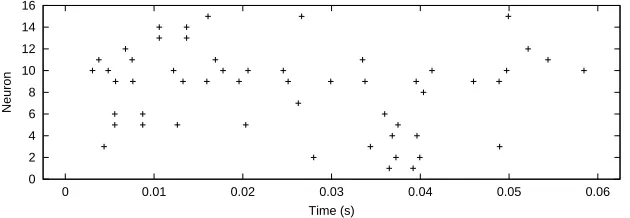
Figure 5: Spike train responses from 15 neurons to a sinusoidal stimulus with amplitude 30 dB and frequency 1 066 kHz.
For multiple neurons, we sampled 15 neurons in the auditory nerve uniformly along the basilar membrane. Otherwise, the protocol is the same as before, there again being 15 frequency bins. Figure 5 shows examples of spike trains for the fifteen neurons at one of the frequencies. The mean tree depth is now 8 62 and the mean terminal entropy is 2 03 (1 6 with training data). Thus, in comparison with a single neuron, this tree is slightly less deep and considerably more powerful; the classification rate is 63% to within one bin. Extending the sampled neurons from a single one to 15 along the basilar membrane thus enables decoding of frequency. This suggests (correctly)
that information about frequency is therefore carried by a set of neurons, in contrast to amplitude information, which (as seen before) is carried by any of the neurons.
6. Discussion
Decision trees are a standard tool in machine learning for inducing classifiers from data. Typically the goal is to predict the label of an unseen example, often in cases which are trivial for human sensory processing, for example recognizing handwritten digits or detecting faces in digital images. Very high accuracy is desired. Our context is different: The measurements are spike trains, the “class labels” refer to properties of a time-varying stimulus, and, perhaps most importantly, the primary concern is to determine what the decoding process reveals about which aspects of the stimulus are encoded by particular neurons and how this is achieved.
neu-ron is far from sufficient, whereas enough information to crudely predict the given frequency can be gathered from around eight questions from neurons distributed along the basilar membrane. In both cases, this makes sense biologically—inferring that information about the amplitude is included in each neuron is indeed correct, as is the insufficiency of a single neuron for frequency decoding.
On the other hand, how such mechanisms might arise in real brains is unclear, as is the mech-anism for sequential learning—how all this might be done efficiently as information accumulates, whether in natural or artificial systems. In the case of trees, it remains to determine the updating or deepening process, for instance how inefficient questions might be replaced without starting over from scratch.
In the spirit of developing a generic tool for investigating neural decoding, we have not assumed any specific mathematical model (Barbieri et al., 2001; Frank et al., 2000; Wiener and Richmond, 2001; Dimitrov and Miller, 2001). Moreover, we have avoided incorporating specific prior knowl-edge of the physiological properties of the structure under study, in our case auditory neurons. For instance, due to the wide spectrum of allowed intensities, many neurons are in a saturation mode, and thus do not carry information about intensity variations. Moreover, the simulated data is based on neurons randomly positioned along the basilar membrane; on average, they cover the length but are not (logarithmically) uniformly spaced in any given experiment. Constraints on the intensity range and spacing along the membrane would likely increase the performance of the classifier, but at the expense of limiting the applicability of the method. The types of assumptions we make are about the available questions; and the parameters involve choices in the tree-construction protocol, such as how many questions to ask before attempting estimation of the stimulus.
It would likely not be difficult to increase the decoding accuracy even without incorporating specific prior knowledge. For one thing, the parameters have not been tuned. For another, more questions, and/or more powerful questions, could be considered without promoting overfitting by a variety of well-known methods, such as randomization (Amit and Geman, 1997). In particular, it would be interesting to entertain questions which simultaneously query two or more neurons, for example checking for conjunctions of events in two spike trains, such as the joint occurrence of a spike in intervals in two different spike trains. In addition, recalling that the brain can function in a massively parallel fashion, one might produce multiple trees (e.g., using randomization or boosting) for querying the same spike trains; combining them in now standard ways would likely significantly increase the accuracy relative to individual trees. Finally, we considered only very small time buffers, whereas organisms greatly improve performance by integrating information over much longer time periods. For example, our procedure might be implemented every 10 ms and new decisions, and change detection, might be based on “recent” estimates as well as fresh explorations of the spike trains, especially when strong coherence is observed. This would be somewhat akin to the added information of video relative to still images.
7. Conclusion
The encoding of the amplitude and frequency of pure tones in auditory nerve spike trains is a well-understood process. It was hoped that information provided independently from tree-structured decoding would cohere with known results. This seems to have been the case: When the stimulus was well-classified by adaptive testing, the questions did indeed make sense biologically, whereas in those cases in which performance was poor there was also a biological interpretation (for example attempting frequency decoding with a single neuron). The results are therefore encouraging.
As to future work, besides extending this framework to synchronized questions and generating a “running commentary,” as discussed earlier, one could examine more complex stimuli at the level of the auditory nerve, such as tones varying jointly in amplitude and frequency, or examine responses in higher auditory structures such as the cochlear nucleus or the inferior colliculus. More generally, having tested the method on a well understood benchmark system, one can now envisage applying it to other systems of interest to the neurophysiology community, and thereby contribute to evaluating standing hypotheses or generating new ones.
Acknowledgments
We wish to thank Dr. Eric D. Young from the Neural Encoding Laboratory at the Johns Hopkins University School of Medicine for his valuable advice throughout this project. This project was supported in part by ONR under contract N000120210053, ARO under grant DAAD19-02-1-0337 and NSF ITR DMS-0219016. In addition, we are grateful to the referees for aiding us in relating this work to the literature in neuroscience.
References
Y. Amit and D. Geman. Shape quantization and recognition with randomized trees. Neural
Com-putation, 9:1545–1588, 1997.
R. Barbieri, M. Quirk, L.M. Frank, M.A. Wilson, and E.N. Brown. Construction and analysis of non-poisson stimulus response models of neural spike train activity. J. Neurosci. Meth., 105: 25–37, 2001.
L. Breiman, J.H. Friedman, R.A. Olshen, and C.J. Stone. Classification and Regression Trees. CRC Press, New York, 1999.
A.G. Dimitrov and J.P. Miller. Neural coding and decoding: communication channels and quanti-zation. Network: Comput. Neural Syst., 12:441–472, 2001.
L.M. Frank, E.N. Brown, and M.A. Wilson. Trajectory encoding in the hippocampus and entorhinal cortex. Neuron, 27:169–178, 2000.
M.G. Heinz, X. Zhang, I.C. Bruce, and L.H. Carney. Auditory nerve model for predicting perfor-mance limits of normal and impaired listeners. ARLO, 2:91–96, 2001.
E.R. Kandel, J.H. Schwartz, and T.M. Jessell. Principles of Neural Science 4th Edition. Appleton and Lange, New York, 2000.
C. Koch. Biophysics of Computation: Information Processing in Single Neurons. Oxford University Press, New York, 1999.
S. Nirenberg and P.E. Latham. Decoding neuronal spike trains: How important are correlations.
PNAS, 100(12):7348–7353, 2003.
L. Paninski. Estimation of entropy and mutual information. Neural Computation, 15:1191–1253, 2003.
S. Panzeri, R. Petersen, S. Schultz, M. Lebedev, and M.E. Diamond. The role of spike timing in the coding of stimulus location in rat somatosensory cortex. Neuron, 29:769–777, 2001.
S. Panzeri and S.R. Schultz. A unified approach to the study of temporal, correlational, and rate coding. Neural Computation, 13:1311–1349, 2001.
J.O. Pickles. An Introduction to the Physiology of Hearing 2nd Edition. Academic Press, London, 1988.
D.S. Reich, F. Mechler, and J.D. Victor. Independent and redundant information in nearby cortical neurons. Science, 294:2566–2568, 2001.
F. Rieke, D. Warland, R. de Ruyter van Steveninck, and W. Bialek. Spikes: Exploring the Neural
Code. MIT Press, Cambridge, MA, 1999.
W.M. Siebert. Stimulus transformation in the peripheral auditory system. In P.A. Kolwers and M. Eden, editors, Recognizing Patterns, pages 104–133, Cambridge, MA, 1968. MIT Press.
J.D. Victor. How the brain uses time to represent and process visual information. Brain Research, 886:33–46, 2000.
J.D. Victor and K.P. Purpura. Metric-space analysis of spike trains: theory, algorithms and applica-tion. Network: Comput. Neural Syst., 8:127–164, 1997.