Tree Induction vs. Logistic Regression: A Learning-Curve Analysis
Claudia Perlich [email protected]
Foster Provost [email protected]
Jeffrey S. Simonoff [email protected]
Leonard N. Stern School of Business New York University
44 West 4th Street New York, NY 10012
Editor: William Cohen
Abstract
Tree induction and logistic regression are two standard, off-the-shelf methods for building models for classification. We present a large-scale experimental comparison of logistic regression and tree induction, assessing classification accuracy and the quality of rankings based on class-membership probabilities. We use a learning-curve analysis to examine the relationship of these measures to the size of the training set. The results of the study show several things. (1) Contrary to some prior observations, logistic regression does not generally outperform tree induction. (2) More specifically, and not surprisingly, logistic regression is better for smaller training sets and tree induction for larger data sets. Importantly, this often holds for training sets drawn from the same domain (that is, the learning curves cross), so conclusions about induction-algorithm superiority on a given domain must be based on an analysis of the learning curves. (3) Contrary to conventional wisdom, tree induction is effective at producing probability-based rankings, although apparently comparatively less so for a given training-set size than at making classifications. Finally, (4) the domains on which tree induction and logistic regression are ultimately preferable can be character-ized surprisingly well by a simple measure of the separability of signal from noise.
Keywords: decision trees, learning curves, logistic regression, ROC analysis, tree induction
1. Introduction
In this paper1 we compare two popular approaches for learning binary classification models. We combine a large-scale experimental comparison with an examination of learning curves2to assess the algorithms’ relative performance. The average data-set size is larger than is usual in machine-learning research, and we see behavioral characteristics that would be overlooked when comparing algorithms only on smaller data sets (such as most in the UCI repository; see Blake and Merz, 2000). More specifically, we examine several dozen large, two-class data sets, ranging from roughly one thousand examples to two million examples. We assess performance based on classification accuracy, and based on the area under the ROC curve (which measures the ability of a classification
1. A previous version of this paper appeared as: Perlich, C., F. Provost, and J.S. Simonoff, 2001. “Tree Induction vs. Logistic Regression: A Learning-curve Analysis.” CeDER Working Paper IS-01-02, Stern School of Business, New York University, NY, NY 10012.
model to score cases by likelihood of class membership). We compare two basic algorithm types (logistic regression and tree induction), including variants that attempt to address the algorithms’ shortcomings.
We selected these particular algorithms for several reasons. First, they are popular with data ana-lysts, machine learning researchers, and statisticians (logistic regression also with econometricians). Second, they all can produce class-probability estimates. Third, they typically are competitive off the shelf (they usually perform relatively well with no parameter tuning). In fact, logistic regres-sion has been shown to be extremely competitive with other learning methods (Lim, Loh, and Shih, 2000), as we discuss in detail. Off-the-shelf methods are especially useful for non-experts, and also can be used reliably as learning components in larger systems. For example, a Bayesian network learner has a different probability learning subtask at each node; manual parameter tuning for each is infeasible, so automatic (push-button) techniques typically are used (Friedman and Goldszmidt, 1996).
Until recently few machine learning research papers considered logistic regression in compara-tive studies. C4.5 (Quinlan, 1993) has been the typical benchmark learning algorithm. However, the study by Lim, Loh, and Shih (2000) shows that on UCI data sets, logistic regression beats C4.5 in terms of classification accuracy. We investigate this phenomenon carefully, and our results suggest that this is due, at least in part, to the small size of the UCI data sets. When applied to larger data sets, learning methods based on C4.5 often are more accurate.
Our investigation has three related goals.
1. To compare the broad classes of tree induction and logistic regression. The literature contains various anecdotal and small-scale comparisons of these two approaches, but no systematic investigation that includes several very large data sets. We also compare, on the same footing and on large data sets, different variants of these two families, including Laplace “smoothing” of probability estimation trees, model selection applied to logistic regression, biased (“ridge”) logistic regression, and bagging applied to both methods.
2. To assess whether tree induction can be competitive for producing rankings of cases based on the estimated probability of class membership.
3. To compare the learning curves of the different algorithms, in order to explore the relationship between training-set size and induction algorithm. Learning curves allow us to see patterns (when they exist) that depend on training-set size and that are common across different data sets.
We draw several conclusions from the learning-curve analysis.
• Not surprisingly, logistic regression performs better for smaller data sets and tree induction performs better for larger data sets.
• Tree-based probability estimation models often outperform logistic regression for producing probability-based rankings, especially for larger data sets.
• The data sets for which each class of algorithm performs better can be characterized (remark-ably consistently) by a measure of the difficulty of separating signal from noise.
The rest of the paper is structured as follows. First we give some background information for context. We then describe the basic experimental setup, including the data sets that we use, the evaluation metrics, the method of learning curve analysis, and the particular implementations of the learning algorithms. Next we present the results of two sets of experiments, done individually on the two classes of algorithms, to assess the sensitivity of performance to the algorithm variants (and therefore the necessity of these variants). We use this analysis to select a subset of the methods for the final analysis. We then present the final analysis, comparing across the algorithm families, across different data sets, and across different training-set sizes.
The upshot of the analysis is that there seem to be clear conditions under which each type of algorithm is preferable. Tree induction is preferable for larger training-set sizes for which the classes can be separated well. Logistic regression is preferable for smaller training-set sizes and where the classes cannot be separated well (we discuss the notion of separability in detail below). We were surprised that the relationship is so clear, given that we do not know of its having been reported previously in the literature. However, it fits well with basic knowledge (and our assumptions) about tree induction and logistic regression. We discuss this and further implications at the close of the paper.
2. Background
The machine learning literature contains many studies comparing the performance of different in-ductive algorithms, or algorithm variants, on various benchmark data sets. The purpose of these studies typically is (1) to investigate which algorithms are better generally, or (2) to demonstrate that a particular modification to an algorithm improves its performance. For example, Lim, Loh, and Shih (2000) present a comprehensive study of this sort, showing the differences in accuracy, running time, and model complexity of several dozen algorithms on several dozen data sets.
Papers such as this seldom consider carefully the size of the data sets to which the algorithms are being applied. Does the relative performance of the different learning methods depend on the size of the data set?
More than a decade ago in machine learning research, the examination of learning curves was commonplace (see, for example, Kibler and Langley, 1988), but usually on single data sets (notable exceptions being the study by Shavlik, Mooney, and Towell, 1991, and the work of Catlett, 1991). Now learning curves are presented only rarely in comparisons of learning algorithms.3
The few cases that exist draw conflicting conclusions, with respect to our goals. Domingos and Pazzani (1997) compare classification-accuracy learning curves of naive Bayes and the C4.5RULES rule learner (Quinlan, 1993). On synthetic data, they show that naive Bayes performs better for smaller training sets and C4.5RULES performs better for larger training sets (the learning curves cross). They discuss that this can be explained by considering the different bias/variance profiles
of the algorithms for classification (zero/one loss). Roughly speaking,4variance plays a more crit-ical role than estimation bias when considering classification accuracy. For smaller data sets, naive Bayes has a substantial advantage over tree or rule induction in terms of variance. They show that this is the case even when (by their construction) the rule learning algorithm has no bias. As ex-pected, as larger training sets reduce variance, C4.5RULES approaches perfect classification. Brain and Webb (1999) perform a similar bias/variance analysis of C4.5 and naive Bayes. They do not examine whether the curves cross, but do show on four UCI data sets that variance is reduced con-sistently with more data, but bias is not. These results do not directly examine logistic regression, but the bias/variance arguments do apply: logistic regression, a linear model, should have higher bias but lower variance than tree induction. Therefore, one would expect that their learning curves might cross.
However, the results of Domingos and Pazzani were generated from synthetic data where the rule learner had no bias. Would we see such behavior on real-world domains? Kohavi (1996) shows classification-accuracy learning curves of tree induction (using C4.5) and of naive Bayes for nine UCI data sets. With only one exception, either naive Bayes or tree induction dominates (that is, the performance of one or the other is superior consistently for all training-set sizes). Furthermore, by examining the curves, Kohavi concludes that “In most cases, it is clear that even with much more data, the learning curves will not cross” (pp. 203–204).
We are aware of only one learning-curve analysis that compares logistic regression and tree induction. Harris–Jones and Haines (1997) compare them on two business data sets, one real and one synthetic. For these data the learning curves cross, suggesting (as they observe) that logistic regression is preferable for smaller data sets and tree induction for larger data sets. Our results generally support this conclusion.
3. Experimental Setup
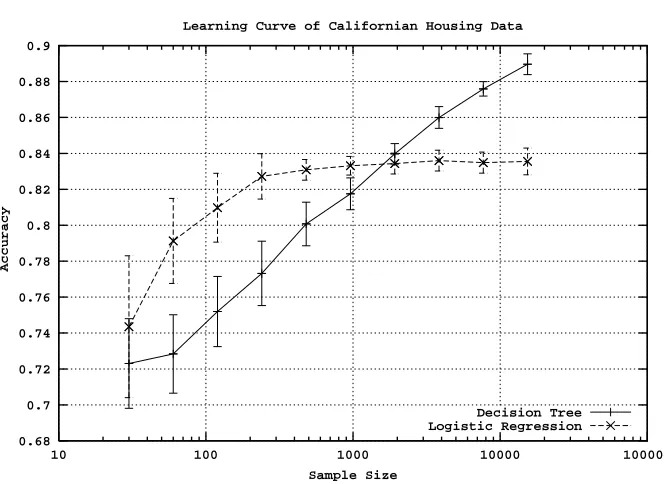
As mentioned above, the fundamental analytical tool that we use is the learning curve. Learning curves represent the generalization performance of the models produced by a learning algorithm, as a function of the size of the training set. Figure 1 shows two typical learning curves. For smaller training-set sizes the curves are steep, but the increase in accuracy lessens for larger training-set sizes. Often for very large training-set sizes this standard representation obscures small, but non-trivial, gains. Therefore to visualize the curves we use two transformations. First we use a log scale on the horizontal axis. Second, we start the graph at the accuracy of the smallest training-set size (rather than at zero). The transformation of the learning curves in Figure 1 is shown in Figure 2.
We produce learning curves for variants of tree induction and logistic regression based on 36 data sets. We now describe these data sets, the measures of accuracy we use (for the vertical axes of the learning curve plots), the technical details of how learning curves are produced, and the implementations of the learning algorithms and variants.
3.1 Data Sets
We selected 36 data sets representing binary classification tasks. In order to get learning curves of a reasonable length, each data set was required to have at least 700 observations. To this end, we chose many of the larger data sets from the UCI data repository (Blake and Merz, 2000) and
0 0.1 0.2 0.3 0.4 0.5 0.6 0.7 0.8 0.9
0 2000 4000 6000 8000 10000 12000 14000 16000
Accuracy
Sample Size
Learning Curve of Californian Housing Data
Decision Tree Logistic Regression
Figure 1: Typical learning curves
0.68 0.7 0.72 0.74 0.76 0.78 0.8 0.82 0.84 0.86 0.88 0.9
10 100 1000 10000 100000
Accuracy
Sample Size
Learning Curve of Californian Housing Data
Decision Tree Logistic Regression
from other learning repositories. We selected data drawn from real domains and avoided synthetic data. The rest were obtained from practitioners with real classification tasks with large data sets. Appendix B gives source details for all of the data sets.
We only considered tasks of binary classification, which facilitates the use of logistic regression and allows us to compute the area under the ROC curve, described below, which we rely on heavily in the analysis. Some of the two-class data sets are constructed from data sets originally having more classes. For example, the Letter-A data set and the Letter-V data set are constructed by taking the UCI letter data set, and using as the positive class instances of the letter “a” or instances of vowels, respectively. Finally, because of problems encountered with some of the learning programs, and the arbitrariness of workarounds, we avoided missing data for numerical variables. If missing values occurred in nominal values we coded them explicitly C4.5 has a special facility to deal with missing values, coded as “?”. In order to keep logistic regression and tree induction comparable, we chose a different code and modeled missing values explicitly as a nominal value. Only two data sets contained missing numerical data (Downsize and Firm Reputation). In those cases we excluded rows or imputed the missing value using the mean for the other variable values in the record. For a more detailed explanation see Appendix B.
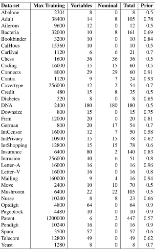
Table 1 shows the specification of the 36 data sets used in this study, including the maximum training size, the number of variables, the number of nominal variables, the total number of param-eters (1 for a continuous variable, number of nominal values minus one for each nominal variable), and the base rate (“prior”) of the more prevalent class (in the training set).
3.2 Evaluation Metrics
We compare performance using two evaluation metrics. First, we use classification accuracy (equiv-alently, undifferentiated error rate): the number of correct predictions on the test data divided by the number of test data instances. This has been the standard comparison metric used in studies of classifier induction in the machine learning literature.
Classification accuracy obviously is not an appropriate evaluation criterion for all classification tasks (Provost, Fawcett, and Kohavi, 1998). For this work we also want to evaluate and compare different methods with respect to their estimates of class probabilities. One alternative to classifi-cation accuracy is to use ROC (Receiver Operating Characteristic) analysis (Swets, 1988), which compares visually the classifiers’ performance across the entire range of probabilities. For a given binary classifier that produces a score indicating likelihood of class membership, its ROC curve de-picts all possible tradeoffs between true-positive rate (T P) and false-positive rate (FP). Specifically, any classification threshold on the score will classify correctly an expected percentage of truly pos-itive cases as being pospos-itive (T P) and will classify incorrectly an expected percentage of negative examples as being positive (FP). The ROC curve plots the observed T P versus F P for all possible classification thresholds. Provost and Fawcett (Provost and Fawcett, 1997, 2001) describe how pre-cise, objective comparisons can be made with ROC analysis. However, for the purpose of this study, we want to evaluate the class probability estimates generally rather than under specific conditions or under ranges of conditions. In particular, we concentrate on how well the probability estimates can rank cases by their likelihood of class membership. There are many applications where such ranking is more appropriate than binary classification.
proba-Table 1: Data sets
Data set Max Training Variables Nominal Total Prior
Abalone 2304 8 0 8 0.5
Adult 38400 14 8 105 0.78
Ailerons 9600 12 0 12 0.5
Bacteria 32000 10 8 161 0.69
Bookbinder 3200 10 0 10 0.84
CalHous 15360 10 0 10 0.5
CarEval 1120 6 6 21 0.7
Chess 1600 36 36 36 0.5
Coding 16000 15 15 60 0.5
Connects 8000 29 29 60 0.91
Contra 1120 9 7 24 0.93
Covertype 256000 12 2 54 0.7
Credit 480 15 8 35 0.5
Diabetes 320 8 0 8 0.65
DNA 2400 180 180 180 0.5
Downsize 800 15 0 15 0.75
Firm 12000 20 0 20 0.81
German 800 20 17 54 0.7
IntCensor 16000 12 7 50 0.58
IntPrivacy 10900 15 15 78 0.62
IntShopping 12800 15 15 78 0.6
Insurance 6400 80 2 140 0.83
Intrusion 256000 40 6 51 0.8
Letter–A 16000 16 0 16 0.96
Letter–V 16000 16 0 16 0.8
Mailing 160000 9 4 16 0.94
Move 2400 10 10 70 0.5
Mushroom 6400 22 22 105 0.5
Nurse 10240 8 8 23 0.66
Optdigit 4800 64 0 64 0.9
Pageblock 4480 10 0 10 0.9
Patent 1200000 6 2 447 0.57
Pendigit 10240 16 0 16 0.9
Spam 3500 57 0 57 0.6
Telecom 12800 49 0 49 0.62
bility distributions are not known. Instead, a set of instances is available, labeled with the true class, and comparisons are based on estimates of performance from these data. The Wilcoxon(-Mann-Whitney) nonparametric test statistic is appropriate for this comparison (Hand, 1997). The Wilcoxon measures, for a particular classifier, the probability that a randomly chosen class-0 case will be assigned a higher class-0 probability than a randomly chosen class-1 case. Therefore higher Wilcoxon score indicates that the probability ranking is generally better. Note that this evaluation side-steps the question of whether the probabilities are well calibrated.5
Another metric for comparing classifiers across a wide range of conditions is the area under the ROC curve (AUR) (Bradley, 1997); AUR measures the quality of an estimator’s classification performance, averaged across all possible probability thresholds. The AUR is equivalent to the Wilcoxon statistic (Hanley and McNeil, 1982), and is also essentially equivalent to the Gini coeffi-cient (Hand, 1997). Therefore, for this work we report the AUR when comparing class probability estimation.
It is important to note that AUR judges the relative quality of the entire probability-based rank-ing. It may be the case that for a particular threshold (e.g., the top 10 cases) a model with a lower AUR in fact is desirable.
3.3 Producing Learning Curves
In order to obtain a smooth learning curve with a maximum training size Nmaxand test size T we perform the following steps 10 times and average the resulting curves. The same training and test sets were used for all of the learning methods.
(1) Draw an initial sample Sallof size Nmax+T from the original data set. (We chose the test size
T to be between one-quarter and one-third of the original size of the data set.)
(2) Split the set Sallrandomly into a test set Stestof size T and keep the remaining Nmax observa-tions as a data pool Strain-sourcefor training samples.
(3) Set the initial training size N to approximately 5 times the number of parameters in the logistic model.
(4) Sample a training set Strainwith the current training size N from the data pool Strain-source. (5) Remove all data from the test set Stest that have nominal values that did not appear in the
training set. Logistic regression requires the test set to contain only those nominal values that have been seen previously in the training set. If the training sample did not contain the value “blue” for the variable color, for example, logistic regression cannot estimate a parameter for this dummy variable and will produce an error message and stop execution if a test example with color = “blue” appears. In comparison C4.5 splits the example probabilistically, and sends weighted (partial) examples to descendent nodes; for details see Quinlan (1993). We therefore remove all test examples that have new nominal values from Stest and create Stest,N
for this particular N. The amount of data rejected in this process depends on the distribution of nominal values, and the size of the test set and the current training set. However, we usually lose less than 10% of our test set.
(6) Train all models on the training set Strain and obtain their predictions for the current test set
Stest,N. Calculate the evaluation criteria for all models. (7) Repeat steps 3 to 6 for increasing training size N up to Nmax.
All samples in the outlined procedure are drawn without replacement. After repeating these steps 10 times we have for each method and for each training-set size 10 observations of each evaluation criterion. The final learning curves of the algorithms in the plots connect the means of the 10 evaluation-criterion values for each training-set size. We use the standard deviation of these values as a measure of the inherent variability of each evaluation criterion across different training sets of the same size, constructing error bars at each training-set size representing ±one standard deviation. In the evaluation we consider two models as different for a particular training-set size if the mean for neither falls within the error bars of the other.
We train all models on the same training data in order to reduce variation in the performance measures due to sampling of the training data. By the same argument we also use the same test set for all different training-set sizes (for each of the ten learning curves), as this decreases the variance and thereby increases the smoothness of the learning curve.
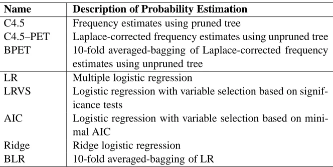
3.4 Implementation
In this section we describe the implementations of the learning methods. Appendix A describes tree induction and logistic regression in detail, including the variants studied below.
3.4.1 TREEINDUCTION
To build classification trees we used C4.5 (Quinlan, 1993) with the default parameter settings. To obtain probability estimates from these trees we used the frequency scores at the leaves. Our second algorithm, C4.5-PET (Probability Estimation Tree), uses C4.5 without pruning and estimates the probabilities as Laplace-corrected frequency scores (Provost and Domingos, 2003). The third algo-rithm in our comparison, BPET, performs a form of bagging (Breiman, 1996) using C4.5. Specifi-cally, averaged-bagging estimates 10 unpruned trees from 10 bootstrap subsamples of the training data and predicts the mean of the probabilities.6 Details of the implementations are summarized in Table 2.
3.4.2 LOGISTIC REGRESSION
Logistic regression was performed using the SAS program PROC LOGISTIC. A few of the data sets exhibited quasicomplete separation, in which there exists a linear combination of the predictors
β0x such thatβ0x
i≥0 for all i where yi=0 andβ0xi≤0 for all i where yi=1, with equality holding for at least one observation with yi=0 and at least one observation with yi=1.7 In this situation a 6. This is in contrast to standard bagging, for which votes are tallied from the ensemble of models and the class with the majority/plurality is predicted. Averaged-bagging allows us both to perform probability estimation and to perform classification (thresholding the estimates at 0.5).
Table 2: Implementation Details
Name Description of Probability Estimation C4.5 Frequency estimates using pruned tree
C4.5–PET Laplace-corrected frequency estimates using unpruned tree BPET 10-fold averaged-bagging of Laplace-corrected frequency
estimates using unpruned tree LR Multiple logistic regression
LRVS Logistic regression with variable selection based on signif-icance tests
AIC Logistic regression with variable selection based on mini-mal AIC
Ridge Ridge logistic regression BLR 10-fold averaged-bagging of LR
unique maximum likelihood estimate does not exist, since the log-likelihood increases to a constant as at least one parameter becomes infinite. Quasicomplete separation is more common for smaller data sets, but it also can occur when there are many qualitative predictors that have many nominal values, as is sometimes the case here. SAS stops the likelihood iterations prematurely with an error flag when it identifies quasicomplete separation (So, 1995), which leads to inferior performance. For this reason, for these data sets the logistic regression models are fit using the glm() function of the statistical package R (Ihaka and Gentleman, 1996), since that package continues the maximum likelihood iterations until the change in log-likelihood is below a preset tolerance level.
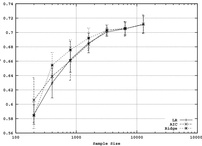
Logistic regression with variable selection based on significance tests was also performed using PROC LOGISTIC. In addition, a variable selection variant using AIC (Akaike, 1974) and a ridge logistic regression variant (le Cessie and van Houwelingen, 1992) were implemented in the statis-tical package R.8Due to computational constraints such as memory limits, the R-based variants do not execute for very large data sets and so we cannot report results for those cases. Details of the implementation are summarized in Table 2. We discuss the variable-selection procedures in more detail below, when we present the results.
For bagged logistic regression, similarly to bagged tree induction, we used 10 subsamples, taken with replacement, of the same size as the original training set. We estimated 10 logistic regression models and took the mean of the probability predictions on the test set of those 10 models as the final probability prediction for the test set. The issue of novel nominal values in the test set again creates problems for bagged logistic regression. As was noted earlier, logistic regression requires all levels of nominal variables that appear in the test set to have also appeared in the training set. In order to guarantee this for each of the 10 sub-training sets, a base set was added to the 10 sub-training sets. This base set contains at least two observations containing each nominal value appearing in the test set.
4. Variants of Methods: Learning Curve Analysis
In this section we investigate the usefulness of the different variants of the learning algorithms. We first focus on tree induction and then consider logistic regression.
4.1 Variants of Tree Induction
We compare the learning curves to examine the effects of pruning, the Laplace correction, and bag-ging. C4.5 (and tree-induction generally) prunes learned trees in order to compensate for overfitting by the tree-growing process. Error-based pruning (as in C4.5) can hurt probability estimation based on trees, because it eliminates distinctions in estimates that would not affect classification (Provost and Domingos, 2003). For example, two sibling leaves with probability estimates of 0.8 and 0.9 both would yield a positive classification; however, the different scores may significantly improve the quality of rankings of cases by class-membership probability. The Laplace correction is an at-tempt to deal with errors in scores due to the smaller samples at the leaves of unpruned trees, and due to the overly extreme bias in the probabilities, as discussed in Appendix A. Bagging reduces variance, which is important because variance leads to estimation errors as well as classification errors (Friedman, 1997).
The ability of the Laplace correction and bagging to improve probability estimation of induced trees has been noted previously. Bauer and Kohavi (1999) show improvements using mean-squared error from the true (0/1) class; Provost, Fawcett, and Kohavi (1998) present ROC curves that show similar results, and Provost and Domingos (2003) show similar results using AUR. Our results are consistent with expectations.
PRUNING (C4.5VERSUSC4.5-PET)
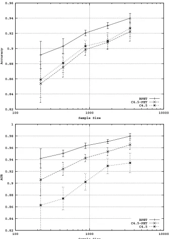
For classification accuracy, pruning9 improves the performance in ten cases (the win-tie-loss tally, based on whether the mean of the error measure for one method was within the error bound of the other, was 10-25-1). However, the improvements are small in most cases. The top plot of Figure 3 shows a typical case of accuracy learning curves (Spam data set).
The performance comparison of C4.5 and C4.5-PET is systematically reversed for producing ranking scores (AUR). The Laplace transformation/not-pruning combination improves the AUR in twenty-two cases and is detrimental in only two cases (IntPriv and IntCensor) (win-tie-loss: 22-12-2). The lower plot of figure 3 shows this reversal on the same data set (Spam). Notice that, in contrast to accuracy, the difference in AUR is considerable between C4.5 and C4.5-PET.
BAGGING(BPETVERSUSC4.5)
Averaged-bagging often improves accuracy, sometimes substantially. The win-tie-loss tally is 10-21-5 in favor of bagging over C4.5. In terms of producing ranking scores (AUR), BPET was never worse than C4.5, with a 24-12-0 result.
0.82 0.84 0.86 0.88 0.9 0.92 0.94 0.96
100 1000 10000
Accuracy
Sample Size
BPET C4.5-PET C4.5
0.82 0.84 0.86 0.88 0.9 0.92 0.94 0.96 0.98 1
100 1000 10000
AUR
Sample Size
BPET C4.5-PET C4.5
BAGGING(BPETVERSUSC4.5-PET)
The only difference between BPET and C4.5-PET is the averaged-bagging. Both use Laplace cor-rection on unpruned trees. BPET dominates this comparison for both accuracy and probability estimation (16-18-2 for accuracy and 15-19-2 for AUR). The two data sets where bagging hurts are Mailing and Abalone. However, looking ahead, in both these cases tree induction did not perform well compared to logistic regression.
Based on these results, for the comparison with logistic regression in Section 5, we use two methods: C4.5-PET (Laplace corrected and not pruned) and BPET. Keep in mind that this may underrepresent C4.5’s performance slightly when it comes to classification accuracy, since with pruning regular C4.5 typically is slightly better. However, the number of runs in Section 5 is huge. Both for comparison and for computational practicability it is important to limit the number of learning algorithms. Moreover, we report surprisingly strong results for C4.5 below, so our choice here is conservative.
4.2 Variants of Logistic Regression
In this section we discuss the properties of the three variants of logistic regression that we are con-sidering (no variable selection, variable selection, and ridge regression). Our initial investigations into variable selection were done using SAS PROC LOGISTIC, since it could be applied to very large data sets. We investigated both forward and backward selection, although backward selec-tion is often less successful than forward selecselec-tion because the full model fit in the first step is the model most likely to result in a complete or quasicomplete separation of response values. We did not use the STEPWISE setting in SAS, which combines both forward and backward stepping, or the SCORE setting, which looks at all possible regression models, because they are impracticable computationally.
SAS also supports a variation of backward and forward stepping based on the Pearson goodness– of–fit statistic X2(see Appendix A, equation (4)). In the case of forward stepping the algorithm stops adding variables when X2becomes insignificant (that is, the null hypothesis that the logistic regres-sion model fits the data is not rejected), while for backward stepping variables are removed until
X2becomes significant (that is, the null hypothesis that the logistic regression model fits the data is rejected). Backward selection also can be done using the computational algorithm of Lawless and Singhal (1978) to compute a first-order approximation to the remaining slope estimates for each subsequent elimination of a variable from the model. Variables are removed from the model based on these approximate estimates. The FAST option is extremely efficient because the model is not refitted for every variable removed.
0.65 0.7 0.75 0.8 0.85 0.9 0.95
100 1000 10000
Accuracy
Sample Size
LR AIC Ridge
Figure 4: Accuracy learning curves of logistic regression variants for the Firm Reputation data set, illustrating the stronger performance of model-selection-based logistic regression for smaller sample sizes.
Model selection using AIC does better, more often resulting in improved performance relative to using the full logistic regression model, particularly for smaller sample sizes. Evidence of this is seen, for example, in the Adult, Bacteria, Mailing, Firm Reputation, German, Spam, and Tele-com data sets. Figure 4, which shows the logistic regression accuracy learning curves for the Firm Reputation data set, gives a particularly clear example, where the AIC learning curve is consistently higher than that for ordinary logistic regression, and distinctly higher up to sample sizes of at least 1000. Corresponding plots for AUR are similar. Model selection also can lead to poorer perfor-mance, as it does in the CalHous, Coding, and Optdigit data sets. However, as was noted earlier, AIC-based model selection is infeasible for large data sets.10
The case for ridge logistic regression is similar, but the technique was less successful. While ridge logistic regression was occasionally effective for small samples (see, for example, Figure 5, which refers to the Intshop data set), for the majority of data sets using it resulted in similar or poorer performance compared to the full regression. We will therefore not discuss it further. Note, however, that we used one particular method of choosing the ridge parameterλ; perhaps some other choice would have worked better, so our results should not be considered a blanket dismissal of the idea of ridge logistic regression.
Bagging is systematically detrimental to performance for logistic regression. In contrast to the observation regarding bagging for trees, for logistic regression bagging seems to shift the learning
0.56 0.58 0.6 0.62 0.64 0.66 0.68 0.7 0.72 0.74
100 1000 10000 100000
Accuracy
Sample Size
LR AIC Ridge
Figure 5: Accuracy learning curves of logistic regression variants for the Internet shopping data set, illustrating a situation where ridge logistic regression is effective for small sample sizes.
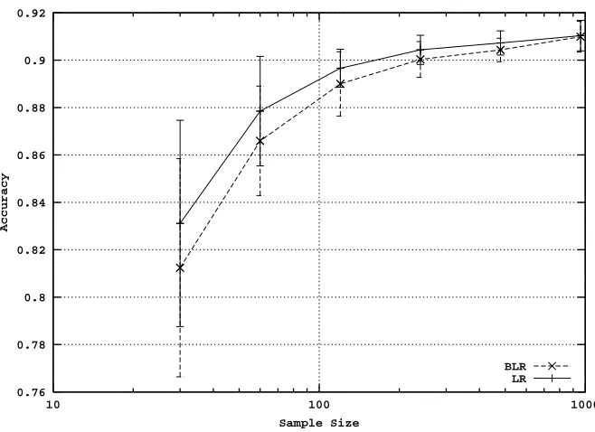
curve to the right. Note that bagging trains individual models with substantially fewer examples (approximately 0.63n distinct original observations, where n is the training-set size). Therefore when the learning curve is steep, the individual models will have considerably lower accuracies than the model learned from the whole training set. In trees, this effect is more than compensated for by the variance reduction, usually yielding a net improvement. However, logistic regression has little variance, so all bagging does is to average the predictions of a set of poor models (note that bagging does seem to result in a small improvement over the accuracy produced with 63% of the data). B ¨uhlman and Yu (2002) discuss the properties of bagging theoretically, and show that it should help for “hard threshold” methods, but not for “soft threshold” methods. Logistic regression falls into their “soft threshold” category.
In sum, our conclusion for logistic regression is quite different from that for tree induction (in the previous section). For larger training-set sizes, which are at issue in this paper, none of the variants improve considerably on the basic algorithm. Indeed, bagging is detrimental. Therefore, for the following study we only consider the basic algorithm. It should be noted, however, that this decision apparently has no effect on our conclusions concerning the relative effectiveness of logistic regression and tree induction, since even for the smaller data sets a “which is better” assessment of the basic logistic regression algorithm compared to tree induction is the same as that of the best variant of logistic regression.
0.76 0.78 0.8 0.82 0.84 0.86 0.88 0.9 0.92
10 100 1000
Accuracy
Sample Size
BLR LR
Figure 6: Accuracy learning curves for the Californian housing data set, illustrating the negative impact of bagging on logistic regression performance.
number of parameters does not grow with the sample size, such as with logistic regression). As the data set gets larger, eventually the parameters of the model are estimated as accurately as they can be, with standard error (virtually) zero. At this point additional data will not change anything, and the learning curve must level off.
5. Differences Between Tree Induction and Logistic Regression: Learning Curve Analysis
We now present our main experimental analysis. We compare the learning curve performance of the three chosen methods, C4.5-PET (Laplace-corrected, unpruned probability estimation tree), BPET (bagged C4.5-PET), and multiple logistic regression, as tools for building classification models and models for class probability estimation. Here and below, we are interested in comparing the perfor-mance of tree induction with logistic regression, so we generally will not differentiate in summary statements between BPET and PET, but just say “C4.” In the graphs we show the performance of all of the methods.
“X crosses” indicates that a method of type X is not better for smaller training-set sizes, but is better for larger training-set sizes. “Indistinguishable” means that at the end of the learning curve with the maximal training set we cannot identify one method (logistic regression or a tree induction) as the winner.
One data set (Adult) is classified as “Mixed.” In this case we found different results for Accuracy (C4 crosses) and AUR (LR dominates). We discuss the reason and implications of this result more generally in Section 5.3.
As described above, the area under the ROC curve (AUR) is a measure of how well a method can separate the instances of the different classes. In particular, if you rank the test instances by the scores given by the model, the better the ranking the larger the AUR. A randomly shuffled ranking will give an AUR of (near) 0.5. A perfect ranking (perfectly separating the classes into two groups) gives an AUR of 1.0. Therefore, the maximum AUR achieved by any method (max-AUR) can be considered an estimation of the fundamental separability of the signal from the noise—estimated with respect to the modeling methods available. If no method does better than random (max-AUR = 0.5), then as far as we can tell it is not possible to separate the signal (and it does not make sense to compare learning algorithms). If some method performs perfectly (max-AUR = 1.0), then the signal and noise can be separated perfectly.
Max-AUR is similar to an estimation of the Bayes rate (the minimum possible misclassifica-tion error rate), with a crucial difference: max-AUR is independent of the base rate—the marginal (“prior”) probability of class membership—and the Bayes rate is not. This difference is crucial, be-cause max-AUR can be used to compare different data sets with respect to the separability of signal from noise. For example, a data set with 99.99% positive examples should engender classification accuracy of at least 99.99%, but still might have max-AUR = 0.5 (the signal cannot be separated from the noise). The data sets in Table 3 are presented in order of decreasing max-AUR—the most separable at the top, and the least separable at the bottom.
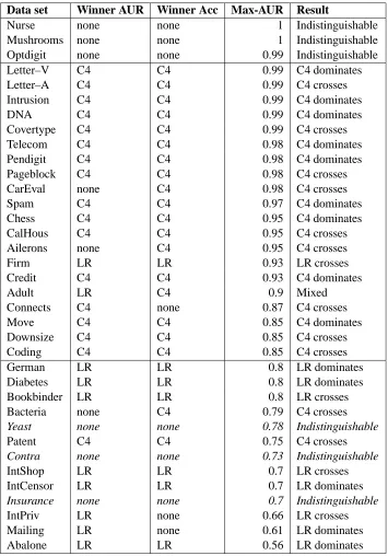
We have divided the results in Table 3 into three groups, indicated by horizontal lines. The relative performance of the classifiers appears to be fundamentally different in each group.
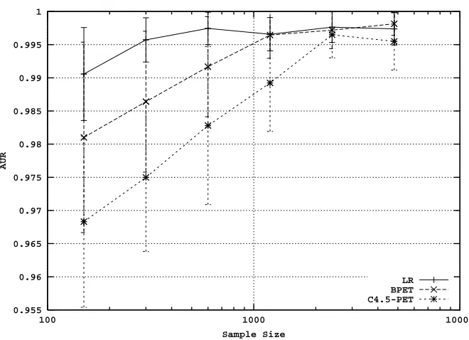
The topmost group, comprising Mushroom, Nurse, and Optdigit, contains three situations where the signal-from-noise separability is extremely high. All methods quickly attain accuracy and AUR values over .99, and are indistinguishable. The learning curves for AUR for Optdigit are shown in Figure 7. For purposes of comparison, these data sets are “too easy,” in the sense that all methods isolate the structure completely, very quickly. Since these data sets do not provide helpful informa-tion about differences in effectiveness between methods, we will not consider them further.
Remarkably, the comparison of the methods for the rest of the data sets can be characterized quite well by two aspects of the data: the separability of the signal from the noise, and the size of the data set. As just described, we measure the signal separability using max-AUR. We consider two cases: max-AUR≤0.8 (lower signal separability) and max-AUR≥0.85 (higher signal sepa-rability). The max-AUR split is reflected in the lower, horizontal division in the table. No data sets have 0.8<max-AUR<0.85.
5.1 Data with High Signal-from-Noise Separability
Table 3: Results of learning curve analyses.
Data set Winner AUR Winner Acc Max-AUR Result
Nurse none none 1 Indistinguishable
Mushrooms none none 1 Indistinguishable
Optdigit none none 0.99 Indistinguishable
Letter–V C4 C4 0.99 C4 dominates
Letter–A C4 C4 0.99 C4 crosses
Intrusion C4 C4 0.99 C4 dominates
DNA C4 C4 0.99 C4 dominates
Covertype C4 C4 0.99 C4 crosses
Telecom C4 C4 0.98 C4 dominates
Pendigit C4 C4 0.98 C4 dominates
Pageblock C4 C4 0.98 C4 crosses
CarEval none C4 0.98 C4 crosses
Spam C4 C4 0.97 C4 dominates
Chess C4 C4 0.95 C4 dominates
CalHous C4 C4 0.95 C4 crosses
Ailerons none C4 0.95 C4 crosses
Firm LR LR 0.93 LR crosses
Credit C4 C4 0.93 C4 dominates
Adult LR C4 0.9 Mixed
Connects C4 none 0.87 C4 crosses
Move C4 C4 0.85 C4 dominates
Downsize C4 C4 0.85 C4 crosses
Coding C4 C4 0.85 C4 crosses
German LR LR 0.8 LR dominates
Diabetes LR LR 0.8 LR dominates
Bookbinder LR LR 0.8 LR crosses
Bacteria none C4 0.79 C4 crosses
Yeast none none 0.78 Indistinguishable
Patent C4 C4 0.75 C4 crosses
Contra none none 0.73 Indistinguishable
IntShop LR LR 0.7 LR crosses
IntCensor LR LR 0.7 LR dominates
Insurance none none 0.7 Indistinguishable
IntPriv LR none 0.66 LR crosses
Mailing LR none 0.61 LR dominates
0.955 0.96 0.965 0.97 0.975 0.98 0.985 0.99 0.995 1
100 1000 10000
AUR
Sample Size
LR BPET C4.5-PET
Figure 7: AUR learning curves for the Optdigit data set, illustrating a situation where all methods achieve high performance quickly.
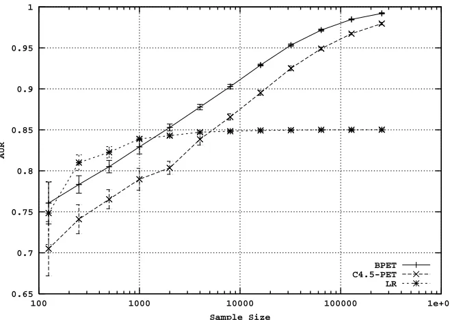
training sets (C4’s win-tie-loss record is 19-1-1). In some cases the tree learning curve dominates; Letter-V is a good example of this situation, as shown in Figure 8.
Here the logistic regression learning curve initially is slightly steeper than that of the tree, but the logistic regression curve quickly levels off, while the tree keeps learning, achieving far higher accuracy than the logistic regression. Move, Pendigit, and Spam are roughly similar.
In the other situations, logistic regression’s advantage for smaller data sets extends further, so that it is clearly better for smaller data sets, but eventually tree induction surpasses logistic regres-sion both in terms of accuracy and AUR. Ailerons, Coding, Covertype, and Letter-A provide good examples of this situation. The AUR curves for Covertype are shown in Figure 9.
When will one see a domination of one method, and when will there be a crossing? We do not have a definitive answer, but it is reasonable to expect a combination of two factors. First, how “linear” is the true concept to be learned? If there are fewer non-linearities and there is little noise, then logistic regression will do better early on (relative to the number of parameters, of course); tree induction will need more data to reach the necessary complexity. Second, it simply depends on where you start looking: what is the smallest training-set size in relation to the number of parameters? If you start with larger training sets, trees are more likely to dominate.
0.65 0.7 0.75 0.8 0.85 0.9 0.95 1
10 100 1000 10000 100000
Accuracy
Sample Size
LR BPET C4.5-PET
Figure 8: Accuracy learning curves for the Letter-V data set, illustrating a situation where C4 dom-inates.
0.65 0.7 0.75 0.8 0.85 0.9 0.95 1
100 1000 10000 100000 1e+06
AUR
Sample Size
BPET C4.5-PET LR
curves cross the logistic regression curves, the crossover point for accuracy comes at the same point or earlier than the crossover point for AUR, but not later. An alternative view is that logistic regres-sion apparently is better tuned for probability ranking than it is for classification. Given that the method is specifically designed to model probabilities (with classification as a possible side-effect of that probability estimation), this also is not surprising.
Evidence of this can be seen in Adult, Ailerons, and Letter-A, where the crossover points of the AUR learning curves have not been reached (although for each, the trajectories of the curves suggest that with more data the tree would eventually become the winner). The cases for Adult for both accuracy and AUR are shown in Figure 10.
5.2 Data with Low Signal-from-Noise Separability
The lower signal-separability situation (max-AUR≤0.8) is slightly more complicated. Sometimes it is impossible to distinguish between the performances of the methods. Examples of this (italicized in Table 3) include Contraception, Insurance and Yeast. For these data sets it is difficult to draw any conclusions, in terms of either accuracy or AUR, since the curves tend to be within each other’s error bars. Figure 11 illustrates this for the Contra data set.
When the methods are distinguishable logistic regression is clearly the more effective method, in terms of both accuracy and AUR. Ten data sets fall into this category. Logistic regression’s win-tie-loss record here is 8-1-1 for AUR and 6-2-2 for accuracy. Examples of this are Abalone, Bookbinder, Diabetes, and the three Internet data sets (IntCensor, IntPrivacy, and IntShopping). Figure 12 shows this case for the IntCensor data set.
As was true in the higher signal-separability situation, logistic regression fares better (compar-atively) with respect to AUR than with respect to accuracy. This is reflected in a more clear gap between logistic regression and the best tree method in terms of AUR compared to accuracy; for example, for IntPriv and Mailing logistic regression is better for AUR, but not for accuracy.
5.3 The Impact of Data-Set Size
The Patent data set is an intriguing case, which might be viewed as an exception. In particular, although it falls into the low signal-separability category, C4 is the winner for accuracy and for AUR. This data set is by far the largest in the study, and at an extremely large training data size the induced tree becomes competitive and beats the logistic model. As shown in Figure 13, the curves cross when the training sets contain more than 100,000 examples.
The impact of data-set size on these results is twofold. First, in this study we use max-AUR as a proxy for the true (optimal) separability of signal from noise. However, even with our large data sets, in almost no case did the AUR learning curve level off for tree induction. This suggests that we tend to underestimate the separability.
0.77 0.78 0.79 0.8 0.81 0.82 0.83 0.84 0.85 0.86 0.87
100 1000 10000 100000
Accuracy
Sample Size
LR BPET C4.5-PET
0.8 0.82 0.84 0.86 0.88 0.9 0.92
100 1000 10000 100000
AUR
Sample Size
LR BPET C4.5-PET
0.55 0.6 0.65 0.7 0.75 0.8
10 100 1000 10000
AUR
Sample Size
LR BPET C4.5-PET
Figure 11: AUR learning curves for the Contra data set, illustrating low signal separability and indistinguishable performance.
0.52 0.54 0.56 0.58 0.6 0.62 0.64 0.66 0.68 0.7 0.72 0.74
100 1000 10000 100000
AUR
Sample Size
LR BPET C4.5-PET
0.5 0.55 0.6 0.65 0.7 0.75 0.8
100 1000 10000 100000 1e+06 1e+07
AUR
Sample Size
BPET C4.5-PET LR
Figure 13: AUR learning curves for the the Patent data set, illustrating a situation where tree induc-tion surpasses logistic regression for extremely large training-set sizes.
6. Discussion and Implications
Let us consider these results in the context of prior work. A comprehensive experimental study of the performance of induction algorithms is described by Lim, Loh, and Shih (2000). They show that averaged over 32 data sets, logistic regression outperforms C4.5. Specifically, the classification error rate for logistic regression is 7% lower than that of C4.5. Additionally, logistic regression was the second best algorithm in terms of consistently low error rates: it is not significantly different from the minimum error rate (of the 33 algorithms they compare) on 13 of the 32 data sets. The only algorithm that fared better (15/32) was a complicated spline-based logistic regression that was extremely expensive computationally. In comparison, C4.5 was the 17th best algorithm in these terms, not differing from the minimum error rate on only 7 of the data sets.
Our results clarify and augment the results of that study. First of all, we use bagging, which improves the performance of C4.5 consistently. More importantly, Lim et al. concentrate on UCI data sets without considering data-set size. Their training-set sizes are relatively small; specifically, their average training-set size is 900 (compare with an average of 60000 at the right end of the learning curves of the present study; median=12800).11 Although C4 would clearly “win” a straight comparison over all of the data sets in our study, examining the learning curves shows that C4 often needs more data than logistic regression to achieve its ultimate classification accuracy.
This leads to a more general observation, which bears on many prior studies by machine learning researchers comparing induction algorithms on fixed-size training sets. In only 14 of 36 cases
0.4 0.45 0.5 0.55 0.6 0.65 0.7 0.75 0.8 0.85
100 1000 10000 100000
AUR
Sample Size
LR BPET C4.5-PET
Figure 14: AUR learning curves for the Bacteria data set. The AUR of Bacteria has already reached 0.79 and tree induction has not leveled off. One could speculate that BPET will achieve AUR>0.8.
does one method dominate for the entire learning curve. Thus, it is not appropriate to conclude from a study with a single training-set size that one algorithm is “better” (in terms of predictive performance) than another for a particular domain. Rather, such conclusions must be tempered by examining whether the learning curves have reached plateaus. If not, one only can conclude that for the particular training-set size used, one algorithm performs better than another. This also has implications for practices such as using hold-out sets for comparison, as discussed below.
In this study of two standard learning methods we can see a clear criterion for when each algo-rithm is preferable: C4 for high-separability data and logistic regression for low-separability data. Curiously, the two clear exceptions in the low signal-separability case (the cases where C4 beats logistic regression), Patent and Bacteria, may not be exceptions at all; it may simply be that we still do not have enough data and we underestimate the true max-AUR. For both of these cases, the C4 learning curves do not seem to be leveling off even at the largest training-set sizes. Figure 13 shows this for the Patent data set and Figure 14 shows this for the Bacteria data set. In both cases, given more training data, the maximum AUR seems likely to exceed 0.8; therefore, these data may actu-ally fall into the high signal-separability category. If that were so, the C4-tie-LR record for accuracy for the high-separability data sets would be 21-1-1, and for the (large-enough) low-separability data sets 0-2-6.
They do not show learning curves, so we cannot conclude whether tree induction would perform better with more data. However, they state clearly (pp. 2507-8), “We suspect that adaptive non-linear methods are most useful in problems with high signal-to-noise ratio, sometimes ocurring in engineering and physical science. In human studies, the signal-to-noise ratio is often quite low (as it is here), and hence the modern methods may have less to offer.”
We are not aware of this seemingly straightforward relationship being shown in previous ex-perimental comparisons, even though studies have compared logistic regression to tree induction. Many comparative studies simply have not looked for such relationships. However, some have. Notably, the Statlog project (King, Feng, and Sutherland, 1995) looked specifically at the charac-teristics of the data that indicate the preferability of different types of induction algorithms. They include tree induction and logistic regression in their comparison, and relate the differences in their performances to the skew and kurtosis of the predictor variables, which relate to the (multivari-ate) normality of the data. Thus, not surprisingly, tree induction should be preferable when the distributional assumptions of the logistic regression are not satisfied. In theory, logistic regression should be preferable when they are—and indeed, for simulated data generated by multivariate class-conditional Normal models with equal covariance matrices, for which logistic regression is the right model, the performance of logistic regression approaches the Bayes rate and the true max-AUR, as expected. Tree induction never outperforms logistic regression.
However, given enough data, tree-based models can approximate non-axis-parallel class-probability boundaries arbitrarily closely (see the demonstration by Provost and Domingos, 2003). So, even when logistic regression is the right model, with enough data tree induction may be able to perform comparably, and generalization performance will be indistinguishable. If in addition, the correct logistic-regression model can separate the classes cleanly, then the indistinguishable generalization performance will be very good (as for the top three data sets in Table 3).
For data sets for which the logistic regression model is inadequate, when separability is high, the highly nonlinear nature of tree induction allows it to identify and exploit additional structure. On the other hand, when separability is low, the massive search performed by tree induction leads it to identify noise as signal, resulting in a deterioration of performance. It is a statistical truism that “All models are wrong, but some are useful” (Box, 1979, p. 202); this is particularly true when the signal is too difficult to distinguish from the noise to allow identification of the “correct” relationship. The general curve-crossing patterns we see concur with prior simulation studies showing learned linear models out-performing more complex learned models for small data sets, even when the more complex models better represent the true concept to be learned (Flury and Schmid, 1994; Domingos and Pazzani, 1997).
A limitation of our study is that we used the default parameters of C4.5. For example, the “-m” parameter specifies when to stop splitting, based on the size of leaves. Quinlan (1993) notes that the default value may not be best for noisy data. Therefore, one might speculate that with a better parameter setting, C4.5 might be more competitive with logistic regression for the low-separability data. Although the focus of this paper was the “off-the-shelf” algorithms, we have experimented systematically with the “-m” parameter on a large, high-noise data set (Mailing). The results do not draw our current conclusions into question.
0.72 0.74 0.76 0.78 0.8 0.82 0.84 0.86 0.88 0.9
10 100 1000 10000 100000
Accuracy
Sample Size
LR BPET Hybrid: LR -> BPET
Figure 15: Accuracy learning curves for a hybrid model on the California Housing data set.
up the analysis. These results show clearly that this practice can be misleading for many domains, if the relative shapes of the learning curves are not taken into account as well.
We also believe that the signal-separability categorization can be useful in cases where one wants to reduce the computational burden of comparing learning algorithms on large data.12 In particular, consider the following strategy.
1. Run C4.5-PET with the maximally feasible training-set size. For example, use all of the data available or all that will run well in main memory. C4.5 typically is a very fast induction alternative (cf., Lim, Loh, and Shih, 2000).
2. If the resultant AUR is high (0.85 or greater) continue to explore tree-based (or other non-parametric) options (for example, BPET, or methods that can deal with more data than can fit in main memory (Provost and Kolluri, 1999)).
3. If the resultant AUR is low, try logistic regression.
An alternative strategy is to build a hybrid model. Figure 15 shows the performance of tree induction on the California Housing data set, where tree building takes the probability estimation from a logistic regression model as an additional input variable. Note that the hybrid model tracks with each model in its region of dominance. In fact, around the crossing point, the hybrid model is substantially better than either alternative. While we are not aware of this particular hybrid model being proposed, nor this type of learning-curve performance being observed, there has been prior work on combining tree induction and logistic regression, for example using logistic models at the nodes of the tree and using leaf identifiers as dummies in the logistic regression (Steinberg and Cardell, 1998). A full review is beyond the scope of this article.
Another limitation of this study is that by focusing on the AUR, we are only examining proba-bility ranking, not probaproba-bility estimation. Logistic regression could perform better in the latter task, since that is what the method is designed for.
7. Conclusion
By using real data sets of very different sizes, with different levels of noise, we have been able to identify several broad patterns in the relative performance of tree induction and logistic regression. In particular, we see that the highly nonlinear nature of trees allows tree induction to exploit structure when the signal separability is high. On the other hand, the smoothness (and resultant low variance) of logistic regression allows it to perform well when signal separability is low.
Within the logistic regression family, we see that once the training sets are reasonably large, standard multiple logistic regression is remarkably robust, in the sense that different variants we tried do not improve performance (and bagging hurts performance). In contrast, within the tree induction family the different variants continue to make a difference across the entire range of training-set sizes: bagging usually improves performance, pruning helps for classification, and not pruning plus Laplace smoothing helps for scoring.13 Other approaches to reducing the variability of tree methods have also been suggested, and it is possible that these improvements would carry over to the problems and data sets examined here; see, for example, the work of Bloch, Olshen, and Walker (2002), Chipman, George, and McCulloch (1998), Hastie and Pregibon (1990), and LeBlanc and Tibshirani (1998).
We also have shown that examining learning curves is essential for comparisons of induction algorithms in machine learning. Without examining learning curves, claims of superior performance on particular “domains” are questionable at best. To emphasize this point, we calculated the C4-tie-LR records that would be achieved on this (same) set of domains, if data-set sizes had been chosen particularly well for each method. For accuracy, we can achieve a C4-tie-LR record of 22-13-1 by choosing data-set sizes favorable to C4. By choosing data-set sizes favorable to LR, we can achieve a record of 8-14-14. Similarly, for AUR, choosing well for C4 we can achieve a record of 23-11-2. Choosing well for LR we can achieve a record of 10-9-17. Therefore, it clearly is not appropriate, from simple studies with one data-set size (as with most experimental comparisons), to draw conclusions that one algorithm is better than the other for the corresponding domains or tasks. These results concur with recent results (Ng and Jordan, 2001) comparing discriminative and generative versions of the same model (viz., logistic regression and naive Bayes), which show that learning curves often cross.
These results also call into question the practice of experimenting with smaller data sets (for ef-ficiency reasons) to choose the best learning algorithm, and then “scaling up” the learning with the chosen algorithm. The apparent superiority of one method over another for one particular sample size does not necessarily carry over to larger samples (from the same domain). Similarly, con-clusions from experimental studies conducted with certain training-set/test-set partitions (such as two-thirds/one-third) many not even generalize to the source data set! Consider Patent, as shown in Figure 13.
A corollary observation is that even for very large data-set sizes, the slope of the learning curves remains distinguishable from zero. Catlett (1991) concluded that learning curves continue to grow,
on several large-at-the-time data sets (the largest with fewer than 100,000 training examples).14 Provost and Kolluri (1999) suggest that this conclusion should be revisited as the size of data sets that can be processed (feasibly) by learning algorithms increases. Our results provide a contem-porary reiteration of Catlett’s. On the other hand, our results seemingly contradict conclusions or assumptions made in some prior work. For example, Oates and Jensen (1997) conclude that classification-tree learning curves level off, and Provost, Jensen, and Oates (1999) replicate this finding and use it as an assumption of their sampling strategy. Technically, the criterion for a curve to have reached a plateau in these studies is that there be less than a certain threshold (one per-cent) increase in accuracy from the accuracy with the largest data-set size; however, the conclusion often is taken to mean that increases in accuracy cease. Our results show clearly that this latter interpretation is not appropriate even for our largest data-set sizes.
Finally, before undertaking this study, we had expected to see crossings in curves—in particular, to see the tree induction’s relative performance improve for larger training-set sizes. We did not expect such a clean-cut characterization of the performance of the learners in terms of the data sets’ signal separability. Neither did we expect such clear evidence that the notion of how large a data set is must take into account the separability of the data. Looking forward, we believe that reviving the learning curve as an analytical tool in machine learning research can lead to other important, perhaps surprising insights.
Acknowledgments
We thank Batia Wiesenfeld, Rachelle Sampson, Naomi Gardberg, and all the contributors to (and librarians of) the UCI repository for providing data. We also thank Tom Fawcett for writing and sharing the BPET software, Ross Quinlan for all his work on C4.5, Pedro Domingos for helpful dis-cussions about inducing probability estimation models, and IBM for a Faculty Partnership Award. PROC LOGISTIC software is copyright, SAS Institute Inc. SAS and all other SAS Institute Inc. product or service names are registered trademarks or trademarks of SAS Institute Inc., Cary, NC, USA.
This work is sponsored in part by the Defense Advanced Research Projects Agency (DARPA) and Air Force Research Laboratory, Air Force Materiel Command, USAF, under agreement number F30602-01-2-585. The U.S. Government is authorized to reproduce and distribute reprints for Gov-ernmental purposes notwithstanding any copyright annotation thereon. The views and conclusions contained herein are those of the authors and should not be interpreted as necessarily represent-ing the official policies or endorsements, either expressed or implied, of the Defense Advanced Research Projects Agency (DARPA), the Air Force Research Laboratory, or the U.S. Government.
Appendix A. Appendix: Algorithms for the Analysis of Binary Data
We describe here tree induction and logistic regression in more detail, including several variants examined in this paper. The particular implementations used are described in detail in Section 3.4.
A.1 Tree Induction for Classification and Probability Estimation
The terms “decision tree” and “classification tree” are used interchangeably in the literature. We use “classification tree” here, in order that we can distinguish between trees intended to produce clas-sifications, and those intended to produce estimations of class probability (“probability estimation trees”). When we are talking about the building of these trees, which for our purposes is essentially the same for classification and probability estimation, we simply say “tree induction.”
A.1.1 BASICTREE INDUCTION
Classification-tree learning algorithms are greedy, “recursive partitioning” procedures. They begin by searching for the single predictor variable xτ1 that best partitions the training data (as determined
by some measure). This first selected predictor, xτ1, is the root of the learned classification tree.
Once xτ1is selected, the training data are partitioned into subsets satisfying the values of the variable. Therefore, if xτ1 is a binary variable, the training data set is partitioned into two subsets.
The classification-tree learning algorithm proceeds recursively, applying the same procedure to each subset of the partition. The result is a tree of predictor variables, each splitting the data further. Different algorithms use different criteria to evaluate the quality of the splits produced by various predictors. Usually, the splits are evaluated by some measure of the “purity” of the resultant subsets, in terms of the outcomes. For example, consider the case of binary predictors and binary outcome: a maximally impure split would result in two subsets, each with the same ratio of the contained examples having y=0 and having y=1 (the class labels). On the other hand, a pure split would result in two subsets, one having all y=0 examples and the other having all y=1 examples.
Different classification-tree learning algorithms also use different criteria for stopping growth. The most straightforward method is to stop when the subsets are pure. On noisy, real-world data, this often leads to very large trees, so often other stopping criteria are used (for example, stop if there are not at least two child subsets containing a predetermined, minimum number of examples, or stop if a statistical hypothesis test cannot conclude that there is a significant difference between the subsets and the parent set). The data subsets produced by the final splits are called the leaves of the classification tree. More accurately, the leaves are defined intensionally by the conjunction of conditions along the path from the root to the leaf. For example, if binary predictors defining the nodes of the tree are numbered by a (depth-first) pre-order traversal, and predictor values are ordered numerically, the first leaf would be defined by the logical formula:(xτ1=0)∧(xτ2=0)∧···∧(xτd=
0), where d is the depth of the tree along this path.
An alternative method for controlling tree size is to prune the classification tree. Pruning in-volves starting at the leaves, and working upward toward the root (by convention, classification trees grow downward), repeatedly asking the question: should the subtree rooted at this node be re-placed by a leaf? As might be expected, there are many pruning algorithms. We use C4.5’s default pruning mechanism Quinlan (1993).
Classifications also are produced by the resultant classification tree in a recursive manner. A new example is compared to xτ1, at the root of the tree; depending on the value of this predictor in the