Online Learning of Complex Prediction Problems Using
Simultaneous Projections
Yonatan Amit [email protected]
The Hebrew University
School of Computer Science and Engineering, Givat Ram, Jerusalem, 91904, Israel
Shai Shalev-Shwartz [email protected]
Toyota Technological Institute
E. 60th Street, Chicago, IL 60637, USA
Yoram Singer [email protected]
Google Inc.
1600 Amphitheatre Pkwy, Mountain View, CA 94043, USA
Editor: Manfred K. Warmuth
Abstract
We describe and analyze an algorithmic framework for online classification where each online trial consists of multiple prediction tasks that are tied together. We tackle the problem of updating the online predictor by defining a projection problem in which each prediction task corresponds to a single linear constraint. These constraints are tied together through a single slack parameter. We then introduce a general method for approximately solving the problem by projecting
simultane-ously and independently on each constraint which corresponds to a prediction sub-problem, and
then averaging the individual solutions. We show that this approach constitutes a feasible, albeit not necessarily optimal, solution of the original projection problem. We derive concrete simultane-ous projection schemes and analyze them in the mistake bound model. We demonstrate the power of the proposed algorithm in experiments with synthetic data and with multiclass text categorization tasks.
Keywords: online learning, parallel computation, mistake bounds, structured prediction
1. Introduction
We discuss and analyze an algorithmic framework for complex prediction problems in the online learning model. Our construction unifies various complex prediction tasks by considering a setting in which at each trial the learning algorithm should make multiple binary decisions. We present a simultaneous online update rule that uses the entire set of binary examples received at each trial while retaining the simplicity of algorithms whose update is based on a single binary example.
the complex problem of predicting which label out of k possible labels is the correct label is cast as a set of binary prediction problems, each of which focuses on two labels.
Previous approaches to this construction can be roughly divided into two paradigms. The first paradigm, which we term the max update, tackles the problem by selecting a single binary problem and updating the algorithm’s hypothesis based on that problem solely. While this approach is sub-optimal, it is often very simple to implement and quite effective in practice. The second approach considers all the binary problems and incorporates the entire information contained for updating the hypothesis. The second approach thus performs an optimal update at the price of often incurring higher computational costs.
We introduce a third approach, which enjoys the simplicity and performance of the max-update approach, while incorporating information expressed in all binary problems. Our family of algo-rithms achieves this goal by considering each instance separately and acting simultaneously. An update is constructed for each binary sub-problem, and then all the updates are combine together to form the new online hypothesis. As we show in the sequel, the update rule due to each binary exam-ple amounts to a projection operation. We thus denote our approach as the simultaneous projections approach.
We propose a simple, general, and efficient framework for online learning of a wide variety of complex problems. We do so by casting the online update task as an optimization problem in which the newly devised hypothesis is required to be close to the current hypothesis while attaining a small loss on multiple binary prediction problems. Casting the online learning task as a sequence of instantaneous optimization problems was first suggested and analyzed by Kivinen and Warmuth (1997) for binary classification and regression problems. In our optimization-based approach, the complex decision problem is cast as an optimization problem that consists of multiple linear con-straints each of which represents a single binary example. These concon-straints are tied through a single slack variable whose role is to assess the overall prediction quality for the complex problem.
The max-update approach described above selects a single binary example, which translates into a single constraint. Performing the update thus becomes a simple projection task, where an analytical solution can often be easily devised. In contrast, the optimal update seeks the optimal solution of the instantaneous optimization problem. However, in the general case no analytical solution can be found, and the algorithm is required to resort to a full scale numeric solver.
We describe and analyze a family of two-phase algorithms. In the first phase, the algorithms solve simultaneously multiple sub-problems. Each sub-problem distills to an optimization problem with a single linear constraint from the original multiple-constraints problem. The simple structure of each single-constraint problem results in an analytical solution, which is efficiently computable. In the second phase, the algorithms take a convex combination of the independent solutions to obtain a solution for the multiple-constraints problem. We further explore the structure of our problem and attain an update form that combines the two phases while maintaining the simplicity of the simultaneous projection scheme. The end result is an approach whose time complexity and mistake bounds are equivalent to approaches which solely deal with the worst-violating constraint (Crammer et al., 2006). In practice, though, the performance of the simultaneous projection framework is much better than update schemes that are based on a single-constraint .
We further extend our model showing its applicability when working with a larger family of loss functions. Finally we present a unified analysis in the mistake bound model, based on the primal-dual analysis presented in Shalev-Shwartz and Singer (2006a). Our results are on par with the best known mistake bounds for multiclass algorithms.
1.1 Related Work
The task of multiclass categorization can be thought of as a specific case of our construction. In multiclass categorization the task is to predict a single label out of k possible outcomes. Our si-multaneous projection approach is based on the fact that we can retrospectively (after receiving the correct label) cast the problem as the task of making k−1 binary decisions, each of which involves the correct label and one of the competing labels. Our framework then performs an update on each of the problems separately and then combines the updates to form a new hypothesis. The perfor-mance of the k−1 predictions is measured through a single loss function. Our approach stands in contrast to previously studied methods which can be roughly be partitioned into three paradigms. The first paradigm follows the max update paradigm presented above. For example, the algorithms by Crammer and Singer (2003) and Crammer et al. (2006) focus on the single, worst performing, derived sub-problem. While this approach adheres with the original structure of the problem, the resulting update mechanism is by construction sub-optimal as it oversees almost all of the con-straints imposed by the complex prediction problem. (See also Shalev-Shwartz and Singer, 2006a, for analysis and explanation of the sub-optimality of this approach).
Since applying full scale numeric solvers in each online trial is usually prohibitive due to the high computational cost, the optimal paradigm for dealing with complex problems is to tailor a specific efficient solution for the problem on hand. While this approach yielded highly efficient learning algorithms for multiclass categorization problems (Crammer and Singer, 2003; Shalev-Shwartz and Singer, 2006b) and aesthetic solutions for structured output problems (Taskar et al., 2003; Tsochantaridis et al., 2004), devising these algorithms required dedicated efforts. Moreover, tailored solutions typically impose rather restrictive assumptions on the representation of the data in order to yield efficient algorithmic solutions.
The third (and probably the simplest) previously studied approach is to break the problem into multiple decoupled problems that are solved independently. Such translation effectively changes the problem definition. Thus, the simplicity of this approach also underscores its deficiency as it is detached from the original loss of the complex decision problem. Such an approach was used for instance for batch learning of multiclass support vector machines (Weston and Watkins, 1999) and boosting algorithms (Schapire and Singer, 1999). Decoupling approaches have further been extended to various ways. Hastie and Tibshirani (1998) considered construction of a binary problem for each pair of classes. In Dietterich and Bakiri (1995), Allwein et al. (2000) and Crammer and Singer (2002) error correcting output codes are applied to solve the multiclass problem as separate binary problems.
a projection on a small subset (typically a single constrain) until convergence. Pierro and Iusem (1986) introduced the concept of averaging to the general family of Bregmans methods, where the projection step is relaxed and the new solution is the average of the previous solution and the result of the projection. Censor and Zenios (1997) introduces a parallel version of the row-action methods. The parallel algorithms perform the projection step on each constraint separately and update the new solution to the average of all these projections. For further extensive description of row-action methods see Censor and Zenios (1997). Row-actions methods have recently received attention in the learning community, for problems such as finding the optimal solution of SVM. For instance the SMO technique of Platt (1998) can be viewed as a row-action optimization method that manipulates two constraints at a time. In this paper we take a different approach, and decompose a single complex constraint into multiple projections problem which are tied together through a single slack variable.
The rest of the paper is organized as follows. We start with a description of the problem setting in Sec. 2. In Sec. 3 we describe two complex decision tasks that can be tackled by our approach. A template algorithm for additive simultaneous projection in an online learning setting with multiple instances is described in Sec. 4. We propose concrete schemes for selecting an update form in Sec. 5 and analyze our algorithms within the mistake bound model in Sec. 6. We extend our algorithm to a large family of losses in Sec. 7 and derive family of multiplicative algorithms in Sec. 8. We demonstrate the merits of our approach in a series of experiments with synthetic and real data sets in Sec. 9 and conclude in Sec. 10.
2. Problem Setting
In this section we introduce the notation used throughout the paper and formally describe our prob-lem setting. We denote vectors by lower case bold face letters (e.g., x andω) where the j’th element of x is denoted by xj. We denote matrices by upper case bold face letters (e.g., X), where the j’th row of X is denoted by xj. The set of integers{1, . . . ,k}is denoted by[k]. Finally, we use the hinge function[a]+=max{0,a}.
Online learning is performed in a sequence of trials. At trial t the algorithm receives a matrix
Xt of size kt×n, where each row of Xt is an instance, and is required to make a prediction on the label associated with each instance. We denote the vector of predicted labels by ˆyt. We allow ˆytj to take any value inR, where the actual label being predicted is sign(yˆtj)and|yˆtj|is the confidence in the prediction. After making a prediction ˆyt the algorithm receives the correct labels yt where ytj ∈ {−1,1}for all j∈[kt]. In this paper we assume that the predictions in each trial are formed by calculating the inner product between a weight vectorωt ∈Rn with each instance in Xt, thus ˆyt =Xtωt. Our goal is to perfectly predict the entire vector yt. We thus say that the vector yt was imperfectly predicted if there exists an outcome j such that ytj6=sign(yˆtj). That is, we suffer a unit loss on trial t if there exists j, such that sign(yˆtj)6=ytj. Directly minimizing this combinatorial error is a computationally difficult task. Therefore, we use an adaptation of the hinge-loss, defined
`(ˆyt,yt) =maxj h
1−ytjyˆtji
+, as a proxy for the combinatorial error. The quantity y
t
3. Derived Problems
In this section we further explore the motivation for our problem setting by describing two different complex decision tasks and showing how they can be cast as special cases of our setting. We also would like to note that our approach can be employed in other prediction problems (see Sec. 10).
3.1 Multilabel Categorization
In the multilabel categorization task each instance is associated with a set of relevant labels from the set[k]. The multilabel categorization task can be cast as a special case of a ranking task in which the goal is to rank the relevant labels above the irrelevant ones. Many learning algorithms for this task employ class-dependent features (for example, see Schapire and Singer, 2000). For simplicity, assume that each class is associated with n features and denote by φ(x,r) the feature vector for class r. We would like to note that features obtained for different classes typically relay different information and are often substantially different.
A categorizer, or label ranker, is based on a weight vector ω. A vectorω induces a score for each classω·φ(x,r)which, in turn, defines an ordering of the classes. A learner is required to build a vectorωthat successfully ranks the labels according to their relevance, namely for each pair of classes(r,s)such that r is relevant while s is not, the class r should be ranked higher than the class s. Thus we require thatω·φ(x,r)>ω·φ(x,s)for every such pair(r,s). We say that a label ranking is imperfect if there exists any pair(r,s)which violates this requirement. The loss associated with each such violation is[1−(ω·φ(x,r)−ω·φ(x,s))]+and the loss of the categorizer is defined as the
maximum over the losses induced by the violated pairs. In order to map the problem to our setting, we define a virtual instance for every pair(r,s)such that r is relevant and s is not. The new instance is the n dimensional vector defined byφ(x,r)−φ(x,s). The label associated with all of the instances is set to 1. It is clear that an imperfect categorizer makes a prediction mistake on at least one of the instances, and that the losses defined by both problems are the same.
3.2 Ordinal Regression
In the problem of ordinal regression an instance x is a vector of n features that is associated with a target rank y∈[k]. A learning algorithm is required to find a vector ω and k thresholds b1≤ ··· ≤bk−1≤bk =∞. The value ofω·x provides a score from which the prediction value can be defined as the smallest index i for which ω·x<bi, ˆy=min{i|ω·x<bi}. In order to obtain a correct prediction, an ordinal regressor is required to ensure that ω·x≥bi for all i<y and that
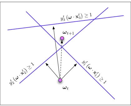
Figure 1: Illustration of the simultaneous projections algorithm: each instance casts a constraint on
ωand each such constraint defines a halfspace of feasible solutions. We project on each halfspace in parallel and the new vector is a weighted average of these projections
4. Simultaneous Projection Algorithms
Recall that on trial t the algorithm receives a matrix, Xt, of kt instances, and predicts ˆyt =Xtωt. After performing its prediction, the algorithm receives the corresponding labels yt. Each instance-label pair casts a constraint onωt, ytj
ωt·xt
j
≥1. If all the constraints are satisfied byωtthenωt+1 is set to beωt and the algorithm proceeds to the next trial. Otherwise, we would like to setωt+1as close as possible toωt while satisfying all constraints.
Such an aggressive approach may be sensitive to outliers and over-fitting. Thus, we allow some of the constraints to remain violated by introducing a trade-off between the change toωt and the loss attained on (Xt,yt). Formally, we would like to setωt+1 to be the solution of the following minimization problem,
min
ω∈Rn 1
2kω−ω
tk2+C`(ω;(Xt,yt)), (1) where C is a trade-off parameter. As we discuss below, this formalism effectively translates to a cap on the maximal change toωt. We rewrite the above optimization by introducing a single slack variable as follows:
min
ω∈Rn,ξ≥0 1 2
ω−ωt2+Cξ s.t. ∀j∈[kt]: ytj ω·xtj
≥1−ξ ξ≥0
. (2)
We denote the objective function of Eq. (2) by
P
t and refer to it as the instantaneous primal problem to be solved on trial t. The dual optimization problem ofP
t is the maximization problemmax
αt
1,..,αtkt kt
∑
j=1
αt
j− 1 2 ωt+
kt
∑
j=1
αt
jytjxtj 2
s.t. kt
∑
j=1
αt
j≤C , ∀j :αtj≥0 . (3)
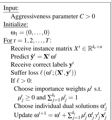
Input:
Aggressiveness parameter C>0 Initialize:
ω1= (0, . . . ,0) For t=1,2, . . . ,T :
Receive instance matrix Xt ∈Rkt×n Predict ˆyt=Xtωt
Receive correct labels yt Suffer loss`(ωt;(Xt,yt)) If` >0:
Choose importance weights µts.t. µtj≥0 and∑kt
j=1µtj=1
Choose individual dual solutionsαtj Updateωt+1=ωt+∑kt
j=1µtjαtjytjxtj
Figure 2: Template of simultaneous projections algorithm.
Each dual variable corresponds to a single constraint of the primal problem. The minimizer of the primal problem is calculated from the optimal dual solution as follows,ωt+1=ωt+∑kt
j=1αtjytjxtj. Unfortunately, in the common case, where each xtj is in an arbitrary orientation, there does not exist an analytic solution for the dual problem (Eq. 3). The difficulty stems from the fact that the sum of the weightsαt
jcannot exceed C. We tackle the problem by breaking it down into kt reduced problems, each of which focuses on a single dual variable. By doing so we replace the global sum constraint,∑kt
j=1αtj, with multiple box constraints,αtj≤C, which can easily be dealt with. Formally, for the j’th variable, the j’th reduced problem solves Eq. (3) while fixingαtj0=0 for all j06=j. Each
reduced optimization problem amounts to the following problem
max
αt j
αt
j− 1 2
ωt+αtjytjxtj2 s.t. αtj∈[0,C] . (4)
As we demonstrate in the sequel, this reduction into independent problems serves two roles. First, it leads to simple solutions for the reduced problems. Second, and more important, the individual solutions can and are grouped into a feasible solution of the original problem for which we can prove various loss bounds.
We thus next obtain an exact or approximate solution for each reduced problem as if it were independent of the rest. We then choose a non-negative vector µ∈∆kt where∆kt is the kt dimension probability simplex, formally µi ≥0 and ∑kjt=1µj =1. Given the vector µ, we multiply eachαtj by a corresponding value µtj. Our choice of µ assures us{µtjαtj}constitutes a feasible solution to the dual problem defined in Eq. (3) for the following reason. Each µtjαtj ≥0 and the fact that
αt
j ≤C implies that ∑ kt
j=1µtjαtj ≤C. Finally, the algorithm uses the combined solution and sets
ωt+1=ωt+∑kt
Variant Choosing µtj Choosingαtj
SimPerc ( 1
|Mt| j∈
M
t0 otherwise C
ConProj ( 1
|Mt| j∈
M
t0 otherwise min
C,`(ω
t;(xt j,ytj)) kxt
jk
2
ConProj ( 1
|Γt| j∈Γt
0 otherwise min
C,`(ω
t;(xt j,ytj)) kxt
jk
2
SimOpt See Fig. 4
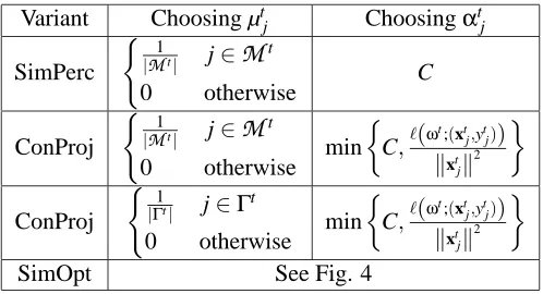
Figure 3: Schemes for choosing µ andα.
5. Solving the Reduced Problems
We next present four schemes to obtain a solution for the reduced problem (Eq. 4) and then combine the solution into a single update. The first three schemes provide feasible solutions for the reduced problems and are easy to implement. However, these solutions are not necessarily optimal. In Sec. 5.4 we describe a rather involved yet efficient procedure for finding the optimal solution of each reduced problem along side with their weight vector µ which constitute the means for combining the individual solutions.
5.1 Simultaneous Perceptron
The simplest of the update forms generalizes the famous Perceptron algorithm from Rosenblatt (1958) by settingαt
jto C if the j’th instance is incorrectly labeled, and to 0 otherwise. We then set the weight of µtj to |M1t| for j∈
M
t and to 0 otherwise. We abbreviate this scheme as the SimPerc algorithm.5.2 Soft Simultaneous Projections
The soft simultaneous projections scheme uses the fact that each reduced problem has an analytic
solution, which yieldsαtj=minC, `ωt;(xt j,ytj)
/ xtj
2
. We independently assign eachαtjthis
optimal solution. We next set µtjto be |Γ1t| for j∈Γt and to 0 otherwise. We would like to comment that this solution may updateαtj also for instances which were correctly classified as long as the margin they attain is not sufficiently large. We abbreviate this scheme as the SimProj algorithm.
5.3 Conservative Simultaneous Projections
Combining ideas from the above methods, the conservative simultaneous projections scheme opti-mally setsαtj according to the analytic solution. It differs from the SimProj algorithm in the way it selects µt. In the conservative scheme only the instances which were incorrectly predicted ( j∈
M
t) are assigned a positive weight. Put another way, µtjis set to 15.4 Jointly Optimizing µ andα
Recall that our goal is to propose a feasible solution to Eq. (3) and we do so by independently considering the optimization problem of Eq. (4) for each j. Following, we multiply eachαtj by a coefficient µtj so that all µtjαtj form a feasible solution. The following analysis shows that the two steps can be unified. For brevity, we omit the superscript t. The task of jointly optimizing both µ andαcasts a seemingly non-convex optimization and finding the optimal solution is a priori a hard problem. In this section we derive a somewhat counterintuitive result. By exploring the structure of the problem on hand we show that this joint optimization problem can efficiently be solved in ktlog kt time. .
We begin by taking the derivative of the optimal values forαjwhile assuming that the values µj are fixed and define a convex combination. The reduced problem of Eq. (4) becomes
max
αj
µjαj− 1 2
ω+µjαjyjxj 2 s.t. αj∈[0,C]
,
which can be rewritten as
max
αj
µjαj(1−yj(ω·xj))− 1 2µ
2 jα2j
xj
2−1
2kωk
2 s.t. α
j∈[0,C] .
For brevity, we denote the squared norm of xj byνj. Thus, omitting constants that do not depend onαjand µj, the above optimization problem can be written as
max
αj
µjαj(1−yj(ω·xj))− 1 2µ
2
jα2jνj s.t. 0≤αj≤C . (5) Let us denote the hinge-loss on instance j, max{0,1−yj(ω·xj)}by`j. By taking the derivative of the Lagrangian with respect toαj and equating the result with zero, we get that
αj=min
C, lj
µjνj
.
We can now look at two disjoint cases. The first case is when αj = lj
µjνj <C. In this caseαj takes the value of lj
µjνj and the value of the optimization problem above becomes
`2 j
νj−
1 2
`2 j
νj
=1
2 l2j
νj
.
We note in passing that this expression does not depend on µj.
The second case is whenαj=C. Pluggingαj into Eq. (5) we get the following expression, as a function of µ, which we denote by fj(µj),
fj(µj) =µjC`j− 1 2µ
2
jC2νj . (6)
We next take the derivative of fjabove with respect to µj and obtain
∂f
∂µj
from which we conclude that the optimal value for µj is
`j Cνj
.
Plugging the optimal value for µjback in Eq. (6) we get that the maximum of fj(µj)is
fj
`j Cνj
=`
2 j
νj−
1 2
`2 j
νj
=1
2
`2 j
νj
.
To recap, we may express the optimal value of Eq. (5) as a function of µjas follows.
fj(µj) =
µjC`j−12µ2jC2νj µj≤C`νjj 1
2
`2
j
νj otherwise
.
Thus, fj is monotonically increasing in the range 0≤µj≤ C`νjj and is constant for values greater than `j
Cνj.
Recall that our primary goal is to find a convex combination of µj. Thus, we would like to find the optimal assignment to µ given thatαis set optimally. We end up with the following optimization problem.
max
∑
jfj(µj)
s.t. ∀j : µj≥0
∑
jµj=1
. (7)
As previously discussed, for all j, fj increases in the range 0≤µj ≤C`νjj and is constant af-terwards. We may use this fact to further classify the structure of the optimal solution of Eq. (7). Assume first that∑j `j
Cνj ≤1. In this case we can increment each, µj=
`j
Cνj +B, where B is a non-negative constant which assures that∑jµj =1. This assignment of µ is clearly optimal, as fj is
increasing and reaches its maximum obtainable value for µj≥C`νjj. Now, suppose∑j `j
Cνj >1. In such a case there exists an optimal solution with µj≤
`j
Cνj for all j. Suppose in contrary that for every optimal solution µ there exists some ˆj where µˆj=C`νˆj
ˆj+εfor
some non-negativeε. Since ∑j `j
Cνj >1 there exists some j
0with µ j0 <C`νj0
j0. Since fj0 monotonely increases when µj0 < C`νj0
j0, while fˆj is constant for µˆj>
`ˆj
Cνˆj we can create a new assignment µ
?
increasing the value of the sum∑jfj(µj)by setting µ?ˆj=
`ˆj
Cνˆjand addεto µ?j0. We thus conclude that
for each solution where for some µˆj>C`νˆj
ˆj there exists an assignment µ
?where for all j, µ
j≤C`νjj and the objective of Eq. (7) is at least as high.
Thus, when∑j
`j
Cνj >1 we may add the constraint that µj ≤
`j
Cνj and obtain the following opti-mization problem.
max
µ
∑
j
fj(µj)
s.t. ∀j : 0≤µj≤
`j
Cνj
∑
j µj=1We next introduce non-negative Lagrange multipliers τ, {βj}, and {ηj} to obtain the following Lagrangian,
L=
∑
j
C`jµj− 1 2µ
2
jC2νj−
∑
jβjµj−τ
∑
j µj−1
!
+
∑
j
ηj
µj−
`j Cνj
.
Taking the derivative with respect to µjand comparing to 0 we get the following condition.
C`j−µjC2νj−βj−τ+ηj=0 , or
µj=
C`j−βj−τ+ηj C2ν
j
.
The complementary slackness assures us that when µj>0 thenβj=0 and thus
µj=
C`j−τ+ηj C2ν
j
.
Similarly, ηj >0 only when µj =C`νjj and is used only when τ is negative, However, τ may be negative only when∑j
`j
Cνj <1, which we covered before. To summarize, we can write the optimal solution as
µj=max{0,
C`j−τ C2ν
j }
. (8)
We now focus our attention on the task of finding the value of τ. First, note that every value ofτpartitions the set 1, . . . ,kt into two sets, indices j whose µj >0 and indices for which µj=0. Formally, let H =j|C`j>τ and L= [kt]\H denote the two sets partitioned according to τ. Clearly j∈H ⇐⇒ µj>0. Clearly, knowing the valueτallows us to compute the partition to H and L. The converse, however, is also true. Had we known H and L it would have been straightforward to computeτby using the fact that µ is in the probability simplex,∑jµj=1, to get that
∑
j∈H
C`j−τ C2ν
j
=1 . (9)
Eq. (9) allows us to easily computeτand obtain
τ=∑j∈H
C`j C2ν
j−1
∑j∈HC21ν
j
. (10)
In order to verifyτserve as a feasible solution, we’re required to verify that ∑j∈Hµj=1 and that for all j∈L : C`j−τ≤0. The following lemma states that there is only a single feasible value for
τ.
Input:
`j,νj j∈[kt] Algorithm:
Sort the indices{1, . . . ,kt}by decreasing order of`j For i=2, . . . ,kt:
Define H={1, . . . ,i−1}
Computeτ=∑j∈H
C`j C2νj−1
∑j∈HC21ν j
Validate C`i≤τ. If not, continue to next iteration Set µj=CC`2jν−τ
j Setαj=min n
C, lj µjνj
o
Figure 4: Calculating µ andαefficiently.
Proof Suppose by contradiction that there are two feasible values forτ, and denote these values as
τ1 andτ2. Denote H(τ1)and H(τ2)by H1and H2respectively. Assume without loss of generality thatτ1<τ2.
First we note that H2⊂H1. However, 1=
∑
j∈H1
C`j−τ1 C2ν
j
>
∑
j∈H1
C`j−τ2 C2ν
j
,
where the inequality is due to our assumption thatτ1<τ2. Since ∑j∈H2
C`j−τ2
C2ν
j must equal 1, we conclude that H2must strictly contain more items than H1. We have thus obtained a contradiction.
Using Lemma 1 we can devise an efficient algorithm for finding the optimal value for τ. We first sort the indices 1, . . . ,kt by decreasing order of `j. Then, for every i=2, . . . ,kt, we define Hi ={1, . . . ,i−1} and compute the value suitable value ofτ according to Eq. (10). Finally we verify if C`i≤τ. The algorithm for findingτis formally given in Fig. 4.
To recap, we have suggested a mechanism for jointly optimizing both µ andα. We showed that it suffices to find a valueτwhich consistently divides the set[kt]into two sets as follows. The first set corresponds to indices j for which µj is zero and the second includes the non-zero components of µ. Furthermore, we showed that onceτis known, obtaining the vector µ is a simple task. Last, we described how Lemma 1 translates into an efficient algorithm for finding τ. We thus derived another simultaneous projections scheme, denoted by SimOpt, which jointly optimized α and µ. This variant of the simultaneous projections framework is guaranteed to yield the largest increase in the dual compared to all other simultaneous projections schemes. We describe empirical results which validate experimentally this property in Sec. 9.
6. Analysis
bound on the number of trials on which the predictions of SimPerc and ConProj algorithms are imperfect. Following Shalev-Shwartz and Singer (2006a), the first step in the analysis is to tie the instantaneous dual problems to a global loss function. To do so, we introduce a primal optimization problem defined over the entire sequence of examples as follows,
min
ω∈Rn 1 2kωk
2+ C
T
∑
t=1
` ω; Xt,Yt .
We rewrite the optimization problem as the following equivalent constrained optimization problem,
min
ω∈Rn,ξ∈RT 1 2 kωk
2
+C
T
∑
t=1
ξt s.t. ∀t∈[T],∀j∈[kt]: ytj ω·xtj
≥1−ξt ∀t :ξt≥0 . (11)
We denote the value of the objective function at (ω,ξ)for this optimization problem by
P
(ω,ξ). A competitor who may see the entire sequence of examples in advance may in particular set(ω,ξ)to be the minimizer of the problem which we denote by (ω?,ξ?). Standard usage of Lagrange multipliers yields that the dual of Eq. (11) is,
max
λ
T
∑
t=1 kt
∑
j=1
λt,j−
1 2 T
∑
t=0 kt
∑
j=1
λt,jytjxtj 2
s.t. ∀t : kt
∑
j=1
λt,j≤C ∀t,j :λt,j≥0 . (12)
We denote the value of the objective function of Eq. (12) by
D
(λ1,···,λT), where eachλt is a vector inRkt. Through our derivation we use the fact that any set of dual variablesλ1,···,λT defines a feasible solutionω=∑tT=1∑kt
j=1λt,jytjxtjwith a corresponding assignment of the slack variables. Clearly, the optimization problem given by Eq. (12) depends on all the examples from the first trial through time step T and thus can only be solved in hindsight. We note however, that if we ensure thatλs,j=0 for all s>t then the dual function no longer depends on instances occurring on rounds proceeding round t. As we show next, we use this primal-dual view to derive the skeleton algorithm presented in Fig. 2 by finding a new feasible solution for the dual problem on every trial. Formally, the instantaneous dual problem, given by Eq. (3), is equivalent (after omitting an additive constant) to the following constrained optimization problem,
max
λ
D
(λ1,···,λt−1,λ,0,···,0) s.t. λ≥0 ,kt
∑
j=1
λj≤C . (13)
That is, the instantaneous dual problem is obtained from
D
(λ1,···,λT) by fixing λ1, . . . ,λt−1 to the values set in previous rounds, forcing λt+1 through λT to the zero vectors, and choosing a feasible vector forλt. Given the set of dual variablesλ1, . . . ,λt−1it is straightforward to show that the prediction vector used on trial t is ωt =∑ts−=11∑jλs,jysjxsj. Equipped with these relations and omitting constants which do not depend onλt, Eq. (13) can be rewritten as,max
λ1,...,λkt kt
∑
j=1
λj−
1 2
ωt+
∑
ktj=1
λjytjxtj 2
s.t. ∀j :λj≥0, kt
∑
j=1
λj≤C . (14)
The problems defined by Eq. (14) and Eq. (3) are equivalent. Thus, weighing the variables
αt
1, . . . ,αtkt by µ t
1, . . . ,µtkt also yields a feasible solution for the problem defined in Eq. (13), namely
Theorem 2 Let X1,y1, . . . , XT,yTbe a sequence of examples where Xt is a matrix of kt exam-ples and yt are the associated labels. Assume that for all t and j the norm of an instance xtj is at most R. Then, for anyω?∈Rnthe number of trials on which the prediction of SimPerc is imperfect is at most,
1 2kω
?k2+C∑T
t=1`(ω?;(Xt,yt)) C−12C2R2 .
Proof To prove the theorem we make use of the weak-duality theorem. Recall that any dual feasible
solution induces a value for the dual’s objective function which is upper bounded by the optimum value of the primal problem,
P
ω?,ξ?. In particular, the solution obtained at the end of trial T is dual feasible, and thusD
(λ1, . . . ,λT)≤P
(ω?,ξ?) .We now rewrite the left-hand side of the above equation as the following sum,D
(0, . . . ,0) +T
∑
t=1
D
(λ1, . . . ,λt,0, . . . ,0)−D
(λ1, . . . ,λt−1,0, . . . ,0).
Note that
D
(0, . . . ,0) equals 0. Therefore, denoting by∆t the difference in two consecutive dual objective values,D
(λ1, . . . ,λt,0, . . . ,0)−D
(λ1, . . . ,λt−1,0, . . . ,0), we get that∑Tt=1∆t≤P
(ω?,ξ?). We now turn to bounding ∆t from below. First, note that if the prediction on trial t is perfect (M
t =/0) then SimPerc setsλt to the zero vector and thus∆t =0. We can thus focus on trials for which the algorithm’s prediction is imperfect. We remind the reader that by unraveling the update ofωt we get thatωt =∑s<t∑ksj=1λs,jysjxsj. We now rewrite∆t as follows,
∆t =
kt
∑
j=1
λt,j−
1 2 ω
t+
∑
kt j=1λt,jytjxtj 2 +1 2
ωt2 . (15)
By construction,λt,j=µtjαtjand∑ kt
j=1µtj=1, which lets us further expand Eq. (15) and write,
∆t =
kt
∑
j=1
µtjαtj−1 2
ωt+
∑
ktj=1
µtjαtjytjxtj
2 +1 2 kt
∑
j=1
µtjωt2 .
The squared norm, k·k2is a convex function in its vector argument and thus∆t is concave, which yields the following lower bound on∆t,
∆t≥
kt
∑
j=1 µtj
αt j− 1 2
ωt+αtjytjxtj2+1
2 ωt2
. (16)
The SimPerc algorithm sets µtj to be 1/|
M
t|for all j∈M
t and to be 0 otherwise. Furthermore, for all j∈M
t,αtj is set to C. Thus, the right-hand side of Eq. (16) can be further simplified and written as,∆t≥
∑
j∈Mt µtj
C−1
2
ωt+Cytjxtj2+1
2 ωt2
.
Lemma 3 Letωt denote the predictor used by the SimPerc scheme on trial t. Let j∈
M
t denote an index of a mispredicted instance on trial t. Then1 2
ωt+Cytjxtj2−1 2
ωt2≤1 2C
2
ytjxtj2 .
Proof We start by expanding the norm of the vector after the update,
1 2
ωt+Cytjxtj2=1 2
ωt2+Cytjωt·xtj+1
2C 2
ytjxtj2 . Thus, the change in the norm is,
1 2
ωt+Cytjxtj2−1 2
ωt2 = 1
2
ωt2+Cytjωt·xtj+1
2C 2yt
jxtj 2−1
2 ωt2
= Cytjωt·xtj+1
2C 2
ytjxtj2 .
The set
M
t consists of indices of instances which were incorrectly classified. Thus, ytj(ωt·xtj)≤0for every j∈
M
t. The equation above can thus be further bounded by 12C2 ytjxtj2
.
Lemma 3 assures us that for all instances whose µj>0 the term12
ωt+Cytjxtj 2
−1 2kωtk
2 can be upper bounded. Therefore,∆t can further be bounded from below as follows,
∆t ≥
∑
j∈Mt µtj
C−1
2C 2
ytjxtj2
≥
∑
j∈Mt µtj
C−1
2C 2R2
=C−1
2C 2R2 ,
where for the second inequality we used the fact that the norm of all the instances is bounded by R. To recap, we have shown that on trials for which the prediction is imperfect∆t≥C−12C2R2, while in perfect trials where no mistake is made∆t=0. Putting all the inequalities together we obtain the following bound,
C−1
2C 2R2
ε≤
T
∑
t=1
∆t=
D
(λ1, . . . ,λT)≤P
(ω?,ξ?) ,whereεis the number of imperfect trials. Finally, rewriting
P
(ω?,ξ?)as1 2kω
?
k2+C T
∑
t=1
`(ω?;(Xt,yt) ,
yields the bound stated in the theorem.
Corollary 4 Under the same conditions of Thm. 2 and for anyω?∈Rn, the number of trials on which the prediction of either ConProj or SimOpt is imperfect is at most,
1
2kω?k2+C∑ T
t=1`(ω?;(Xt,yt)) C−12C2R2 .
Note that the predictions of the SimPerc algorithm do not depend on the specific value of C, thus for R=1 and an optimal choice of C the bound attained in Thm. 2 now becomes.
ε≤` ω?;(Xt,yt)+1
2kω
?k2+1 2
s
kω?k4+kω?k2 T
∑
t=1
`(ω?;(Xt,yt)) .
See Appendix B for a complete analysis.
We conclude this section with a few closing words about the SimProj variant. The SimPerc and ConProj algorithms ensure a minimal increase in the dual by focusing solely on classification errors and ignoring margin errors. While this approach ensures a sufficient increase of the dual, in practice it appears to be a double edged sword as the SimProj algorithm performs empirically better. This superior empirical performance can be motivated by a viewing the similarity of the update forms performed by the SimProj and SimOpt variants, which means that the actual increase in the dual attained by the SimProj algorithm is larger than can be guaranteed using worst case analysis.
7. Decomposable Losses
Recall that our algorithms tackle complex decision problems by decomposing each instance into multiple binary decision tasks, thus, on trial t the algorithm receives kt instances. The classifica-tion scheme is evaluated by looking at the maximal violaclassifica-tion of the margin constraints`(ˆyt,yt) =
maxj h
1−ytjyˆtji
+. While such approach often captures the inherent relation between the multiple
binary tasks, it may often be desired to introduce more complex evaluation measures. In this section we introduce a generalization of the algorithm for various decomposable losses. As a corollary we obtain a Simultaneous Projection algorithm that is competitive with the average performance error on each set of kt instances.
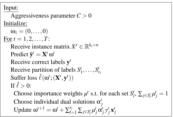
First, we introduce the notion of the decomposable losses. On trial t the algorithms receives a partition of the kt instances into rt sets. Let St1, . . . ,Srtt denote a partition of[kt]into rt sets, namely, ∪lStl= [kt]and∀l=6 k : Stl∩Stk=/0. A set Slties the instances in the sense that failing to predict any instance in Sl amounts to the same error as failing to predict all of them. We thus suffer a unit loss at trial t for each set Sl that was imperfectly predicted. The definition of the loss is extended to
ˆ
` ˆyt,yt= 1
rt rt
∑
l=1 max
j∈Stl
1−ytjyˆtj
+ . (17)
By construction, the setting suggested in Sec. 2 is a special case of the setting we consider in this section. We show in the sequel though that our original analysis carries over this this more general setting.
Input:
Aggressiveness parameter C>0 Initialize:
ω1= (0, . . . ,0) For t=1,2, . . . ,T :
Receive instance matrix Xt ∈Rkt×n Predict ˆyt=Xtωt
Receive correct labels yt
Receive partition of labels St1, . . . ,Strt Suffer loss ˆ`(ωt;(Xt,yt))
If ˆ` >0:
Choose importance weights µt s.t. for each set Stl,∑j∈St lµ
t j=1 Choose individual dual solutionsαtj
Updateωt+1=ωt+∑rt
l=1∑j∈Stlµ t
jαtjytjxtj
Figure 5: The extended simultaneous projections algorithm for decomposable losses.
each set as follows:
min
ω∈Rn,ξ≥0 1 2
ω−ωt2+C rt
rt
∑
l=1
ξl
s.t. ∀l∈[rt], ∀j∈Stl: ytj ω·xtj
≥1−ξl ∀l∈[rt]: ξl≥0
. (18)
The dual of Eq. (18) is thus
max
αt
1,..,αtkt kt
∑
j=1
αt
j− 1 2 ωt+
kt
∑
j=1
αt
jytjxtj 2
s.t. ∀l :
∑
j∈St lαt
j≤ C rt ∀
j :αtj≥0
.
Note that since∀k6=l : Stl∩Stk= /0then the induced constraint ∑j∈St lα
t
j≤ Crt corresponds to a unique set of dual variablesαtj. We can thus apply the same technique and select a non-negative vector µ where the entries corresponding to each set Stl form a probability distribution, namely ∀l :∑j∈St
lµ t
j =1. To recap, we can employ any of the variants on each set separately and attain a dual feasible solution. We denote these variants as the decomposition variants. In Fig. 5 we provide the pseudo-code of the algorithm.
We next show that our mistake bound analysis can be extended to the decomposable loss. The analysis follows closely to the analysis presented in Sec. 6, where the global primal and global dual are modified so as to use the decomposition loss. We therefore focus only on highlighting the necessary changes. Eq. (11) thus becomes
min
ω∈Rn,ξ∈RT 1 2 kωk
2
+C
T
∑
t=1 rt
∑
l=1
ξt,l rt
s.t. ∀t∈[T],∀l∈[rt],∀j∈Stl: ytj ω·xtj
≥1−ξt,l ∀t∀l :ξt,l ≥0
and its dual is
max
λ
T
∑
t=1 kt
∑
j=1
λt,j−
1 2
T
∑
t=0 kt
∑
j=1
λt,jytjxtj 2
s.t. ∀t∀l∈[rt]:
∑
j∈St lλt,j≤
C rt ∀
t,j :λt,j≥0 .
Clearly, the instantaneous dual can still be seen as optimizing the global dual, while fixing the dual variablesλt0,j for all t06=t.
To recap, we replace the loss of the instantaneous optimization problem defined in Eq. (1) with the average over a decomposition of losses ˆ`as defined by Eq. (17). Next, in order to obtain a mistake bound, we look at the global optimization task defined by Eq. (19). As previously showed, the simultaneous projection scheme can be viewed as an incremental update to the dual of Eq. (19). It is interesting to note that for every decomposition of the kt instances into sets, the value of
ˆ
`(ω;(Xt,yt))is upper bounded by`(ω;(Xt,yt)), as ˆ`is the average over the margin violations while
`corresponds to the worst margin violation. Thus, the loss underpinning the global optimization from Eq. (11) upper bounds the loss yielding Eq. (19). The following corollary immediately holds.
Corollary 5 Under the same conditions of Thm. 2, the loss suffered along the run of either
decom-position variant is at most, 1 2kω
?k2+C∑T
t=1`ˆ(ω?;(Xt,yt)) C−12C2R2 .
In conclusion, the simultaneous projection scheme allows us to easily obtain online algorithms and update schemes for complex problems, such algorithms are obtained by decomposing a complex problem into multiple binary problems. It is often the case where the maximal violation over all binary problems correctly captures the inherent violation of the original complex problem. In this section we explored cases where a more refined definition of error is required. Specifically, if we define each binary instance in a separate set, we obtain an algorithmic framework where our competitor is evaluated according to the average loss.
8. Simultaneous Multiplicative Updates
In this section we describe and analyze a multiplicative version of the simultaneous projection scheme. Recall that our motivation was to introduce a solution to the instantaneous optimization problem given in Eq. (2). The instantaneous objective captures the following trade-off. On one hand we would like to setωto be as close as possible toωt. On the other hand, we would like to minimize the loss incurred by the instances received on trial t. In previous sections we used the squared Euclidean norm to define the measure of distance betweenωt andω. In this section we take a different approach and use the relative entropy as the notion of closeness between two vectors. By doing so we derive a multiplicative version of our online algorithmic framework. In this section we confine ourselves to linear predictors that lie in the probability simplex, that is, we consider non-negative vectorsωsuch that∑ni=1ωi=1. Previously, we used a fixed value of 1 for the margin that is needed in order to suffer no loss, where it was understood that we may simultaneously scale the prediction vector and the margin. Since we now prevent such scaling due to the choice of the simplex domain, we need to slightly modify the definition of the loss and introduce the following definition,`γ(ˆyt,yt) =maxj
h
γ−ytjyˆtji
Recall that on trial t the algorithm receives kt instances arranged in a matrix Xt. After extending a prediction vector,ωtXt, the algorithm receives the vector of correct labels yt and suffers a loss for any incorrect prediction. If no mistake is made the algorithm proceeds to the next round. Otherwise we would like to setωtto be the solution of the following optimization problem
min
ω∈∆n
DKL(ωkωt) +C`γ(ω;(Xt,yt)) , (20) where C is a trade-off parameter. The term DKL is the relative entropy operator, also known as the Kullback-Leibler divergence, and is defined as
DKL ωkωt=
n
∑
i=1
ωilogωωti
i
.
The dual problem of Eq. (20) is,
γ
∑
ktj=1
αt
j−log n
∑
i=1
ωt
iexp kt
∑
j=1
τj
i !!
s.t.
kt
∑
j=1
αt
j≤C ∀j :αtj≥0 ∀j :τj=αtjytjxtj
. (21)
The prediction vectorωis set as follows,
ωi=ωti
exp
∑kt j=1τ
j i
∑n
l=1ωtlexp
∑kt
j=1τ j i
. (22)
The complete derivation of the dual problem and the update ofωis given in Appendix A.
We follow the same technique suggested in Sec. 4 and decompose Eq. (21) into kt separate problems, each concerning a single dual variable. The resulting j’th reduced dual problem is thus
γαt
j−log n
∑
i=1
ωt
iexp
τj
i !
s.t. 0≤αtj≤C τj=αt jytjxtj
. (23)
We next obtain an exact or approximate solution for each reduced problem as if it were independent of the rest. We follow by choosing a vector µ∈∆kt, and multiply each α
t
j by a corresponding value µtj. Our choice of µ assures us {µtjαtj} constitutes a feasible solution to the dual problem defined in Eq. (21) for the following reason. Each µtjαtj≥0 and the fact thatαtj≤C implies that
∑kt
j=1µtjαtj ≤C. Finally, the algorithm uses the combined solution and setsωt+1 according to Eq. (22). The template of the multiplicative simultaneous projections algorithm is described in Fig. 6.
We may now apply the methods introduced in Sec. 5 and introduce the multiplicative schemes. The SimPerc scheme can be trivially applied to the multiplicative setting. We next show a closed-form solution toαtjfor each reduced problem if the components of each instance are from{−1,0,1}n. To so we need to introduce the following notation.
Wj+=
∑
i:ytjxtji=1
ωt
i
n
∑
l=1
ωt
l
,Wj−=
∑
i:ytjxtji=−1
ωt
i
n
∑
l=1
ωt
l
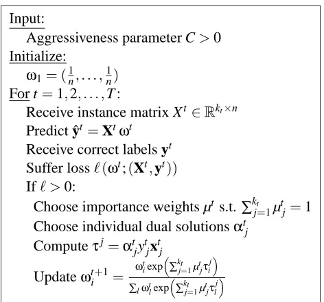
Input:
Aggressiveness parameter C>0 Initialize:
ω1= (1n, . . . ,1n) For t=1,2, . . . ,T :
Receive instance matrix Xt∈Rkt×n Predict ˆyt =Xtωt
Receive correct labels yt Suffer loss`(ωt;(Xt,yt)) If` >0:
Choose importance weights µt s.t.∑kt
j=1µtj=1 Choose individual dual solutionsαtj
Computeτj=αt jytjxtj
Updateωti+1= ω
t iexp
∑kt j=1µtjτ
j i
∑lωtlexp
∑kt j=1µtjτ
j l
Figure 6: The multiplicative simultaneous projections algorithm.
The optimal value ofαtj is thus log of the root of a quadric equation with Wj+, Wj−, Wj0as coeffi-cients. We also need to take into account the boundary constraints onαt
j, namely, 0≤αtj≤C. Thus,
αt
j is the minimum between the following root and C,
log
γW0
j + q
γ2(W0
j)2+4(1−γ2)Wj+Wj− 2(1−γ)Wj+
,
The derivation can be found at Appendix C. Using the closed-form solution forαtj we can adapt both the ConProj and SimProj scheme to the multiplicative setting.
We next turn our attention to the analysis of the multiplicative algorithm and focus on the Sim-Perc scheme. The analysis here follows closely the analysis presented in Sec. 6. Hence, the remain-der of this section focuses on highlighting the key changes that are required. Formally, we prove the following theorem.
Theorem 6 Let X1,y1, . . . , XT,yTbe a sequence of examples where Xt is a matrix of kt exam-ples and yt are the associated labels. Assume that for all t and j the`∞norm of an instance xtjis at most R. Then, for anyω?∈∆nthe number of trials on which the prediction of SimPerc is imperfect is at most,
∑n
i=1ω?i log
ω?
i 1/n+C∑
T
t=1`γ(ω?;(Xt,yt)) C−12C2R2 .
Proof Following the technique introduced in Sec. 6, our goal is to upper bound the number of
Our competitor is thus evaluated using the global optimization problem given by,
min
ω∈∆n,ξ≥0 n
∑
i=1
ωilog
ωi ωt i +C T
∑
t=1
ξt
s.t. ∀t∈[T],∀j∈[kt]: ytj ω·xtj
≥γ−ξt ∀t :ξt ≥0
. (24)
The dual of Eq. (24) is
γ
∑
Tt=1 kt
∑
j=1
λt j−log
n
∑
i=1 exp
T
∑
t=1 kt
∑
j=1
τt j i
!!
s.t. ∀t∈[T]: kt
∑
j=1
λt
j≤C ∀t,∀:λtj≥0 ∀t,∀j :τt j=λtjytjxtj
. (25)
We denote the objective of Eq. (25) by
D
(λ1, . . . ,λT). The instantaneous dual of Eq. (21) can be seen as incrementally building an assignment for the dual: At trial t we fixλs for s<t to their previous values, and fixλsfor s>t to 0. Thusωt is defined as followsωt
i= exp
∑t
s=1∑ ks
j=1τ s j i
∑n
l=1exp
∑T
s=1∑ ks
j=1τ s j l
.
The key difference between the multiplicative schemes and the previously analyzed scheme lies in Lemma 3. We thus progress to derive a similar lemma for the multiplicative setting.
Lemma 7 Letθ=∑tl−=11∑kl
j=1λtjytjxtj denote the dual variables assigned in trials prior to t by the SimPerc scheme. Let j∈
M
t denote an index of a mispredicted instance on trial t. Then, the difference,log n
∑
i=1
exp θi+Cxtjiytj
!
−log n
∑
i=1
exp(θi) !
,
is upper bounded by 12C2kxk2∞.
Proof Denote the vector Cxtjytjbyτ. Let F(θ)denote the value of log ∑ni=1eθi. Hence, we would like to upper bound the difference F(θ+τ)−F(θ). We prove the lemma based on the following inequality
F(θ+τ)−F(θ) ≤ n
∑
i=1 eθi
∑leθl
τi+
1 2maxi τ
2 i .
The above inequality was used and proved in numerous previous analyses of multiplicative update methods. See for instance Examples 2 and 5 in Kivinen and Warmuth (2001). Consider the term
∑n
i=1 e
θi
∑leθlτi. Recall that the prediction in trial t is made by using the predictor defined by Eq. (22). Thus, the above term is the following inner product between the vectorτand the predictor used on round t,
n
∑
i=1 eθi
∑leθl
τi=
n
∑
i=1
ωt
where the last inequality is due to the fact that we assume j∈
M
t (the prediction was incorrect) and the inner-product is non-positive. Therefore, we obtain the required upper boundF(θ+τ)−F(θ)≤1 2maxi τ
2 i
1 2kτk
2
∞= 12C2xtj2∞ .
To recap, we showed that the instantaneous dual can be seen as incrementally constructing an assignment for a global dual function (Eq. 25). Furthermore, we showed that Lemma 3 can be adapted to the multiplicative settings. The rest of the proof follows the same lines of the proof given in Sec. 6. Namely, trials in which a prediction mistake was made, the SimPerc scheme is guaranteed a substantial increase in the incremental dual buildup. Finally, using weak-duality we obtain that the evaluation measure for the competitor is the lower bounded by,
∑n
i=1ω?i log
ω?
i 1/n+C∑
T
t=1`γ(ω?;(Xt,yt)) C−12C2R2 .
The multiplicative ConProj scheme assigns αtj the value which maximizes the reduced instan-taneous dual. The ConProj scheme thus maximizes the difference between the value of the global dual in two consecutive rounds. We thus obtain an equivalent corollary of Corollary 4 for the mul-tiplicative setting.
Corollary 8 Under the same conditions of Thm. 6 and for anyω?∈Rn, the number of trials on which the prediction of the ConProj scheme is imperfect is at most,
∑n
i=1ω?i log
ω?
i 1/n+C∑
T
t=1`γ(ω?;(Xt,yt)) C−12C2R2 .
We thus showed that the multiplicative SimPerc and ConProj schemes entertain a similar mis-take bound as the original formulation. Note, however, that in the multiplicative settings we assume that the`∞norm of all instances are bounded by R, while in the additive settings, we have assumed that the`2norm of the instances is bounded by R.
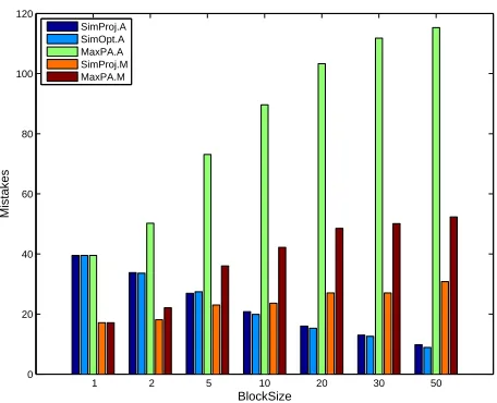
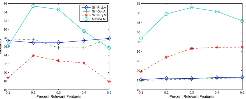
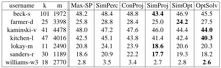
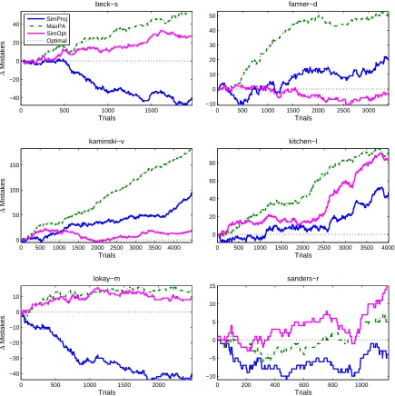
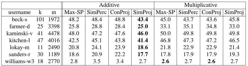
9. Experiments