Cautious Collective Classification
Luke K. McDowell [email protected]
Department of Computer Science U.S. Naval Academy
Annapolis, MD 21402, USA
Kalyan Moy Gupta [email protected]
Knexus Research Corporation Springfield, VA 22153, USA
David W. Aha [email protected]
Navy Center for Applied Research in Artificial Intelligence Naval Research Laboratory (Code 5514)
Washington, DC 20375, USA
Editor: Michael Collins
Abstract
Many collective classification (CC) algorithms have been shown to increase accuracy when in-stances are interrelated. However, CC algorithms must be carefully applied because their use of estimated labels can in some cases decrease accuracy. In this article, we show that managing this label uncertainty through cautious algorithmic behavior is essential to achieving maximal, robust performance. First, we describe cautious inference and explain how four well-known families of CC algorithms can be parameterized to use varying degrees of such caution. Second, we introduce
cautious learning and show how it can be used to improve the performance of almost any CC
al-gorithm, with or without cautious inference. We then evaluate cautious inference and learning for the four collective inference families, with three local classifiers and a range of both synthetic and real-world data. We find that cautious learning and cautious inference typically outperform less cautious approaches. In addition, we identify the data characteristics that predict more substantial performance differences. Our results reveal that the degree of caution used usually has a larger
im-pact on performance than the choice of the underlying inference algorithm. Together, these results
identify the most appropriate CC algorithms to use for particular task characteristics and explain multiple conflicting findings from prior CC research.
Keywords: collective inference, statistical relational learning, approximate probabilistic infer-ence, networked data, cautious inference
1. Introduction
Collective classification (CC) is a method for jointly classifying related instances. To do so, CC methods employ a collective inference algorithm that exploits dependencies between instances (e.g., autocorrelation), enabling CC to often attain higher accuracies than traditional methods when instances are interrelated (Neville and Jensen, 2000; Taskar et al., 2002; Jensen et al., 2004; Sen et al., 2008). Several algorithms have been used for collective inference, including relaxation label-ing (Chakrabarti et al., 1998), the iterative classification algorithm (ICA) (Lu and Getoor, 2003a), loopy belief propagation (LBP) (Taskar et al., 2002), Gibbs sampling (Gibbs) (Jensen et al., 2004), and variants of the weighted-vote relational neighbor algorithm (wvRN) (Macskassy and Provost, 2007).
During testing, all collective inference algorithms exploit relational features based on uncertain estimation of class labels. This test-time label uncertainty can diminish accuracy due to two related effects. First, an incorrectly predicted label during testing may negatively influence the predictions of its linked neighbors, possibly leading to cascading inference errors (cf., Neville and Jensen, 2008). Second, the training process may learn a poor model for test-time inference, because of the disparity between the training scenario (where labels are known and certain) and the test scenario (where labels are estimated and hence possibly incorrect). As a result, while CC has many potential advantages, in some cases CC’s label uncertainty may actually cause accuracy to decrease compared to non-relational approaches (Neville and Jensen, 2007; Sen and Getoor, 2006; Sen et al., 2008).
In this article, we argue that managing this test-time label uncertainty through “cautious” al-gorithmic behavior is essential to achieving maximal, robust performance. We describe two com-plementary cautious strategies. Each addresses the fundamental problem of label uncertainty, but separately targets the two manifestations of the problem described above. First, cautious
infer-ence is an inferinfer-ence process that attends to the uncertainty of its intermediate label predictions.
For example, existing algorithms such as Gibbs or LBP accomplish cautious inference by sampling from or directly reasoning with the estimated label distributions. These techniques are cautious because they prevent less certain label estimates from having substantial influence on subsequent estimations. Alternatively, we show how variants of a simpler algorithm, ICA, can perform cautious inference by appropriately favoring more certain information. Second, cautious learning refers to a training process that ameliorates the aforementioned train/test disparity. In particular, we introduce PLUL (Parameter Learning for Uncertain Labels), which uses standard cross-validation techniques, but in a way that is new for CC and that leads to significant performance advantages. In particu-lar, PLUL is cautious because it prevents the algorithm from learning a model from the (correctly labeled) training set that overestimates how useful relational features will be when computed with uncertain labels from the test set.
We consider four frequently-studied families of CC algorithms: ICA, Gibbs, LBP, and wvRN. For each family, we describe algorithms that use varying degrees of cautious inference and explain how they all (except for the relational-only wvRN) can also exploit cautious learning via PLUL. We then evaluate the variants of these four families, with and without PLUL, over a wide range of synthetic and real-world data sets. To broaden the evidence for our results, we evaluate three local classifiers that are used by some of the CC algorithms, and also compare against a non-relational baseline.
While recent CC studies describe complementary results and make some related comparisons, they omit important variations that we consider here (see Section 3). Moreover, the scope and/or methodology of previous studies leaves several important questions unanswered. For instance,
to work well for CC (Jensen et al., 2004; Neville and Jensen, 2007). If so, why did Sen et al. (2008) find no significant difference between Gibbs and the much less sophisticated ICA? Second,
we earlier reported that ICAC(a cautious variant of ICA) outperforms both Gibbs and ICA on three
real-world data sets (McDowell et al., 2007a). Why would ICACoutperform Gibbs, and for what
data characteristics are ICAC’s gains significant? We answer these questions and more in Section 8.
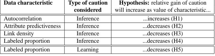
We hypothesize that cautious CC algorithms will outperform more aggressive CC approaches
when there exists a high probability of an “incorrect relational inference”, which we define as a
pre-diction error that is due to reasoning with relational features (i.e., an error that does not occur when relational features are removed). Two kinds of data characteristics increase the likelihood of such errors. First, when the data characteristics lead to lower overall classification accuracy (e.g., when the non-relational attributes are not highly predictive), then the computed relational feature values will be less reliable. Second, when a typical relational link is highly predictive (e.g., as occurs when the data exhibits high relational autocorrelation), then the potential effect of any incorrect predic-tion is magnified. As the magnitude of either of these data set characteristics increases, cautious algorithms should outperform more aggressive algorithms by an increasing amount.
Our contributions are as follows. First, we describe cautious inference and how four commonly-used families of existing CC inference algorithms can exhibit more or less caution. Second, we introduce cautious learning and explain how it can help compensate for the train/test disparity that occurs when a CC algorithm uses estimated class labels during testing. Third, we identify the data characteristics for which these cautious techniques should outperform more aggressive approaches, as introduced in the preceding paragraph and discussed in more detail in Section 6. Our experi-mental results confirm that cautious approaches typically do outperform less cautious variants, and that these effects grow larger when there is a greater probability of incorrect relational inference. Moreover, our results reveal that in most cases the degree of caution used has a larger impact on
performance than the choice of the underlying inference algorithm. In particular, the cautious
algo-rithms perform very similarly, regardless of whether ICAC or Gibbs or LBP is used, although our
results also confirm that, for some data characteristics, inference with LBP performs comparatively poorly. These results suggest that in many cases the higher computational complexity of Gibbs and
LBP is unnecessary, and that the much faster ICACshould be used instead. Finally, our results and
analysis enable us to answer the previously mentioned questions regarding CC.
The next two sections summarize collective classification and related work. Section 4 then explains why CC needs to be cautious and describes cautious inference and learning in more detail. In Section 5, we describe how caution can be specifically used by the four families of CC inference algorithms. Section 6 then describes our methodology and hypotheses. Section 7 presents our results, which we discuss in Section 8. We conclude in Section 9.
2. Collective Classification: Description and Problem Definition
In this section, we first motivate and define collective classification (CC). We then describe different approaches to CC, different CC tasks, and our assumptions for this article.
2.1 Problem Statement and Example
as predicting the topic of a publication or the group membership of a person (Koller et al., 2007). More formally, we consider the following task (based on Macskassy and Provost, 2006):
Definition 1 (Classification of Graph-based Data) Assume we are given a graph G= (V,E,X,Y,C)
where V is a set of nodes, E is set of (possibly directed) edges, each~xi∈X is an attribute vector for
node vi∈V , each Yi∈Y is a label variable for vi, and C is the set of possible labels. Assume further
that we are given a set of “known” values YKfor nodes VK⊂V , so that YK={yi|vi∈VK}. Then the
task is to infer YU, the values of Yifor the remaining nodes with “unknown” values (VU=V−VK),
or a probability distribution over those values.1
For example, consider the task of predicting whether a web page belongs to a professor or a stu-dent. Conventional supervised learning approaches ignore the link relations and classify each page using attributes derived from its content (e.g., words present in the page). We refer to this approach as non-relational classification. In contrast, a technique for relational classification would explicitly use the links to construct additional relational features for classification (e.g., for each page, includ-ing as features the words from hyperlinked pages). This additional information can potentially in-crease classification accuracy, though may sometimes dein-crease accuracy as well (Chakrabarti et al., 1998). Alternatively, even greater (and usually more reliable) increases can occur when the class
labels of the linked pages are used instead to derive relevant relational features (Jensen et al., 2004).
However, using features based on these labels is challenging, because some or all of the labels are initially unknown, and thus typically must be estimated and then iteratively refined in some way. This process of jointly inferring the labels of interrelated nodes is known as collective classification (CC).
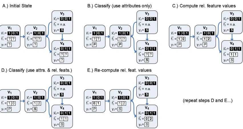
Figure 1 summarizes an example execution of a simple CC algorithm, ICA, applied to the binary web page classification task. Each step in the sequence displays a graph of four nodes, where each
node denotes a web page, and hyperlinks among them. Each node has a class label yi; the set of
possible class labels is C={P,S}, denoting professors and students, respectively. Three nodes have
unknown labels (VU={v1,v2,v4}) and one node has a known label (VK={v3}). In the initial state
(step A), no label yihas yet been estimated for the nodes in VU, so each is set to missing (indicated
by a question mark). Each node has three binary attributes (represented by~xi). Nodes in VU also
have two relational features (one per class), represented by the vector~fi. Each feature denotes the
number of linked nodes (ignoring link direction) that have a particular class label.
In step B, some classifier (not shown) estimates class labels for nodes in VUusing only the
(non-relational) attributes. These labels, along with the known label y3, are used in step C to compute
the relational feature value vectors. For instance, in step C, ~f2= (1 2) because v2 links to nodes
with one current P label and two current S labels. In step D, a classifier re-estimates the labels using both attributes and relational features, which changes the predicted label of v2. In step E, relational
feature values are re-computed using the new labels. Steps D and E then repeat until a termination criterion is satisfied (e.g., convergence, number of iterations).
This example exhibits how relational value uncertainty occurs with CC. For instance, the feature vector~f1 is(1 0)in step C but later becomes(0 1). Thus, intermediate predictions use uncertain
label estimates, motivating the need to cautiously use such estimates.
!""#$%&" ' (& ")$
* *
! !)+,& ' # &'- &"
. / . 0
1 ! ""#$%&" '" 2' # "
3 4 . 3 5 3 3 0
6 7 8 9) +,&' # - &"
. 3 5 0 / 0
%' , " ,"1:6
Figure 1: Example operation of ICA, a simple CC algorithm. Each step (A thru E) shows a graph of 4 linked nodes (i.e., web pages). “Known” values are are shown in white text on a black background; this includes all attribute values~xi and the class label y3 for v3. Estimated
values are shown instead with a white background.
2.2 Algorithms for Collective Inference
For some collective inference tasks, exact methods such as junction trees (Huang and Darwiche, 1996) or variable elimination (Zhang and Poole, 1996) can be applied. However, these methods may be prohibitively expensive to use (e.g., summing over the remaining variable configurations is intractable for modest-sized graphs). Some research has focused on methods that further factorize the variables, and then apply an exact procedure such as belief propagation (Neville and Jensen, 2005), min-cut partition (Barzilay and Lapata, 2005), or methods for solving quadratic and linear programs (Triebel et al., 2007). In this article, we consider only approximate collective inference methods.
We consider three primary types of approximate collective inference algorithms, borrowing some terminology from Sen et al. (2008):
• Local classifier-based methods. For these methods, inference is an iterative process whereby
• Global formulation-based methods. These methods train a classifier that seeks to
opti-mize one global objective function, often based on a Markov random field (Dobrushin, 1968; Besag, 1974). As above, the classifier uses both attributes and relational features for infer-ence. Examples of these algorithms include loopy belief propagation and relaxation labeling. These do not use a separate local classifier; instead, the entire algorithm is used for both train-ing (e.g., to learn the clique potentials) and inference. See Taskar et al. (2002) and Sen et al. (2008) for more details.
• Relational-only methods. Recently, Macskassy and Provost (2007) demonstrated that, when
some labels are known (i.e.,|VK|>0), algorithms that use only relational information can in some cases perform very well. We consider several variants of the algorithm they described,
wvRNRL(weighted-vote relational neighbor, with relaxation labeling). This algorithm
com-putes a new label distribution for a node by averaging the current distributions of its neighbors. It does not require any training.
With local classifier methods, learning the classifier can often be done in a single pass over the data, does not require running collective inference, and in fact is independent of the collective infer-ence procedure that will be used. In contrast, for global methods the local classifier and inferinfer-ence algorithm are effectively unified. As a result, learning for a global method requires committing to and actually executing a specific inference algorithm, and thus can be much slower than with a local classifier-based method.
All of these algorithms jointly classify interrelated nodes using some iterative process. Those that propagate from one iteration to the next a single label for each node are called hard-labeling methods. Methods that instead propagate a probability distribution over the possible class labels are called soft-labeling methods (cf., Galstyan and Cohen, 2007). All of the local classifier-based
methods that we examine are hard-labeling methods.2 Soft-labeling methods, such as variants of
relaxation labeling, are also possible but require that the local classifier be able to reason directly with label distributions, which is more complex than the label aggregation for features typically done with approaches like ICA or Gibbs. Section 6.6 provides more detail on these features.
2.3 Task Definitions and Focus
Collective classification has been applied to two types of inference tasks, namely the out-of-sample
task, where VK is empty, and the in-sample task, where VK is not empty. Both types of tasks
may emerge in real-world situations (Neville and Jensen, 2005). Prior work on out-of-sample tasks (Neville and Jensen, 2000; Taskar et al., 2002; Sen and Getoor, 2006) assume that the algorithm is
also provided with a training graph GTrthat is disjoint from the test graph G. For instance, a model
may be learned over the web-graph for one institution, and tested on the web-graph of another. For in-sample tasks, where some labels in G are known, CC can be applied to the single graph
G (Macskassy and Provost, 2007; McDowell et al., 2007a; Sen et al., 2008; Gallagher et al., 2008); within-network classification (Macskassy and Provost, 2006) involves training on the subset GK⊂G
with known labels, and testing by running inference over the entire graph. This task simulates, for example, fraud detection in a single large telecommunication network where some entities/nodes are
2. We could also consider wvRNRL, which is a soft-labeling method, to be a local classifier-based method, albeit a
known to be fraudulent. Another in-sample task (Neville and Jensen, 2007; Bilgic and Getoor, 2008;
Neville and Jensen, 2008) assumes a separate training graph GTr, where a model is learned from
GTr and inference is performed over the test graph G, which includes both labeled and unlabeled
nodes. For both tasks, predictive accuracy is measured only for the unlabeled nodes.
In Section 6, we will address three types of tasks (i.e., out-of-sample, sparse in-sample, and dense in-sample). This is similar to the set of tasks addressed in some previous evaluations (e.g., Neville and Jensen, 2007, 2008; Bilgic and Getoor, 2008) and subsumes some others (e.g., Neville and Jensen, 2000; Taskar et al., 2002; Sen and Getoor, 2006). We will not directly address the within-network task, but the algorithmic trends observed from our in-sample evaluations should be similar.3
2.4 Assumptions and Limitations
In this broad investigation on the utility of caution in collective classification, we make several simplifying assumptions. First, we assume data is obtained passively rather than actively (Rattigan et al., 2007; Bilgic and Getoor, 2008). Second, we assume that nodes are homogeneous (e.g., all represent the same kind of object) rather than heterogeneous (Neville et al., 2003a; Neville and Jensen, 2007). Third, we assume that links are not missing, and need not be inferred (Bilgic and Getoor, 2008). Finally, we do not attempt to increase autocorrelation via techniques such as link addition (Gallagher et al., 2008), clustering (Neville and Jensen, 2005), or problem transformation (Tian et al., 2006; Triebel et al., 2007).
Our example in Figure 1 employs a simple relational feature (i.e., that counts the number of linked nodes with a specific class label). However, several other types of relations exist. For ex-ample, Gallagher and Eliassi-Rad (2008) describe a topology of feature types, including structural features that are independent of node labels (e.g., the number of linked neighbors of a given node). We focus on only three simple types of relational features (see Section 6.6), and leave broader in-vestigations for future work. Likewise, for CC algorithms that learn, we assume that training is performed just once, which differs from some prior work where the learned model is updated in each iteration (Lu and Getoor, 2003b; Gurel and Kersting, 2005).
3. Related Work
Besag (1986) originally described the “Iterated Conditional Modes” (ICM) algorithm, which is a version of the ICA algorithm that we consider. Several researchers have reported that employ-ing inter-instance relations in CC algorithms can significantly increase predictive accuracy (e.g., Chakrabarti et al., 1998; Neville and Jensen, 2000; Taskar et al., 2002; Lu and Getoor, 2003a). Furthermore, these algorithms have performed well on a variety of tasks, such as identifying secu-rities fraud (Neville et al., 2005), ranking suspicious entities (Macskassy and Provost, 2005), and annotating semantic web services (Heß and Kushmerick, 2004).
In each iteration, a CC algorithm predicts a class label (or a class distribution) for each node and uses it to determine the next iteration’s predictions. Although using label predictions from linked nodes (instead of using the larger number of attributes from linked nodes) encapsulates the influence of a linked node and simplifies learning (Jensen et al., 2004), it can be problematic. For example,
iterating with incorrectly predicted labels can propagate and amplify errors (Neville and Jensen, 2007; Sen and Getoor, 2006; Sen et al., 2008), diminishing or even reducing accuracy compared to non-relational approaches. In this article, we examine the data characteristics (and algorithmic interactions) for which these issues are most serious and explain how cautious approaches can ame-liorate them.
The performance of CC compared to non-relational learners depends greatly on the data char-acteristics. First, for CC to improve performance, the data must exhibit relational autocorrelation (Jensen et al., 2004; Neville and Jensen, 2005; Macskassy and Provost, 2007; Rattigan et al., 2007; Sen et al., 2008), which is correlation among the labels of related instances (Jensen and Neville, 2002). Complex correlations can be exploited by some CC algorithms, capturing for instance the notion “Professors primarily have out-links to Students.” In contrast, the simplest kind of corre-lation is homophily (McPherson et al., 2001), in which links tend to connect nodes with the same label. To facilitate replication, Appendix A defines homophily more formally.
A second data characteristic that can influence CC performance is attribute predictiveness. For example, if the attributes are far less predictive than the selected relational features, then CC algo-rithms should perform comparatively well vs. traditional algoalgo-rithms (Jensen et al., 2004). Third,
link density plays a role (Jensen and Neville, 2002; Neville and Jensen, 2005; Sen et al., 2008); if
there are few relations among the instances, then collective classification may offer little benefit. Alternatively, algorithms such as LBP are known to perform poorly when link density is very high (Sen and Getoor, 2006). Fourth, an important factor is the labeled proportion (the proportion of test nodes that have known labels). In particular, if some node labels are known (|VK|>0), these labels may help prevent CC estimation errors from cascading. In addition, if a substantial number of la-bels are known, simpler relational-only algorithms may be the most effective. Although additional data characteristics exist that can influence the performance of CC algorithms, such as degree of
disparity (Jensen et al., 2003) and assortativity (Newman, 2003; Macskassy, 2007), we concentrate
on these four in our later evaluations.
Compared to this article, prior studies provide complementary results and make some relevant comparisons, but do not examine important variations that we consider here. For instance, Jensen et al. (2004) only investigate a single collective inference algorithm, and Macskassy and Provost (2007) focus on relational-only (univariate) algorithms. Sen et al. (2008) assess several algorithms on real and synthetic data, but do not examine the impact of attribute predictiveness or labeled pro-portion. Likewise, Neville and Jensen (2007) evaluate synthetic and real data, but vary data char-acteristics (autocorrelation and labeled proportion) for only the synthetic data, do not consider ICA, and consider LBP only for the synthetic data. In addition, only one of these prior studies (Neville
and Jensen, 2000) evaluates an algorithm related to ICAC, which is a simple cautious variant of ICA
that we show has promising performance. Moreover, these studies did not compare algorithms that vary only in their degree of cautious inference, or use cautious learning.
4. Types of Caution in CC and Why Caution is Important
ex-plained that a variant of ICA that we here call ICACis cautious because it selectively ignores class
labels that were predicted with less confidence by the local classifier. Previously, Neville and Jensen
(2000) introduced a simpler version4of ICAC but compared it only with non-relational classifiers.
We showed that ICACcan outperform ICA and Gibbs, but did not identify the data conditions under
which such gains hold.
In this article, we expand our original notion of caution in two ways. First, we broaden our idea of cautious inference to encompass several other existing CC inference techniques that seek the same goal (managing prediction uncertainty). Recognizing the behavioral similarities between these different algorithms helps us to better assess the strengths and weaknesses of each algorithm for a particular data set. Second, we introduce cautious learning, a technique that ameliorates prediction uncertainty even before inference is applied, which can substantially increase accuracy. Below we detail these two types of caution.
• A CC algorithm exhibits cautious inference if its inference process attends to the uncertainty
of its intermediate label predictions. Usually, this uncertainty is approximated via the pos-terior probabilities associated with each predicted label. For instance, a CC algorithm may exercise cautious inference by favoring predicted information that has less uncertainty (higher
confidence). This is the approach taken by ICAC, which uses only the most certain labels at
the beginning of its operation, then gradually incorporates less certain predictions in later it-erations. Alternatively, instead of always selecting the most likely class label for each node
(like ICA and ICAC), Gibbs re-samples the label of each node based on its estimated
distribu-tion. This re-sampling leads to more stochastic variability (and less influence) for nodes with less certain predictions. Finally, soft-labeling algorithms like LBP, relaxation labeling, and
wvRNRLdirectly reason with the estimated label distributions. For instance, wvRNRLaverages
the estimated distributions of a node’s linked neighbors, which gives more influence to more certain predictions.
• A CC algorithm exhibits cautious learning if its training process is influenced by
recogniz-ing the disparity between the trainrecogniz-ing set (where labels are known and certain) and the test scenario (where labels may be estimated and hence incorrect). In particular, a relational fea-ture may appear to be highly predictive of the class when examining the training set (e.g., to learn conditional probabilities or feature weights), yet its use may actually decrease accuracy if its value is often incorrect during testing. In response, one approach is to ensure that appro-priate training parameters are cross-validated using the actual testing conditions (e.g., with estimated test labels). We use PLUL to achieve this goal.
The next section describes how these general ideas can be applied. Later, our experimental results demonstrate when they lead to significant performance improvements.
5. Applying Cautious Inference and Learning to Collective Classification
The previous section described two types of caution for CC. Each attempts to alleviate potential estimation errors in labels during collective inference. Cautious inference and cautious learning can often be combined, and at least one is used or is applicable to every CC algorithm known to
us. In this section, we provide examples of how both types can be applied by describing specific CC algorithms that exploit cautious inference (Sections 5.1-5.4), and by describing how PLUL can complement these algorithms with cautious learning (Section 5.5). Section 5.6 then discusses the computational complexity of these algorithms.
We describe and evaluate four families of CC inference algorithms: ICA, Gibbs, LBP, and
wvRN.5 Among local classifier-based algorithms, we chose ICA and Gibbs because both have been frequently studied and often perform well. As a representative global formulation-based algorithm, we chose LBP instead of relaxation labeling because previous studies (Sen and Getoor, 2007; Sen et al., 2008) found similar performance, with in some cases a slight edge for LBP. Finally, we select
wvRN because it is a good relational-only baseline for CC evaluations (Macskassy and Provost,
2007).
Table 1 summarizes the four CC families that we consider. Within each family, each variant use more cautious inference than the variant listed below it. Cautious variants of standard algorithms
are given a “C” subscript (e.g., ICAC), while non-cautious variants of standard algorithms are given
a “NC” subscript (e.g., GibbsNC). For the latter case, our intent is not to demonstrate large
perfor-mance “gains” for a standard algorithm vs. a new non-cautious variant, but to isolate the impact of a particular cautious algorithmic behavior on performance. While the result may not be a
theoret-ically coherent algorithm (e.g., GibbsNC, unlike Gibbs, is not a MCMC algorithm), in every case
the resultant algorithm does perform well under data set situations where caution is not critical (see Section 7). Thus, comparing the performance of the cautious vs. non-cautious variants allows us to
investigate the data characteristics for which cautious behavior is more important.6
5.1 ICA Family of Algorithms
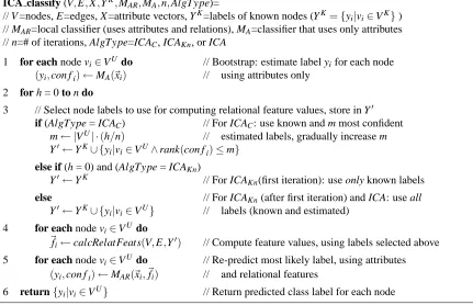
Figure 2 displays pseudocode for ICA, ICAC, and ICAKn, depending on the setting of the parameter
AlgType. We describe each in turn.
5.1.1 ICA
In Figure 2, step 1 is a “bootstrap” step that predicts the class label yi of each node in VU using
only attributes (con fi records the confidence of this prediction, but ICA ignores this information).
The algorithm then iterates (step 2). During each iteration, ICA selects all available labels (step 3), computes the relational features’ values based on these labels (step 4), and then re-predicts the class label of each node using both attributes and relational features (step 5). After iterating, hopefully to convergence, step 6 returns the final set of estimated class labels.
Types of Caution Used: Steps 3-4 of ICA use all available labels for feature computation (including
estimated, possibly incorrect labels) and step 5 picks the single most likely label for each node based on the new predictions. In these steps, uncertainty in the predictions is ignored. Thus, ICA does not
5. Technically, wvRN by itself is a local classifier, not an inference algorithm, but for brevity we refer to the family of algorithms based on this classifier (such as wvRNRL) as wvRN.
6. Section 7 shows that the non-cautious variants ICA, GibbsNC, and LBPNCperform similarly to each other. Thus, our
empirical results would change little if we compared all of the cautious algorithms against the more standard ICA. However, the results for Gibbs and LBP would then concern performance differences between distinct algorithms, due to conjectured but unconfirmed differences in algorithmic properties. By instead comparing Gibbs vs. GibbsNC
and LBP vs. LBPNC, we more precisely demonstrate that the cautious algorithms benefit from specifically identified
Name Cautious Inf.? Key Features Type Evaluated by?
Local classifier-based methods that iteratively classify nodes, yielding a final graph state
ICAC Favors more
conf. labels
Relational features depend only on “more confident” estimated labels; later iterations loosen confidence threshold.
Hard Neville and Jensen (2000); McDowell et al. (2007a)
ICAKn Favors known
labels
First iteration: rel. features depend only on known labels. Later iterations: use all labels.
Hard McDowell et al. (2007a)
ICA Not cautious Always use all labels, known and esti-mated.
Hard Lu and Getoor (2003a); Sen and Getoor (2006); Mc-Dowell et al. (2007a,b)
Local classifier-based algorithms that compute conditional probabilities for each node
Gibbs Samples from
estimated distribution
At each step, classifies using all neigh-bor labels, then samples new la-bels from the resultant distributions. Records new labels to produce final marginal statistics.
Hard Jensen et al. (2004); Neville and Jensen (2007); Sen et al. (2008)
GibbsNC Not cautious Like Gibbs, but always pick most
likely label instead of sampling.
Hard None, but very similar to ICA.
Global formulation algorithms based on loopy belief propagation (LBP)
LBP Reasons with estimated distribution
Passes continuous-valued messages between linked neighbors until con-vergence.
Soft Taskar et al. (2002); Neville and Jensen (2007); Sen et al. (2008)
LBPNC Not cautious Like LBP, but each node always
chooses single most likely label to use for next round of messages.
Hard —
Relational-only algorithms
wvRNRL Reasons with
estimated distribution
Computes new distribution by aver-aging neighbors’ label distributions; combines old and new distributions via relaxation labeling.
Soft Macskassy and Provost (2007); Gallagher et al. (2008)
wvRNICA+C Favors nodes
closer to known labels
Initializes nodes in VU to missing. Computes most likely label by averag-ing neighbors’ labels, ignoraverag-ing
miss-ing labels.
Hard Macskassy and Provost (2007); similar to Galstyan and Cohen (2007)
wvRNICA+NC Not cautious Like wvRNICA+C, but no missing
la-bels are used. Instead, initialize nodes in VUby sampling from the prior label distribution.
Hard —
Table 1: The ten collective inference algorithms considered in this article, divided into four fami-lies. Hard/soft refers to hard-labeling and soft-labeling (see Section 2.2).
perform cautious inference. However, it may exploit cautious learning to learn the classifier models that are used for inference (MAand MAR).
5.1.2 ICAC
In steps 3-4 of Figure 2, ICA assumes that the estimated node labels are all equally likely to be
correct. When AlgType instead selects ICAC, the inference becomes more cautious by only
ICA classify (V,E,X,YK,MAR,MA,n,AlgType)=
// V =nodes, E=edges, X =attribute vectors, YK=labels of known nodes (YK={yi|vi∈VK}) // MAR=local classifier (uses attributes and relations), MA=classifier that uses only attributes // n=# of iterations, AlgType=ICAC, ICAKn, or ICA
1 for each node vi∈VU do // Bootstrap: estimate label yifor each node
(yi,con fi)←MA(~xi) // using attributes only
2 for h = 0 to n do
3 // Select node labels to use for computing relational feature values, store in Y′
if (AlgType = ICAC) // For ICAC: use known and m most confident
m← |VU| ·(h/n) // estimated labels, gradually increase m
Y′←YK∪ {yi|vi∈VU∧rank(con fi)≤m}
else if (h = 0) and (AlgType = ICAKn)
Y′←YK // For ICAKn(first iteration): use only known labels
else // For ICAKn(after first iteration) and ICA: use all
Y′←YK∪ {yi|vi∈VU} // labels (known and estimated)
4 for each node vi∈VU do
~fi←calcRelatFeats(V,E,Y′) // Compute feature values, using labels selected above
5 for each node vi∈VU do // Re-predict most likely label, using attributes
(yi,con fi)←MAR(~xi, ~fi) // and relational features
6 return{yi|vi∈VU} // Return predicted class label for each node
Figure 2: Algorithm for ICA family of algorithms. We use n=10 iterations.
the current estimated labels; other labels are considered missing and thus ignored in the next step. Step 4 computes the relational features using only the committed labels, and step 5 classifies using this information. Step 3 gradually increases the fraction of estimated labels that are committed per iteration (e.g., if n=10, from 0%, 10%, 20%,..., up to 100%). Node label assignments committed in
an iteration h are not necessarily committed again in iteration h+1 (and may in fact change).
ICACrequires some kind of confidence measure (con fiin Figure 2) to determine the “best” m of
the current label assignments (those with the highest confidence “rank”). We adopt the approach of Neville and Jensen (2000) and use the posterior probability of the most likely class for each node i as
con fi. In exploratory experiments, we found that alternative measures (e.g., probability difference of the top two classes) produced similar results.
Types of Caution Used: ICAC favors more confident information by ignoring nodes whose labels
are estimated with lower confidence. Step 3 executes this preference, which affects the algorithm in several ways. First, omitting the estimated labels for some nodes causes the relational feature value computation in step 4 to ignore those less certain labels. Since this computation favors more reliable label assignments, subsequent assignments should also be more reliable. Second, if any node links only to nodes with missing labels, then the computed value of the relational features for that node will also be missing; Section 6.5 describes how the classifier in Step 5 handles this case. Third, recall that a realistic CC scenario’s test set may have links to nodes with known labels; these
nodes, represented by VK, provide the “most certain” labels and thus may aid classification. ICA
C
exploits only these labels for iteration h=0. In this case, step 3 ignores all estimated labels (every
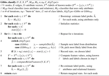
Gibbs classify (V,E,X,YK,MAR,MA,n,nB,C,AlgType)=
// V =nodes, E=edges, X =attribute vectors, YK=labels of known nodes (YK={yi|vi∈VK}) // MAR=local classifier (uses attributes and relations), MA=classifier that uses only attributes // n=# of iterations, nB= “burn-in” iters., C=set of class labels, AlgType=Gibbs or GibbsNC
1 for each node vi∈VU do // Bootstrap: estimate label probs.~bi
~bi←MA(~xi) // for each node, using attributes only
2 for each node vi∈VU do // Initialize statistics
for each c∈C stats[i][c]←0
3 for h = 1 to n do // Repeat for n iterations
for each node vi∈VUdo
4 switch (AlgType):
case (Gibbs): yi←sampleDist(~bi) // Sample next label from distribution case (GibbsNC): yi←argmaxc∈Cbi(c) // Or, pick most likely label from dist. 5 if(h>nB)stats[i,yi]←stats[i,yi] +1 // Record stats. on chosen label 6 Y′←YK∪ {yi|vi∈VU} // Compute feature values, using known
for each node vi∈VUdo // labels and labels chosen in step 4
~fi←computeRelatFeatures(V,E,Y′)
7 for each node vi∈VUdo // Re-estimate label probs., using
~bi←MAR(~xi, ~fi) // attributes and relational features
8 return stats // Return marginal stats. for each node
Figure 3: Algorithm for Gibbs sampling. Thousands of iterations are typically needed.
from VK. Thus, the known labels influence the first classification in step 5, before any estimated
labels are used, and in subsequent iterations. Finally, ICACcan also benefit from PLUL.
5.1.3 ICAKn
The above discussion highlighted two different effects from ICAC: favoring more confident
esti-mated labels vs. favoring known labels from VK. An interesting variant is to favor the known labels
in the first iteration (just like ICAC), but then use all labels for subsequent iterations (just like ICA).
We call this algorithm ICAKn(“ICA+Known”).
Types of Caution Used: ICAKnfavors only known nodes. It is thus more cautious than ICA, but
less cautious than ICAC. It can also benefit from cautious learning via PLUL.
5.2 Gibbs Family of Algorithms
Figure 3 displays pseudocode for Gibbs sampling (Gibbs) and the non-cautious variant GibbsNC.
We describe each in turn.
5.2.1 Gibbs
the most likely class. Step 2 initializes the statistics that will be used to compute the marginal class probabilities for each node. In step 4, within the loop, the algorithm probabilistically samples the current class label distribution of each node and assigns a single label yibased on this distribution.
This label is also recorded in the statistics during Step 5 (after the first nBiterations are ignored for
“burn-in”). Step 6 then selects all labels (known labels and those just sampled) and uses them to compute the relational features’ values. Step 7 re-estimates the posterior class label probabilities given these relational features. The process then repeats. When the process terminates, the statistics recorded in step 5 approximate the marginal distribution of class labels, and are returned by step 8.
Types of Caution Used: Like ICAC, Gibbs is cautious in its use of estimated labels, but in a different
way. In particular, ICACexercises caution in step 3 by ignoring (at least for some iterations) labels
that have lower confidence. In contrast, Gibbs exercises caution by sampling, in step 4, values from each node’s predicted label distribution—causing nodes with lower prediction confidence to reflect that uncertainty via higher fluctuation in their assigned labels, yielding less predictive influence on their neighbors. Gibbs can also benefit from cautious learning via PLUL.
We expect Gibbs to perform better than ICAC, since it makes use of more information, but this
requires careful confirmation. In addition, Gibbs is considerably more time intensive than ICACor
ICA (see Section 5.6).
5.2.2 GibbsNC
GibbsNC is identical to Gibbs except that instead of sampling in step 4, it always selects the most
likely label. This change makes GibbsNCdeterministic (unlike Gibbs), and makes GibbsNCbehave
almost identically to ICA. In particular, observe that after any number of iterations h (1≤h≤n),
ICA and GibbsNC will have precisely the same set of current label assignments for every node.
However, ICA’s result is the final set of label assignments, whereas GibbsNC’s result is the marginal
statistics computed from these time-varying assignments. For a given data set, if ICA converges to
an an unchanging set of label assignments, then for sufficiently large n GibbsNC’s final result (in
terms of accuracy) will be identical to ICA’s. If, however, some nodes’ labels continue to oscillate
with ICA, then ICA and GibbsNCwill have different results for some of those nodes.
Types of Caution Used: Just like ICA, GibbsNC uses all available labels for relational feature
computation, and always picks the single most likely label based on the new predictions. Thus,
GibbsNC does not perform cautious inference, though it can benefit from cautious learning to learn
the classifiers MAand MAR.
5.3 LBP Family of Algorithms
This section describes loopy belief propagation (LBP) and the non-cautious variant LBPNC.
5.3.1 LBP
LBP has been a frequently studied technique for performing approximate inference, and has been
LBP performs inference via passing messages from node to node. In particular, mi→j(c)
repre-sents node vi’s assessment of how likely it is that node vj has a true label of class c. In addition,
φi(c)represents the “non-relational evidence” (e.g., based only on attributes) for vihaving class c,
andψi j(c′,c)represents the “compatibility function” which describes how likely two nodes of class
c and c′ are linked together (in terms of Markov networks, this represents the potential functions defined by the pairwise cliques of linked class nodes). Given these two sets of functions, Yedidia et al. (2000) show the belief that node i has class c can be calculated as follows:
bi(c) =αφi(c)
∏
k∈Nimk→i(c) (1)
whereαis a normalizing factor to ensure that∑c∈Cbi(c) =1 and Ni is the neighborhood function
defined as:
Ni={vj|∃(vi,vj)∈E}.
The messages themselves are computed recursively as:
m′i→j(c) =α
∑
c′∈C
φi(c′)ψi j(c′,c)
∏
k∈Ni\jmk→i(c′) !
. (2)
Observe that the message from i to j incorporates the beliefs of all the neighbors of i (Ni)except j
itself. m′i→j(c)is the “new” value of mi→j(c)to be used in the next iteration.
For CC, we need a model that generalizes from the training nodes to the test nodes. The above equations do not provide this, since they have node-specific potential functions (i.e.,ψi j is specific
to nodes i and j). Fortunately, we can represent each potential function as a log-linear combination of generalizable features, as commonly done for such Markov networks (e.g., Della Pietra et al., 1997; McCallum et al., 2000a). More specifically for CC, Taskar et al. (2002) used a log-linear combination of functions that indicate the presence or absence of particular attributes or other fea-tures. Several papers (e.g., Sen and Getoor, 2006; Sen et al., 2008) have described a general model on how to accomplish this, but do not completely explain how to perform the computation. For a slight loss in generality (e.g., assuming that our nodes are represented by a simple attribute vector),
we now describe how to perform LBP for CC on an undirected graph. In particular, let NA be the
number of attributes,
D
hbe the domain of attribute h, and wc,h,kbe a learned weight indicating howstrongly a value of k for attribute h indicates that a given node has class c. In addition, let fi(h,k)=1
iff the hthattribute of node i is k (i.e., xih=k). Then
φi(c) =exp
∑
h∈{1..NA}∑
k∈Dh
exp(wc,h,k)fi(h,k)) !
which is a special case of logistic regression. We likewise define similar learned weights of the form wc,c′ that indicate how likely a node with label c is linked to a node with label c′, yielding the
compatibility function
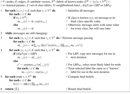
LBP classify (V,E,X,YK,w,C,N,AlgType)=
// V =nodes, E=edges, X =attribute vectors, YK=labels of known nodes (YK={yi|vi∈VK}) // w=learned params., C=set of class labels, N=neighborhood funct., AlgType=LBP or LBPNC
1 for each(vi,vj)∈E such that vj∈VU do // Initialize all messages for each c∈C do
if (vi∈VK) // If class is known (yi), set message to its
mi→j(c)←α·exp(wyi,c) // final, class-specific value
else // Otherwise, message starts with same value
mi→j(c)←α // for every class, but will vary later
2 while (messages are still changing)
3 for each(vi,vj)∈E such that vj∈VUdo // Perform message passing for each c∈C do
m′i→j(c)←α∑c′∈C φi(c′)exp(wc′,c)∏k∈Ni\jmk→i(c ′)
4 for each(vi,vj)∈E such that vj∈VUdo
if (AlgType = LBP) // For LBP, copy new messages for use in
mi→j(c)←m′i→j(c) // next iteration else
c′←argmaxc∈C(m′i→j(c)) // For LBPNC, select most likely label for node
for each c∈C do // Treat selected label the same as a “known”
mi→j(c)←exp(wc′,c) // label for use in the next iteration
5 for each node vi∈VU do // Compute final beliefs
for each c∈C do
bi(c)←αφi(c)∏k∈Nimk→i(c)
6 return{~bi} // Return final beliefs
Figure 4: Algorithm for loopy belief propagation (LBP).αis a normalization factor.
As desired, the compatibility function is now independent of specific node identifiers, that is, it
depends only upon the class labels c and c′, not i and j. We use conjugate gradient descent to learn
the weights (cf., Taskar et al., 2002; Neville and Jensen, 2007; Sen et al., 2008).
Finally, we must consider how to handle messages from nodes with a “known” class label.
Suppose node vi has known class yi. This is equivalent to having a node where the non-relational
evidenceφi(c) =1 if c is yi and zero otherwise. Since yiis known, node vi is not influenced by its
neighbors. In that case, using Equation 2 (with an empty neighborhood for the product) yields:
mi→j(c) =α
∑
c′∈Cφi(c′)ψi j(c′,c) =α·ψi j(yi,c) =α·exp(wyi,c). (3)
Given these formulas, we can now present the complete algorithm in Figure 4. In Step 1, the
messages are initialized, using Equation 3 if vi is a known node; otherwise, each value is set toα
(creating a uniform distribution). Steps 2-4 performs message passing until convergence, based on Equation 2. Finally, step 5 computes the final beliefs using Equation 1 and step 6 returns the results.
Types of Caution Used: Like Gibbs, LBP exercises caution by reasoning based on the estimated
label uncertainty, but in a different manner. Instead of sampling from the estimated distribution,
LBP in step 3 directly updates its beliefs using all of its current beliefs, so that the new beliefs
WVRN RL classify (V,YK,n,C,~bprior,N,Γ)=
// V =nodes, YK=labels of known nodes (YK={yi|vi∈VK}), n=# of iterations // C=set of class labels,~bprior=class priors, N=neighborhood funct.,Γ=decay factor
1 for each node vi∈VKdo // Create belief vector for each known label
~bi←makeBelie f sFromKnownClass(|C|,yi) // (all zeros except at index for class yi)
for each node vi∈VU do // Create initial beliefs for unknown labels
~bi←~bprior // (using class priors as initial setting)
2 for h = 0 to n do // Iteratively re-compute beliefs
3 for each node vi∈VUdo // Compute new distribution for each node
~ b′
i←|N1
i|∑vj∈Ni~bj // by averaging neighbors’ distributions
4 for each node vi∈VUdo // Perform simulated annealing
~bi←Γh~b′
i+ (1−Γh)~bi
5 return{~bi|vi∈VU} // Return belief distribution for each node
Figure 5: Algorithm for wvRNRL. Based on Macskassy and Provost (2007), we use n=100
itera-tions with a decay factor ofΓ=0.99.
by the continuous-valued numbers that represent each message mi→j. LBP can also benefit from
cautious learning with PLUL; in this case, PLUL influences the wc,h,k and wc,c′ weights that are
learned (see Section 6.4).
5.3.2 LBPNC
LBPNC is identical to LBP except that after the new messages are computed in step 3, in step 4
LBPNCpicks the single most likely label c′to represent the message from vito vj. LBPNCthen treats
c′as equivalent to a “known” label yifor viand re-computes the appropriate message mi→j(c)using
Equation 3.
Types of Caution Used: Like ICA and GibbsNC, LBPNCis non-cautious because it uses all available
labels for relational feature computation and always picks the single most likely label based on the new predictions. In essence, the “pick most likely” step transforms the soft-labeling LBP algorithm
into the hard-labeling LBPNC algorithm, removing cautious inference just as the “pick most likely”
step did for GibbsNC. However, LBPNC, like LBP, can still benefit from cautious learning with
PLUL.
5.4 wvRN Family of Algorithms
Figure 5 displays pseudocode for wvRNRL, a soft-labeling algorithm. For simplicity, we present the
related, hard-labeling variants wvRNICA+Cand wvRNICA+NCseparately in Figure 6. Each of these is
a relational-only algorithm; Section 7.9 will discuss variants that incorporate attribute information.
5.4.1 wvRNRL
wvRNRL(Weighted-Vote Relational Neighbor, with relaxation labeling) is a relationonly CC
WVRN ICA classify (V,YK,n,C,~bprior,N,AlgType)=
// V =nodes, YK=labels of known nodes (YK={yi|vi∈VK}), n=# of iters., C=class labels //~bprior=class priors, N=neighborhood function, AlgType=wvRNICA+C or wvRNICA+NC
1 for each node vi∈VU do
switch (AlgType): // Set initial value for unknown labels...
case (wvRNICA+C): yi← ′?′ // ...start labels as missing
case (wvRNICA+NC): yi←sampleDist(~bprior) // ...or sample label from class priors
2 for h = 0 to n do // Iteratively re-label the nodes
3 for each node vi∈VUdo
Ni′← {vj∈Ni|yj6= ′?′} // Find all non-missing neighbors
if(|Ni′|>0) // New label is the most common label
y′i←argmaxc∈C| {vj∈Ni′|yj=c} | // amongst those neighbors
else y′i=yi // If no such neighbors, keep same label
4 for each node vi∈VUdo // After all new labels are computed,
yi←y′i // update to store the new labels
5 return{yi|vi∈VU} // Return est. class label for each node
Figure 6: Algorithm for wvRNICA+Cand wvRNICA+NC. This is a “hard labeling” version of wvRNRL;
each of the 5 steps corresponds to the same numbered step in Figure 5. We use n=100
iterations.
evaluations. At each iteration, each node i updates its estimated class distribution by averaging the
current distributions of each of its linked neighbors. wvRNRL ignores all attributes (non-relational
features). Thus, wvRNRL is useful only if the test set links to some nodes with known labels to
“seed” the inference process. Macskassy and Provost showed that this simple algorithm can work well if the nodes exhibit strong homophily and enough labels are known.
Step 1 of wvRNRL(Figure 5) initializes a belief vector for every node, using the known labels
for nodes in VK, and a class prior distribution for nodes in VU. For each node, step 3 averages the
current distributions of its neighbors, while step 4 performs simulated annealing to ensure conver-gence. Step 5 returns the final beliefs. For simplicity, we omit edge weights from the algorithm’s description, since our experiments do not use them.
Types of Caution Used: Since wvRNRLcomputes directly with the estimated label distributions, it
exercises cautious inference in the same manner as LBP. However, unlike the other CC algorithms, it does not learn from a training set, and thus cautious learning with PLUL does not apply.
5.4.2 wvRNICA+CANDwvRNICA+NC
Figure 6 presents a hard-labeling alternative to wvRNRL. Each of the five steps mirror the
corre-sponding step in the description of wvRNRL. In particular, for node vi, step 3 computes the most
common label among the neighbors of vi (the hard-labeling equivalent of averaging the
distribu-tions), and step 4 commits the new labels without annealing.
that were incorrect but highly self-consistent; leading to errors even when many known labels were
provided. Instead, Macskassy and Provost (2007) suggest initializing each node vi∈VU to missing
(indicated in Figure 6 by a question mark), a value that is ignored during calculations. They call the
resulting algorithm wvRN-ICA; here we refer to it as wvRNICA+C. A missing label remains for node
viafter iteration h if during that iteration every neighbor of viwas also missing.
Alternatively, a simpler algorithm is to always compute with all neighbor labels (do not initialize
any to missing), but initialize each label in VUby sampling from the prior distribution. We call this
algorithm wvRNICA+NC. This process is the hard-labeling analogue of wvRNRL’s approach: instead
of initializing each node with the prior distribution, with wvRNICA+NCsampling initializes the entire
set so that it represents, in aggregate, the prior distribution.
Types of Caution Used: wvRNICA+NCalways uses the estimated label of every node, without regard
for how certain that estimate is. Thus, it does not exhibit cautious inference. However, wvRNICA+C
does exhibit cautious inference, although this effect was not discussed by prior work with this algorithm. In particular, during the first iteration wvRNICA+C uses only the certain labels from YK,
since all nodes in YU are marked missing. These known labels are used to estimate labels for every
node in VU that is directly adjacent to some node in VK. In subsequent iterations, wvRNICA+C
uses both labels from YK and labels from YU that have been estimated so far. However, the labels
estimated so far are likely to be more reliable than later estimations, since the former labels are
from nodes that were closer to at least one known label. Thus, in a manner similar to ICAC’s
gradual commitment of labels based on confidence, wvRNICA+C gradually incorporates more and
more estimated labels into its computation, where more confident labels (those closer to known
nodes) are incorporated sooner. This effect causes wvRNICA+C to exploit estimated labels more
cautiously.
5.5 Parameter Learning for Uncertain Labels (PLUL)
CC algorithms typically train a local classifier on a fully-labeled training set, then use that local classifier with some collective inference algorithm to classify the test set. Unfortunately, this results in asymmetric training and test phases: since all labels are known in the training phase, the learning process sees no uncertainty in relational feature values, unlike the reality of testing. Moreover, the classifier’s training is unaffected by the type of collective inference algorithm used, and how (if at all) that collective algorithm attempts to compensate for the uncertainty of estimated labels during testing. Consequently, the learned classifier may tend to produce poor estimates of important parameters related to the relational features (e.g., feature weights, conditional probabilities). Even for CC algorithms that do not use a local classifier, but instead take a global approach that learns over the entire training graph (as with LBP and relaxation labeling), the same fundamental problem occurs: if autocorrelation is present, then parameters learned over the fully labeled training set tend to overstate the usefulness of relational features for testing, where estimated labels must be used.
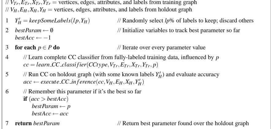
PLUL learn (CCtype,P,l p,VTr,ETr,XTr,YTr,VH,EH,XH,YH)=
// CCtype=CC alg. to use, P=set of parameter values to consider, l p=labeled proportion to use // VTr,ETr,XTr,YTr=vertices, edges, attributes, and labels from training graph
// VH,EH,XH,YH=vertices, edges, attributes, and labels from holdout graph
1 YH′ =keepSomeLabels(l p,YH) // Randomly select lp% of labels to keep; discard others
2 bestParam←/0 // Initialize variables to track best parameter so far
bestAcc← −1
3 for each p∈P do // Iterate over every parameter value
4 // Learn complete CC classifier from fully-labeled training data, influenced by p
cc=learn CC classi f ier(CCtype,VTr,ETr,XTr,YTr,p)
5 // Run CC on holdout graph (with some known labels YH′) and evaluate accuracy
acc←execute CC in f erence(cc,VH,EH,XH,YH′)
6 // Remember this parameter if it’s the best so far
if(acc>bestAcc)
bestParam←p bestAcc←acc
7 return bestParam // Return best parameter found over the holdout graph
Figure 7: Algorithm for Parameter Learning for Uncertain Labels (PLUL). The holdout graph is derived from the original training data and is disjoint from the graph that is used later for testing.
using a k-nearest-neighbor rule as the local classifier, we employ PLUL to adjust the weight wRof
relational features in the node similarity function. PLUL performs automated tuning by repeatedly evaluating different values of the selected parameter, as used by the local classifier, together with the collective inference algorithm (or the entire learned model for LBP). For each parameter value, accuracy is evaluated on a holdout set (a subset of the training set). PLUL then selects the parameter value that yields the best accuracy to use for testing.
Figure 7 summarizes these key steps of PLUL and some additional details. First, note that proper use of PLUL requires a holdout set that reflects the test set conditions. Thus, step 1 of the algorithm removes some or all of the labels from the holdout set, leaving only the same percentage of labels (lp%) that are expected in the test set. Second, running CC inference with a new parameter value may require re-learning the local classifier (for ICA or Gibbs) or the entire learned model (for
LBP). This is shown in step 4 of Figure 7. Alternatively, for Naive Bayes or k-nearest-neighbor
local classifiers, the existing classifier can simply be updated to reflect the new parameter value. We expect PLUL’s utility to vary based upon the fraction of known labels (lp) that are available to the test set. If there are few such labels, there is more discrepancy between the training and test environments, and hence more need to apply PLUL. However, if there are many such labels, then PLUL may not be useful.
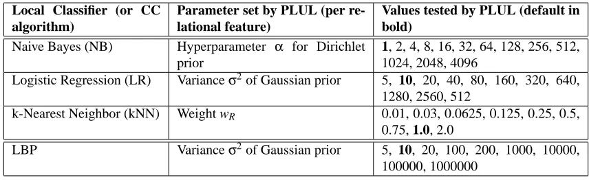
Local Classifier (or CC algorithm)
Parameter set by PLUL (per re-lational feature)
Values tested by PLUL (default in bold)
Naive Bayes (NB) Hyperparameter α for Dirichlet prior
1, 2, 4, 8, 16, 32, 64, 128, 256, 512,
1024, 2048, 4096
Logistic Regression (LR) Varianceσ2of Gaussian prior 5, 10, 20, 40, 80, 160, 320, 640,
1280, 2560, 512
k-Nearest Neighbor (kNN) Weight wR 0.01, 0.03, 0.0625, 0.125, 0.25, 0.5, 0.75, 1.0, 2.0
LBP Varianceσ2of Gaussian prior 5, 10, 20, 100, 200, 1000, 10000,
100000, 1000000
Table 2: The classifiers (NB, LR, and kNN) and CC algorithm (LBP) used in our experiments for which PLUL can be applied to improve performance. The second column lists the key relational parameters that we identified for PLUL to learn, while the last column shows the values that PLUL considers in its cross-validation.
last row demonstrates how it can instead be applied to a global algorithm like LBP. For instance, for the NB classifier, most previous research has used either no prior or a simple Laplacian (“add one”) prior for each conditional probability. By instead using a Dirichlet prior (Heckerman, 1999), we can
adjust the “hyperparameter”αof the prior for each relational feature. Larger values ofαtranslate to
less extreme conditional probabilities, thus tempering the impact of relational features. For the kNN classifier, reducing the weight of relational features has a similar net effect. For the LR classifier and the LBP algorithm, both techniques involve iterative MAP estimation. Increasing the value of the variance of the Gaussian prior for relational features causes the corresponding parameter to “fit” less closely to the training data, again making the algorithm more cautious in its use of such relational features.
While the core mechanism of PLUL—cross-validation tuning—is common, techniques like PLUL to explicitly compensate for the bias incurred from training on a fully-labeled set while testing using estimated labels have not been previously used for CC. A possible exception is Lu and Getoor (2003a), who appear to have used a similar technique to tune a relational parameter, but, in contrast to this work, they did not discuss its need, the specific procedure, or the performance impact.