Hierarchical Average Reward Reinforcement Learning
Mohammad Ghavamzadeh [email protected]
Department of Computing Science University of Alberta
Edmonton, AB T6G 2E8, CANADA
Sridhar Mahadevan [email protected]
Department of Computer Science University of Massachusetts Amherst, MA 01003-4601, USA
Editor: Michael Littman
Abstract
Hierarchical reinforcement learning (HRL) is a general framework for scaling reinforcement learn-ing (RL) to problems with large state and action spaces by uslearn-ing the task (or action) structure to restrict the space of policies. Prior work in HRL including HAMs, options, MAXQ, and PHAMs has been limited to the discrete-time discounted reward semi-Markov decision process (SMDP) model. The average reward optimality criterion has been recognized to be more appropriate for a wide class of continuing tasks than the discounted framework. Although average reward RL has been studied for decades, prior work has been largely limited to flat policy representations.
In this paper, we develop a framework for HRL based on the average reward optimality cri-terion. We investigate two formulations of HRL based on the average reward SMDP model, both for discrete-time and continuous-time. These formulations correspond to two notions of optimality that have been previously explored in HRL: hierarchical optimality and recursive optimality. We present algorithms that learn to find hierarchically and recursively optimal average reward policies under discrete-time and continuous-time average reward SMDP models.
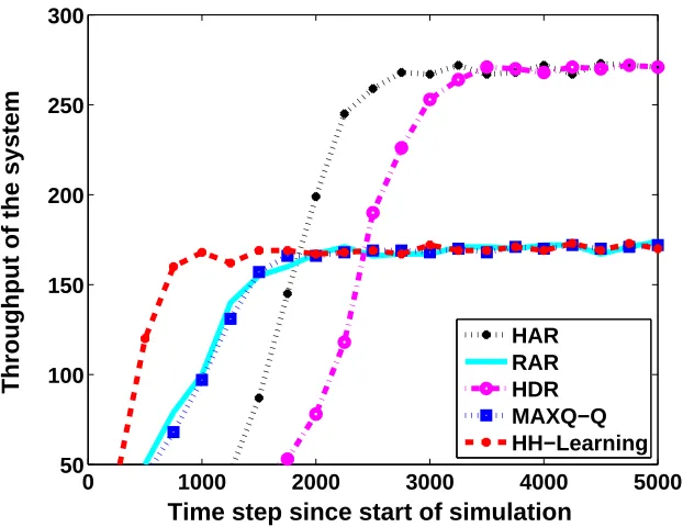
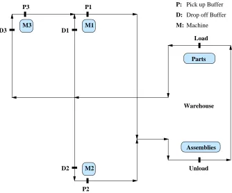
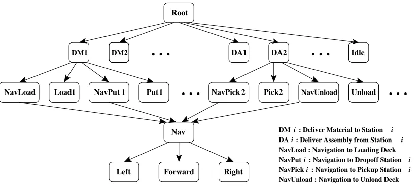
We use two automated guided vehicle (AGV) scheduling tasks as experimental testbeds to study the empirical performance of the proposed algorithms. The first problem is a relatively simple AGV scheduling task, in which the hierarchically and recursively optimal policies are different. We compare the proposed algorithms with three other HRL methods, including a hierarchically optimal discounted reward algorithm and a recursively optimal discounted reward algorithm on this problem. The second problem is a larger AGV scheduling task. We model this problem using both discrete-time and continuous-time models. We use a hierarchical task decomposition in which the hierarchically and recursively optimal policies are the same for this problem. We compare the performance of the proposed algorithms with a hierarchically optimal discounted reward algorithm and a recursively optimal discounted reward algorithm, as well as a non-hierarchical average reward algorithm. The results show that the proposed hierarchical average reward algorithms converge to the same performance as their discounted reward counterparts.
1. Introduction
Sequential decision making under uncertainty is a fundamental problem in artificial intelligence (AI). Many sequential decision making problems can be modeled using the Markov decision process (MDP) formalism. A MDP (Howard, 1960; Puterman, 1994) models a system that we are interested in controlling as being in some state at each time step. As a result of actions, the system moves through some sequence of states and receives a sequence of rewards. The goal is to select actions to maximize (minimize) some measure of long-term reward (cost), such as the expected discounted sum of rewards (costs), or the expected average reward (cost).
Reinforcement learning (RL) is a machine learning framework for solving sequential decision-making problems. Despite its successes in a number of different domains, including backgammon (Tesauro, 1994), job-shop scheduling (Zhang and Dietterich, 1995), dynamic channel allocation (Singh and Bertsekas, 1996), elevator scheduling (Crites and Barto, 1998), and helicopter flight control (Ng et al., 2004), current RL methods do not scale well to high dimensional domains—they can be slow to converge and require many training samples to be practical for many real-world problems. This issue is known as the curse of dimensionality: the exponential growth of the number of parameters to be learned with the size of any compact encoding of system state (Bellman, 1957). Recent attempts to combat the curse of dimensionality have turned to principled ways of exploiting abstraction in RL. This leads naturally to hierarchical control architectures and associated learning algorithms.
Hierarchical reinforcement learning (HRL) is a general framework for scaling RL to problems with large state spaces by using the task (or action) structure to restrict the space of policies. Hi-erarchical decision making represents policies over fully or partially specified temporally extended actions. Policies over temporally extended actions cannot be simply treated as single-step actions over a coarser time scale, and therefore cannot be represented in the MDP framework since actions take variable durations of time. Semi-Markov decision process (SMDP) (Howard, 1971; Puterman, 1994) is a well-known statistical framework for modeling temporally extended actions. Action du-ration in a SMDP can depend on the transition that is made. The state of the system may change continually between actions, unlike MDPs where state changes are only due to actions. Therefore, SMDPs have become the main mathematical model underlying HRL methods.
In this paper, we extend previous work on HRL to the average reward setting, and investigate two formulations of HRL based on average reward SMDPs. These two formulations correspond to two notions of optimality in HRL: hierarchical optimality and recursive optimality (Dietterich, 2000). We extend the MAXQ hierarchical RL method (Dietterich, 2000) and introduce a HRL framework for simultaneous learning of policies at multiple levels of a task hierarchy. We then use this HRL framework to derive discrete-time and continuous-time algorithms that learn to find hier-archically and recursively optimal average reward policies. In these algorithms, we assume that the overall task (the root of the hierarchy) is continuing. Hierarchically optimal average reward RL (HAR) algorithms find a hierarchical policy within the space of policies defined by the hierarchical decomposition that maximizes the global gain. Recursively optimal average reward RL (RAR) algorithms treat non-primitive subtasks as continuing average reward problems, where the goal at each subtask is to maximize its gain given the policies of its children. We investigate the conditions under which the policy learned by RAR algorithm at each subtask is independent of the context in which it is executed and therefore can be reused by other hierarchies. We use two automated guided vehicle (AGV) scheduling tasks as experimental testbeds to study the empirical performance of the proposed algorithms. The first problem is a relatively simple AGV scheduling task, in which the hierarchically and recursively optimal policies are different. We compare the proposed algorithms with three other HRL methods, including a hierarchically optimal discounted reward algorithm and a recursively optimal discounted reward algorithm on this problem. The second problem is a relatively larger AGV scheduling task. We model this problem using both discrete-time and continuous-time models. We use a hierarchical task decomposition where the hierarchically and recursively optimal policies are the same. We compare the performance of the proposed algorithms with a hierarchi-cally optimal discounted reward algorithm and a recursively optimal discounted reward algorithm, as well as a non-hierarchical average reward algorithm. The results show that the proposed hier-archical average reward algorithms converge to the same performance as their discounted reward counterparts.
The rest of this paper is organized as follows. Section 2 provides a brief overview of HRL. In Section 3, we concisely describe discrete-time SMDPs, and discuss average reward optimality in this model. Section 4 describes the HRL framework, which is used to develop the algorithms of this paper. In Section 5, we extend the previous work on HRL to the average reward setting, and study two formulations of HRL based on the average reward SMDP model. In Section 5.1, we present discrete-time and continuous-time hierarchically optimal average reward RL (HAR) algorithms. In Section 5.2, we investigate different methods to formulate subtasks in a recursively optimal hierar-chical average reward RL setting, and present discrete-time and continuous-time recursively optimal average reward RL (RAR) algorithms. We demonstrate the type of optimality achieved by HAR and RAR algorithms as well as their empirical performance and convergence speed compared to other algorithms using two AGV scheduling problems in Section 6. Section 7 summarizes the paper and discusses some directions for future work. For convenience, a table of the symbols used in this paper is given in Appendix A.
2. An Overview of Hierarchical Reinforcement Learning
policies for simpler subtasks. Subtasks form the basis of hierarchical specifications of action se-quences because they can include other subtasks in their definitions. It is similar to the familiar idea of subroutines from programming languages. A subroutine can call other subroutines as well as execute primitive commands. A subtask as an open-loop control policy is inappropriate for most interesting control purposes, especially the control of stochastic systems. HRL methods generalize the subtask idea to closed-loop policies or, more precisely, closed-loop partial policies because they are generally defined for a subset of the state space. The partial policies must also have well-defined termination conditions. The partial policies with well-defined termination conditions are sometimes called temporally extended actions. Work in HRL has followed three trends: focusing on subsets of the state space in a divide and conquer approach (state space decomposition), grouping sequences or sets of actions together (temporal abstraction), and ignoring differences between states based on the context (state abstraction). Much of the work in HRL falls into several of these categories. Barto and Mahadevan (2003) provide a more detailed introduction to HRL.
Mahadevan and Connell (1992) were among the first to systematically investigate the use of task structure to accelerate RL. In their work, the robot was given a pre-specified task decomposition, and learned a set of local policies instead of an entire global policy. Singh (1992) investigated reinforcement learning using abstract actions of different temporal granularity using a hierarchy of models with variable temporal resolution. Singh applied the mixture of experts framework as a special-purpose task selection architecture to switch between abstract actions. Kaelbling (1993a,b) investigated using subgoals to learn sub-policies. Dayan and Hinton (1993) describe Feudal RL, a hierarchical technique which uses both temporal abstraction and state abstraction to recursively partition the state space and the time scale from one level to the next.
One key limitation of all the above methods is that decisions in HRL are no longer made at synchronous time steps, as is traditionally assumed in RL. Instead, agents make decisions intermit-tently, where each epoch can be of variable length, such as when a distinguishing state is reached (e.g., an intersection in a robot navigation task), or a subtask is completed (e.g., the elevator arrives on the first floor). Fortunately, a well-known statistical model is available to treat variable length actions: the semi-Markov decision process (SMDP) model (Howard, 1971; Puterman, 1994). In a SMDP, state-transition dynamics is specified not only by the state where an action was taken, but also by parameters specifying the length of time since the action was taken. Early work on the SMDP model extended algorithms such as Q-learning to continuous-time (Bradtke and Duff, 1995; Mahadevan et al., 1997b). The early work on SMDP was then expanded to include hierarchical task models over fully or partially specified lower level subtasks, which led to developing powerful HRL models such as hierarchies of abstract machines (HAMs) (Parr, 1998), options (Sutton et al., 1999; Precup, 2000), MAXQ (Dietterich, 2000), and programmable HAMs (PHAMs) (Andre and Russell, 2001; Andre, 2003).
and thus represents the value of a state within that SMDP as composed of the reward for taking an action at that state (which might be composed of many rewards along a trajectory through a subtask) and the expected reward for completing the subtask. To isolate the subtask from the calling context, MAXQ uses the notion of a pseudo-reward. At the terminal states of a subtask, the agent is rewarded according to the pseudo-reward, which is set a priori by the designer, and does not depend on what happens after leaving the current subtask. Each subtask can then be treated in isolation from the rest of the problem with the caveat that the solutions learned are only recursively optimal. Each action in the recursively optimal policy is optimal with respect to the subtask containing the action, all descendant subtasks, and the pseudo-reward chosen by the designer of the system. Another important contribution of MAXQ is the idea that state abstraction can be done separately on the different components of the value function, which allows one to perform dynamic abstraction. We describe the MAXQ framework and related concepts such as recursive optimality and value function decomposition in Section 4. In the PHAM model, Andre and Russell extended HAMs and presented an agent-design language for RL. Andre and Russell (2002) also addressed the issue of safe state abstraction in their model. Their method yields state abstraction while maintaining hierarchical optimality.
3. Discrete-time Semi-Markov Decision Processes
Semi-Markov decision processes (SMDPs) (Howard, 1971; Puterman, 1994) extend the Markov decision process (MDP) (Howard, 1971; Puterman, 1994) model by allowing actions that can take multiple time steps to complete. Note that SMDPs do not theoretically provide additional expres-sive power but they do provide a convenient formalism for temporal abstraction. The duration of an action can depend on the transition that is made.1 The state of the system may change contin-ually between actions unlike MDPs where state changes are only due to actions. Thus, SMDPs have become the preferred language for modeling temporally extended actions (Mahadevan et al., 1997a) and, as a result, the main mathematical model underlying hierarchical reinforcement learn-ing (HRL).
A SMDP is defined as a five tuple h
S
,A
,P
,R
,I
i. All components are defined as in a MDP except the transition probability functionP
and the reward functionR
.S
is the set of states of the world,A
is the set of possible actions from which the agent may choose on at each decision epoch, andI
:S
→ [0,1] is the initial state distribution. The transition probability functionP
now takes the duration of the actions into account. The transition probability functionP
:S
×N×
S
×A
→[0,1]is a multi-step transition probability function (Nis the set of natural numbers), where P(s0,N|s,a) denotes the probability that action a will cause the system to transition from state s to state s0 in N time steps. This transition is at decision epochs only. Basically, the SMDP model represents snapshots of the system at decision points, whereas the so-called natural process describes the evolution of the system over all times. If we marginalize P(s0,N|s,a)over N, we will obtain F(s0|s,a) the transition probability for the embedded MDP. The term F(s0|s,a)denotes the probability that the system occupies state s0at the next decision epoch, given that the decision maker chooses action a in state s at the current decision epoch. The key difference in the reward function for SMDPs is that the rewards can accumulate over the entire duration of an action. As a result, the reward in a SMDP for taking an action in a state depends on the evolution of the system during the execution of the action. Formally, the reward in a SMDP is modeled as a functionR
:S
×A
→R(Ris the set of real numbers), with r(s,a)representing the expected total reward between two decision epochs, given that the system occupies state s at the first decision epoch and the agent chooses action a. This expected reward contains all necessary information about the reward to analyze the SMDP model. For each transition in a SMDP, the expected number of time steps until the next decision epoch is defined as
y(s,a) =E[N|s,a] =
∑
N∈NN
∑
s0∈S
P(s0,N|s,a).
The notion of policy and the various forms of optimality are the same for SMDPs as for MDPs. In infinite-horizon SMDPs, the goal is to find a policy that maximizes either the expected discounted reward or the average expected reward. We discuss the average reward optimality criterion for the SMDP model in the next section.
3.1 Average Reward Semi-Markov Decision Processes
The theory of infinite-horizon SMDPs with the average reward optimality criterion is more complex than that for discounted models (Howard, 1971; Puterman, 1994). The aim of average reward SMDP algorithms is to compute policies that yield the highest average reward or gain. The average reward or gain of a policy µ at state s, gµ(s), can be defined as the ratio of the expected total reward and the expected total number of time steps of following policy µ starting at state s
gµ(s) =lim inf
n→∞
E∑n−t=01r(st,µ(st))|s0=s,µ
E∑n−t=01Nt|s0=s,µ
.
In this equation, Ntis the total number of time steps until the next decision epoch, when agent takes
action µ(st)in state st.
A key observation that greatly simplifies the design of average reward algorithms is that for unichain SMDPs,2the gain of any policy is state independent, that is
gµ(s) =gµ=lim inf
n→∞
E∑n−t=01r(st,µ(st))|µ
E∑n−t=01Nt|µ
, ∀s∈
S
. (1)To simplify exposition, we consider only unichain SMDPs in this paper. When the state space of a SMDP,
S
, is finite or countable, Equation 1 can be written asgµ=F¯
µ
rµ ¯
Fµyµ, (2)
where Fµand ¯Fµ=limn→∞1n∑n−t=01(Fµ)t are the transition probability matrix and the limiting matrix
of the embedded Markov chain for policy µ, respectively,3and rµand yµare vectors with elements r(s,µ(s))and y(s,µ(s)), for all s∈
S
. Under the unichain assumption, ¯F has equal rows, andthere-fore the right hand side of Equation 2 is a vector with elements all equal to gµ.
2. In unichain SMDPs, the underlying Markov chain for every stationary policy has a single recurrent class, and a (possibly empty) set of transient states.
In the average reward SMDP model, a policy µ is measured using a different value function, namely the average-adjusted sum of rewards earned following that policy4
Hµ(s) = lim
n→∞E (
n−1
∑
t=0
[r(st,µ(st))−gµy(st,µ(st))]|s0=s,µ
)
.
The term Hµ is usually referred to as the average-adjusted value function. Furthermore, the average-adjusted value function satisfies the Bellman equation
Hµ(s) =r(s,µ(s))−gµy(s,µ(s)) +
∑
s0∈S,N∈NP(s0,N|s,µ(s))Hµ(s0).
Similarly, the average-adjusted action-value function for a policy µ, Lµ, is defined, and it satisfies the Bellman equation
Lµ(s,a) =r(s,a)−gµy(s,a) +
∑
s0∈S,N∈NP(s0,N|s,a)Lµ(s0,µ(s0)).
4. A Framework for Hierarchical Reinforcement Learning
In this section, we describe a general hierarchical reinforcement learning (HRL) framework for si-multaneous learning of policies at multiple levels of a hierarchy. Our treatment builds upon existing methods, including HAMs (Parr, 1998), options (Sutton et al., 1999; Precup, 2000), MAXQ (Di-etterich, 2000), and PHAMs (Andre and Russell, 2002; Andre, 2003), and, in particular, uses the MAXQ value function decomposition. We extend the MAXQ framework by including the three-part value function decomposition (Andre and Russell, 2002) to guarantee hierarchical optimality, as well as reward shaping (Ng et al., 1999) to reduce the burden of exploration. Rather than redun-dantly explain MAXQ and then our hierarchical framework, we will present our model and note throughout this section where the key pieces were inspired by or are directly related to MAXQ. In the next section, we will extend this framework to the average reward model and present our hierarchical average reward reinforcement learning algorithms.
4.1 Motivating Example
In the HRL framework, the designer of the system imposes a hierarchy on the problem to incorporate domain knowledge and thereby reduces the size of the space that must be searched to find a good policy. The designer recursively decomposes the overall task into a collection of subtasks that are important for solving the problem.
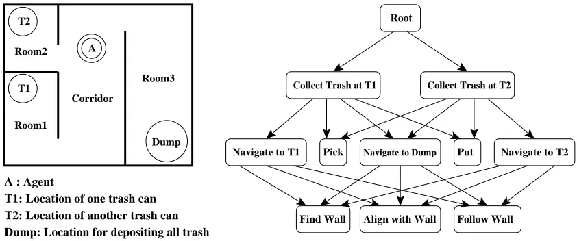
Let us illustrate the main ideas using a simple search task shown in Figure 1. Consider the do-main of an office-type environment (with rooms and connecting corridors), where a robot is assigned the task of picking up trash from trash cans (T 1 and T 2) over an extended area and accumulating it into one centralized trash bin (Dump). For simplicity, we assume that the robot can observe its true location in the environment. The main subtasks in this problem are root (the whole trash-collection task), collect trash at T 1 and T 2, navigate to T 1, T 2, and Dump. Each of these subtasks is defined by a set of termination states. After defining subtasks, we must indicate, for each subtask, which
4. This limit assumes that all policies are aperiodic. For periodic policies, it changes to the Cesaro limit Hµ(s) =
limn→∞1n∑ n−1
k=0E
∑k
other subtasks or primitive actions it should employ to reach its goal. For example, navigate to T 1, T 2, and Dump use three primitive actions find wall, align with wall, and follow wall. Collect trash at T 1 uses two subtasks, navigate to T 1 and Dump, plus two primitive actions Put and Pick, and so on. Similar to MAXQ, all of this information can be summarized by a directed acyclic graph called task graph. The task graph for the trash-collection problem is shown in Figure 1. This hi-erarchical model is able to support state abstraction (while the agent is moving toward the Dump, the status of trash cans T 1 and T 2 is irrelevant and cannot affect this navigation process. Therefore, the variables defining the status of trash cans T 1 and T 2 can be removed from the state space of the navigate to Dump subtask), and subtask sharing (if the system could learn how to solve the navigate to Dump subtask once, then the solution could be shared by both collect trash at T 1 and T 2 subtasks.)
Collect Trash at T1 Collect Trash at T2
Navigate to T1 Pick Navigate to Dump Put Navigate to T2 Root
Find Wall Align with Wall Follow Wall Room3
Corridor A
Dump T2
T1
Room1 Room2
A : Agent
Dump: Location for depositing all trash T2: Location of another trash can T1: Location of one trash can
Figure 1: A robot trash-collection task and its associated task graph.
Like HAMs (Parr, 1998), options (Sutton et al., 1999; Precup, 2000), MAXQ (Dietterich, 2000), and PHAMs (Andre and Russell, 2001; Andre, 2003), this framework also relies on the theory of SMDPs. While SMDP theory provides the theoretical underpinnings of temporal abstraction by modeling actions that take varying amounts of time, the SMDP model provides little in the way of concrete representational guidance, which is critical from a computational point of view. In particular, the SMDP model does not specify how tasks can be broken up into subtasks, how to decompose value functions etc. We examine these issues next.
As in MAXQ, a task hierarchy such as the one illustrated above can be modeled by decompos-ing the overall task MDP
M
, into a finite set of subtasks{M0,M1, . . . ,Mm−1},5where M0is the root task. Solving M0solves the entire MDPM
.Definition 1: Each non-primitive subtask Mi(Mi is not a primitive action) consists of five
compo-nentshSi,Ii,Ti,Ai,Rii:
• Siis the state space for subtask Mi. It is described by those state variables that are relevant to
subtask Mi. The range of a state variable describing Simight be a subset of its range in
S
(thestate space of MDP
M
).• Ii⊆Siis the initiation set for subtask Mi. Subtask Mican be initiated only in states belonging
to Ii.
• Ti⊆Si is the set of terminal states for subtask Mi. Subtask Mi terminates when it reaches
a state in Ti. A policy for subtask Mi can only be executed if the current state s belongs to
(Si−Ti).
• Ai is the set of actions that can be performed to achieve subtask Mi. These actions can be
either primitive actions from
A
(the set of primitive actions for MDPM
), or they can be other subtasks. Technically, Aiis a function of states, since it may differ from one state to another.However, we will suppress this dependence in our notation.
• Riis the reward structure inside subtask Miand could be different from the reward function
of MDP
M
. Here, we use the idea of reward shaping (Ng et al., 1999) and define a more general reward structure than MAXQ’s. Reward shaping is a method for guiding an agent toward a solution without constraining the search space. Besides the reward of the overall task MDPM
, each subtask Mican use additional rewards to guide its local learning.Addi-tional rewards are only used inside each subtask and do not propagate to upper levels in the hierarchy. If the reward structure inside a subtask is different from the reward function of the overall task, we need to define two types of value functions for each subtask, internal value function and external value function. Internal value function is defined based on both the local reward structure of the subtask and the reward of the overall task, and only is used in learning the subtask. On the other hand, external value function is defined only based on the reward function of the overall task and is propagated to the higher levels in the hierarchy to be used in learning the global policy. This reward structure for each subtask in our framework is more general than the one in MAXQ, and of course, includes MAXQ’s pseudo-reward.6
Each primitive action a is a primitive subtask in this decomposition, such that a is always executable and it terminates immediately after execution. From now on in this paper, we use subtask to refer to non-primitive subtasks.
4.2 Policy Execution
If we have a policy for each subtask in a hierarchy, we can define a hierarchical policy for the model.
Definition 2: A hierarchical policy µ is a set of policies, one policy for each subtask in the
hierar-chy: µ={µ0, . . . ,µm−1}.
The hierarchical policy is executed using a stack discipline, similar to ordinary programming languages. Each subtask policy takes a state and returns the name of a primitive action to execute or the name of a subtask to invoke. When a subtask is invoked, its name is pushed onto the Task-Stack and its policy is executed until it enters one of its terminal states. When a subtask terminates, its name is popped off the Task-Stack. If any subtask on the Task-Stack terminates, then all subtasks below it are immediately aborted, and control returns to the subtask that had invoked the terminated subtask. Hence, at any time, the root task is located at the bottom and the subtask which is currently being executed is located at the top of the Task-Stack.
Under a hierarchical policy µ, we define a multi-step transition probability Piµ: Si×N×Si →
[0,1]for each subtask Miin the hierarchy, where Piµ(s0,N|s)denotes the probability that hierarchical
policy µ will cause the system to transition from state s to state s0in N primitive steps at subtask Mi.
We also define a multi-step abstract transition probability Fiµ: Si×N×Si→[0,1]for each subtask
Mi under the hierarchical policy µ. The term Fiµ(s0,N|s) denotes the N-step abstract transition
probability from state s to state s0 under hierarchical policy µ at subtask Mi, where N is the number
of actions taken by subtask Mi, not the number of primitive actions taken in this transition. In this
paper, we use the multi-step abstract transition probability Fiµto model state transition at the subtask level, and the multi-step transition probability Piµ to model state transition at the level of primitive actions. For N=1, Fiµ(s0,1|s)is the transition probability for the embedded MDP at subtask Mi.
We can write Fiµ(s0,1|s)as Fiµ(s0|s), and it can also be obtained by marginalizing Piµ(s0,N|s)over N as described in Section 3.
4.3 Local versus Global Optimality
Using a hierarchy reduces the size of the space that must be searched to find a good policy. However, a hierarchy constrains the space of possible policies so that it may not be possible to represent the optimal policy or its value function, and hence make it impossible to learn the optimal policy. If we cannot learn the optimal policy, the next best target would be to learn the best policy that is consis-tent with the given hierarchy. Two notions of optimality have been explored in the previous work on hierarchical reinforcement learning, hierarchical optimality and recursive optimality (Dietterich, 2000).
Definition 3: A hierarchically optimal policy for MDP
M
is a hierarchical policy which has the best performance among all policies consistent with the given hierarchy. In other words, hierarchi-cal optimality is a global optimum consistent with the given hierarchy. In this form of optimality, the policy for each individual subtask is not necessarily locally optimal, but the policy for the entire hierarchy is optimal. The HAMQ HRL algorithm (Parr, 1998) and the SMDP Q-learning algorithm for a fixed set of options (Sutton et al., 1999; Precup, 2000) both converge to a hierarchicallyopti-mal policy.
con-verges to a recursively optimal policy.
4.4 Value Function Definitions
For recursive optimality, the goal is to find a hierarchical policy µ={µ0, . . . ,µm−1} such that for each subtask Mi in the hierarchy, the expected cumulative reward of executing policy µi and the
policies of all descendants of Mi is maximized. In this case, the value function to be learned for
subtask Mi under hierarchical policy µ must contain only the reward received during the execution
of subtask Mi. We call this the projected value function after Dietterich (2000), and define it as
follows:
Definition 5: The projected value function of a hierarchical policy µ on subtask Mi, denoted ˆVµ(i,s),
is the expected cumulative reward of executing policy µi and the policies of all descendants of Mi
starting in state s∈Siuntil Miterminates.
The expected cumulative reward outside a subtask is not a part of its projected value function. It makes the projected value function of a subtask dependent only on the subtask and its descendants. On the other hand, for hierarchical optimality, the goal is to find a hierarchical policy that max-imizes the expected cumulative reward. In this case, the value function to be learned for subtask Miunder hierarchical policy µ must contain the reward received during the execution of subtask Mi,
and the reward after subtask Miterminates. We call this the hierarchical value function, following
Dietterich (2000). The hierarchical value function of a subtask includes the expected reward outside the subtask and therefore depends on the subtask and all its ancestors up to the root of the hierar-chy. In the case of hierarchical optimality, we need to consider the contents of the Task-Stack as an additional part of the state space of the problem, since a subtask might be shared by multiple parents.
Definition 6:Ωis the space of possible values of the Task-Stack for hierarchy
H
.Let us define joint state space
X
=Ω×S
for the hierarchyH
as the cross product of the set of the Task-Stack values Ω and the state spaceS
. We also define a transition probability func-tion of the Markov chain that results from flattening the hierarchy using the hierarchical policy µ, mµ:X
×X
→[0,1], where mµ(x0|x)denotes the probability that the hierarchical policy µ will causethe system to transition from state x= (ω,s)to state x0= (ω0,s0) at the level of primitive actions. We will use this transition probability function in Section 5.1 to define global gain for a hierarchi-cal policy. Finally, we define the hierarchihierarchi-cal value function using the joint state space
X
as follows:Definition 7: A hierarchical value function for subtask Mi in state x= (ω,s) under hierarchical
policy µ, denoted Vµ(i,x), is the expected cumulative reward of following the hierarchical policy µ
starting in state s∈Siand Task-Stackω.
The current subtask Miis a part of the Task-Stackωand as a result is a part of the state x. So we
can exclude it from the hierarchical value function notation and write Vµ(i,x) as Vµ(x). However
Theorem 1: Under a hierarchical policy µ, each subtask Mican be modeled by a SMDP consisting
of components(Si,Ai,Piµ,R¯i), where ¯Ri(s,a) =Vˆµ(a,s)for all a∈
A
i.This theorem is similar to Theorem 1 in Dietterich (2000). Using this theorem, we can define a recursive optimal policy for MDP
M
with hierarchical decomposition{M0,M1, . . . ,Mm−1}as a hierarchical policy µ={µ0, . . . ,µm−1}such that for each subtask Mi, the corresponding policy µiisoptimal for the SMDP defined by the tuple(Si,Ai,Piµ,R¯i).
4.5 Value Function Decomposition
A value function decomposition splits the value of a state or a state-action pair into multiple ad-ditive components. Modularity in the hierarchical structure of a task allows us to carry out this decomposition along subtask boundaries. In this section, we first describe the two-part or MAXQ decomposition proposed by Dietterich (2000), and then the three-part decomposition proposed by Andre and Russell (2002). We use both decompositions in our hierarchical average reward frame-work depending on the type of optimality (hierarchical or recursive) that we are interested in.
The two-part value function decomposition is at the center of the MAXQ method. The purpose of this decomposition is to decompose the projected value function of the root task, ˆVµ(0,s), in terms of the projected value functions of all the subtasks in the hierarchy. The projected value of subtask Miat state s under hierarchical policy µ can be written as
ˆ
Vµ(i,s) =E
" ∞
∑
k=0 γkr(s
k,ak)|s0=s,µ
#
. (3)
Now, let us suppose that the first action chosen by µi is invoked and executed for a number of
primitive steps N and terminates in state s0according to Piµ(s0,N|s). We can rewrite Equation 3 as
ˆ
Vµ(i,s) =E
" N−1
∑
k=0 γkr(s
k,ak) +
∞
∑
k=N
γkr(s
k,ak)|s0=s,µ
#
. (4)
The first summation on the right-hand side of Equation 4 is the discounted sum of rewards for executing subtask µi(s) starting in state s until it terminates. In other words, it is ˆVµ(µi(s),s), the
projected value function of the child task µi(s). The second term on the right-hand side of the
equation is the projected value of state s0 for the current task Mi, ˆVµ(i,s0), discounted byγN, where
s0 is the current state when subroutine µi(s)terminates and N is the number of transition steps from
state s to state s0. We can therefore write Equation 4 in the form of a Bellman equation:
ˆ
Vµ(i,s) =Vˆµ(µi(s),s) +
∑
N,s0∈Si
Piµ(s0,N|s)γNVˆµ(i
,s0). (5)
Equation 5 can be restated for the projected action-value function as follows:
ˆ
Qµ(i,s,a) =Vˆµ(a,s) +
∑
N,s0∈Si
Piµ(s0,N|s,a)γNQˆµ(i,s0,µi(s0)).
The right-most term in this equation is the expected discounted cumulative reward of completing subtask Mi after executing action a in state s. Dietterich called this term completion function and
denoted it by
Cµ(i,s,a) =
∑
N,s0∈Si
With this definition, we can express the projected action-value function recursively as
ˆ
Qµ(i,s,a) =Vˆµ(a,s) +Cµ(i,s,a), (7)
and we can rewrite the definition for projected value function as
ˆ
Vµ(i,s) =
ˆ
Qµ(i,s,µi(s)) if Miis a non-primitive subtask,
r(s,i) if Miis a primitive action.
(8)
Equations 6 to 8 are referred to as two-part value function decomposition equations for a hi-erarchy under a hierarchical policy µ. These equations recursively decompose the projected value function for the root into the projected value functions for the individual subtasks, M1, . . . ,Mm−1, and the individual completion functions Cµ(j,s,a),j=1, . . . ,m−1. The fundamental quantities that
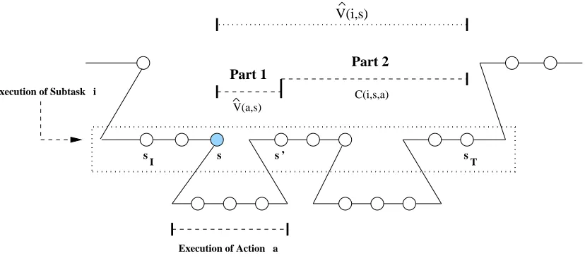
must be stored to represent this value function decomposition are the C values for all non-primitive subtasks and the V values for all primitive actions.7 The two-part value function decomposition is summarized graphically in Figure 2. As mentioned in Section 4.4, since the expected reward after execution of subtask Mi is not a component of the projected action-value function, the two-part
value function decomposition allows only for recursive optimality.
V(i,s)
V(a,s)
Part 1 Part 2
C(i,s,a)
s ’
Execution of Subtask i
s s
I s T
Execution of Action a
Figure 2: This figure shows the two-part decomposition for ˆV(i,s), the projected value function of subtask Mi for the shaded state s. Each circle is a state of the SMDP visited by the agent.
Subtask Mi is initiated at state sI and terminates at state sT. The projected value function
ˆ
V(i,s)is broken into two parts: Part 1) the projected value function of subtask Ma for
state s, and Part 2) the completion function, the expected discounted cumulative reward of completing subtask Miafter executing action a in state s.
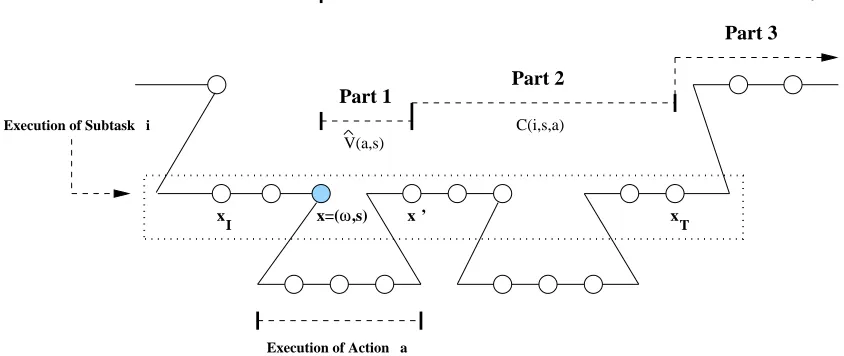
Andre and Russell (2002) proposed a three-part value function decomposition to achieve hi-erarchical optimality. They added a third component for the expected sum of rewards outside the current subtask to the two-part value function decomposition. This decomposition decomposes the hierarchical value function of each subtask into three parts. As shown in Figure 3, these three parts
correspond to executing the current action (which might itself be a subtask), completing the rest of the current subtask (so far is similar to the MAXQ decomposition), and all actions outside the current subtask.
x=( ,s)ω
V(a,s)
Part 1 Part 2
C(i,s,a)
Part 3
Execution of Subtask i
I xT
x x ’
V(i,x)
Execution of Action a
Figure 3: This figure shows the three-part decomposition for V(i,x), the hierarchical value function of subtask Mifor the shaded state x= (ω,s). Each circle is a state of the SMDP visited by
the agent. Subtask Mi is initiated at state xI and terminates at state xT. The hierarchical
value function V(i,x)is broken into three parts: Part 1) the projected value function of subtask Mafor state s, Part 2) the completion function, the expected discounted
cumula-tive reward of completing subtask Mi after executing action a in state s, and Part 3) the
sum of all rewards after termination of subtask Mi.
5. Hierarchical Average Reward Reinforcement Learning
As described in Section 1, the average reward formulation is more appropriate for a wide class of continuing tasks including manufacturing, scheduling, queuing, and inventory control than the more well-studied discounted framework. Moreover, average reward optimality allows for more efficient state abstraction in HRL than the discounted reward formulation. Consider the case that a set of state variables
Y
a is irrelevant for the result distribution of action (subtask) Ma, when Maisexecuted under subtask Mi. It means that for all policies executed by Ma and its descendants, and
for all pairs of states s1and s2in Si(the state space of subtask Mi) that differ only in their values for
the state variables in
Y
a, we havePiµ(s0,N|s1,a) =Piµ(s0,N|s2,a) , ∀s0∈Si , ∀N∈N.
Dietterich (2000) first defined this condition and called it result distribution irrelevance. If this condition is satisfied for subtask Ma, then the completion function values of its parent task Mi
can be represented compactly, that is, all states s∈Si that differ only in their values for the state
variables in
Y
ahave the same completion function, and therefore their completion function valuesThe definition of result distribution irrelevance can be weakened to eliminate N, the number of steps. All that is needed is that for all pairs of states s1and s2in Sithat differ only in the irrelevant
state variables, Fiµ(s0|s1,a) =Fiµ(s0|s2,a)for all s0∈Si. Although the result distribution irrelevance
condition would rarely be satisfied, we often find cases where the weakened result distribution irrelevance condition is true.
Under this revised definition, the compact representation of a completion function still holds in the undiscounted case, but not in the discounted formulation. Consider, for example, the collect trash at T1 subtask in the robot trash-collection problem described in Section 4.1. No matter what location the robot has in state s, it will be at the Dump location when the collect trash at T1 subtask terminates. Hence, the starting location is irrelevant to the resulting location of the robot, and FRootµ (s0|s
1,collect trash at T 1) =FRootµ (s0|s2,collect trash at T 1)for all states s1and s2in SRootthat
differ only in the robot’s location. However, if we were using discounted reward optimality, the robot’s location would not be irrelevant, because the probability that the collect trash at T1 subtask will terminate in N steps would depend on the location of the robot, which could differ in states s1 and s2. Different values of N will produce different amounts of discounting in Equation 6, and hence we cannot ignore the robot location when representing the completion function for the collect trash at T1 subtask. When we use undiscounted optimality, such as average reward, we can use the weakened result distribution irrelevance and still represent the completion function for the collect trash at T1 subtask with only one quantity.
In this section, we extend previous work on hierarchical reinforcement learning (HRL) to the average reward framework, and investigate two formulations of HRL based on the average reward SMDP model. These two formulations correspond to two notions of optimality in HRL: hierar-chical optimality and recursive optimality described in Section 4.3. We present discrete-time and continuous-time algorithms to find hierarchically and recursively optimal average reward policies. In these algorithms, we assume that the overall task (the root of the hierarchy) is continuing. In the hierarchically optimal average reward RL (HAR) algorithms, the aim is to find a hierarchical policy within the space of policies defined by the hierarchical decomposition that maximizes the global gain (Ghavamzadeh and Mahadevan, 2002). In the recursively optimal average reward RL (RAR) algorithms, we treat subtasks as continuing average reward problems, where the goal at each subtask is to maximize its gain given the policies of its children (Ghavamzadeh and Mahade-van, 2001). We investigate the conditions under which the policy learned by the RAR algorithm at each subtask is independent of the context in which it is executed and therefore can be reused by other hierarchies. In Section 6, we use two automated guided vehicle (AGV) scheduling tasks as experimental testbeds to study the empirical performance of the proposed algorithms. We model the second AGV task using both discrete-time and continuous-time models. We compare the perfor-mance of our proposed algorithms with other HRL methods and a non-hierarchical average reward RL algorithm in this problem.
5.1 Hierarchically Optimal Average Reward RL Algorithm
consider HRL problems for which the following assumptions hold.
Assumption 1 (Continuing Root Task): The root of the hierarchy is a continuing task, that is, the
root task continues without termination.
Assumption 2: For every hierarchical policy µ, the Markov chain that results from flattening the hi-erarchy using the hierarchical policy µ, represented by the transition probability matrix mµ(defined in Section 4.4), has a single recurrent class and a (possibly empty) set of transient states.
If Assumptions 1 and 2 hold, the gain8
gµ= lim
n→∞
1 n
n−1
∑
t=0 (mµ)t
!
rµ=mµrµ (9)
is well defined for every hierarchical policy µ and does not depend on the initial state. In Equation 9, mµ is the limiting matrix of the Markov chain that results from flattening the hierarchy using the hierarchical policy µ, and satisfies the equality mµmµ=mµ, and rµ is a vector with elements r(x,µ(x)), for all x∈
X
. We call gµthe global gain under the hierarchical policy µ. The global gain, gµ, is the gain of the Markov chain that results from flattening the hierarchy using the hierarchicalpolicy µ.
Here, we are interested in finding a hierarchical policy µ∗that maximizes the global gain
gµ∗ ≥gµ, for all µ. (10)
We refer to a hierarchical policy µ∗which satisfies Equation 10 as a hierarchically optimal average reward policy, and to gµ∗ as the hierarchically optimal average reward or the hierarchically optimal gain.
We replace the value and the action-value functions in the HRL framework of Section 4 with the average-adjusted value and the average-adjusted action-value functions described in Section 3.1. The hierarchical average-adjusted value function for hierarchical policy µ and subtask Mi, denoted
Hµ(i,x), is the average-adjusted sum of rewards earned by following hierarchical policy µ starting
in state x= (ω,s)until Miterminates, plus the expected average-adjusted reward outside subtask Mi
Hµ(i,x) = lim
N→∞E (
N−1
∑
k=0 [rµ(x
k,ak)−gµyµ(xk,ak)]|x0=x,µ
)
. (11)
Here, the rewards are adjusted with gµ, the global gain under the hierarchical policy µ.
Now, let us suppose that the first action chosen by µiis executed for a number of primitive steps
N1and terminates in statex1= (ω,s1)according to multi-step transition probabilityPiµ(x1,N1|x,µi(x)),
and then subtask Mi itself executes for N2 steps at the level of subtask Mi (N2 is the number of
actions taken by subtask Mi, not the number of primitive actions) and terminates in state x2= (ω,s2) according to multi-step abstract transition probability Fiµ(x2,N2|x1). We can rewrite Equation 11 in the form of a Bellman equation as
Hµ(i,x) =rµi(x,µi(x))−gµyµi(x,µi(x)) +
(12)
∑
N1,s1∈Si
Piµ(x1,N1|x,µi(x)) "
ˆ
Hµ(i,x1) +
∑
N2,s2∈Si
Fiµ(x2,N2|x1)Hµ(Parent(i),(ω%i,s2))
#
,
where ˆHµ(i, .)is the projected average-adjusted value function of the hierarchical policy µ and sub-task Mi, yµi(x,µi(x))is the expected number of time steps until the next decision epoch of subtask
Miafter taking action µi(x)in state x and following the hierarchical policy µ afterward, andω%i
is the content of the Task-Stack after popping subtask Mi off. Notice that ˆH does not contain the
average-adjusted rewards outside the current subtask and should be distinguished from the hier-archical average-adjusted value function H, which includes the sum of average-adjusted rewards outside the current subtask.
Since riµ(x,µi(x))is the expected reward between two decision epochs of subtask Mi, given that
the system occupies state x at the first decision epoch, and the agent chooses action µi(x), we have
rµi(x,µi(x)) =Vˆµ(µi(x),(µi(x)&ω,s)) =Hˆµ(µi(x),(µi(x)&ω,s)) +gµyµi(x,µi(x)),
where µi(x)&ω is the content of the Task-Stack after pushing subtask µi(x)onto it. By replacing
riµ(x,µi(x))from the above expression, Equation 12 can be written as
Hµ(i,x) =Hˆµ(µ
i(x),(µi(x)&ω,s)) +
(13)
∑
N1,s1∈Si
Piµ(x1,N1|x,µi(x)) "
ˆ
Hµ(i,x1) +
∑
N2,s2∈Si
Fiµ(x2,N2|x1)Hµ(Parent(i),(ω%i,s2))
#
.
We can restate Equation 13 for hierarchical average-adjusted action-value function as
Lµ(i,x,a) =Hˆµ(a
,(a&ω,s)) +
∑
N1,s1∈SiPiµ(x1,N1|x,a)
(14) "
ˆ
Hµ(i,x1) +
∑
N2,s2∈Si
Fiµ(x2,N2|x1)Lµ(Parent(i),(ω%i,s2),µparent(i)(ω%i,s2))
#
.
From Equation 14, we can rewrite the hierarchical average-adjusted action-value function L recur-sively as
Lµ(i,x,a) =Hˆµ(a,(a&ω,s)) +Cµ(i,x,a) +CEµ(i,x,a), (15)
where
Cµ(i,x,a) =
∑
N1,s1∈SiCEµ(i,x,a) =
∑
N1,s1∈SiPiµ(x1,N1|x,a)
(17) "
∑
N2,s2∈Si
Fiµ(x2,N2|x1)Lµ(Parent(i),(ω%i,s2),µparent(i)(ω%i,s2))
#
.
The term Cµ(i,x,a)is the expected average-adjusted reward of completing subtask Miafter
execut-ing action a in state x= (ω,s). We call this term completion function after Dietterich (2000). The term CEµ(i,x,a)is the expected average-adjusted reward received after subtask Miterminates. We
call this term external completion function after Andre and Russell (2002). We can rewrite the definition of ˆH as
ˆ
Hµ(i,x) =
ˆLµ(i
,x,µi(x)) if Miis a non-primitive subtask,
r(s,i)−gµ if Miis a primitive action,
(18)
where ˆLµis the projected average-adjusted action-value function and can be written as
ˆLµ(i
,x,a) =Hˆµ(a,(a&ω,s)) +Cµ(i,x,a). (19)
Equations 15 to 19 are the decomposition equations under a hierarchical policy µ. These equa-tions recursively decompose the hierarchical average-adjusted value function for root, Hµ(0,x), into the projected average-adjusted value functions ˆHµfor the individual subtasks, M
1, . . . ,Mm−1, in the hierarchy, the individual completion functions Cµ(i,x,a), i=1, . . . ,m−1, and the individual ex-ternal completion functions CEµ(i,x,a), i=1, . . . ,m−1. The fundamental quantities that must be stored to represent the hierarchical average-adjusted value function decomposition are the C and the CE values for all non-primitive subtasks, the ˆH values for all primitive actions, and the global gain g. The decomposition equations can be used to obtain update equations for ˆH, C, and CE in this hierarchically optimal average reward model. Pseudo-code for the discrete-time hierarchically optimal average reward RL (HAR) algorithm is shown in Algorithm 1. In this algorithm, primitive subtasks update their projected average-adjusted value functions ˆH (Line 5), while non-primitive subtasks update both their completion functions C (Line 17), and external completion functions CE (Lines 20 and 22). We store only one global gain g and update it after each non-random primitive action (Line 7). In the update formula on Line 17, the projected average-adjusted value function
ˆ
H(a∗,(a∗&ω,s0))is the average-adjusted reward of executing action a∗in state (a∗&ω,s0)and
is recursively calculated by subtask Ma∗ and its descendants using Equations 18 and 19. Notice
that the hierarchical average-adjusted action-value function L on Lines 15, 19, and 20 is recursively evaluated using Equation 15.
This algorithm can be easily extended to continuous-time by changing the update formulas for ˆ
H and g on Lines 5 and 7 as
ˆ
Ht+1(i,x)←[1−αt(i)]Hˆt(i,x) +αt(i) [k(s,i) +r(s,i)τ(s,i)−gtτ(s,i)],
gt+1= rt+1 tt+1
=rt+k(s,i) +r(s,i)τ(s,i) tt+τ(s,i)
,
whereτ(s,i) is the time elapsing between state s and the next state, k(s,i) is the fixed reward of
taking action Mi in state s, and r(s,i)is the reward rate for the time between state s and the next
Algorithm 1 : Discrete-time hierarchically optimal average reward RL (HAR) algorithm.
1: Function HAR(Task Mi, State x= (ω,s))
2: let Seq ={}be the sequence of states visited while executing subtask Mi 3: if Miis a primitive action then
4: execute action Mi in state x= (ω,s), observe state x0= (ω,s0)and reward r(s,i) 5: Hˆt+1(i,x)←[1−αt(i)]Hˆt(i,x) +αt(i)[r(s,i)−gt]
6: if Miand all its ancestors are non-random actions then 7: update the global gain gt+1=nrtt++11 =rt+ntr+(s1,i)
8: end if
9: push state x1= (ω%i,s)into the beginning of Seq
10: else
11: while Mihas not terminated do
12: choose action (subtask) Maaccording to the current exploration policy µi(x)
13: let ChildSeq=HAR(Ma, (a&ω,s)), where ChildSeq is the sequence of states visited
while executing subtask Ma 14: observe result state x0= (ω,s0) 15: let a∗=arg maxa0∈A
i(s0)Lt(i,x
0,a0)
16: for each x= (ω,s)in ChildSeq from the beginning do
17: Ct+1(i,x,a)←[1−αt(i)]Ct(i,x,a) +αt(i) ˆ
Ht(a∗,(a∗&ω,s0)) +Ct(i,x0,a∗)
18: if s0∈Ti (s0 belongs to the set of terminal states of subtask Mi) then
19: a00=arg maxa0∈A
Parent(i)Lt(Parent(i),(ω%i,s 0),a0)
20: CEt+1(i,x,a)←[1−αt(i)]CEt(i,x,a) +αt(i)Lt(Parent(i),(ω%i,s0),a00)
21: else
22: CEt+1(i,x,a)←[1−αt(i)]CEt(i,x,a) +αt(i)CEt(i,x0,a∗)
23: end if
24: replace state x= (ω,s)with(ω%i,s)in the ChildSeq 25: end for
26: append ChildSeq onto the front of Seq
27: x=x0
28: end while
29: end if
30: return Seq
31: end HAR
5.2 Recursively Optimal Average Reward RL
each subtask without reference to the context in which it is executed, and therefore the learned subtask can be reused by other hierarchies. This leaves open the question of what local optimality criterion should be used for each subtask in a recursively optimal average reward RL setting.
One approach pursued by Seri and Tadepalli (2002) is to optimize subtasks using their expected total average-adjusted reward with respect to the global gain. Seri and Tadepalli introduced a model-based algorithm called hierarchical H-Learning (HH-Learning). For every subtask, this algorithm learns the action model and maximizes the expected total average-adjusted reward with respect to the global gain at each state. In this method, the projected average-adjusted value functions with respect to the global gain satisfy the following equations:
ˆ
Hµ(i,s) =
r(s,i)−gµ if Miis a primitive action,
0 if s∈Ti(s is a terminal state of subtask Mi),
maxa∈Ai(s)[Hˆ
µ(a,s) +∑ N,s0∈S
iP
µ
i (s0,N|s,a)Hˆµ(i,s0)] otherwise.
(20)
The first term of the last part of Equation 20, ˆHµ(a,s), denotes the expected total average-adjusted reward during the execution of subtask Ma(the projected average adjusted value function of subtask
Ma), and the second term denotes the expected total average-adjusted reward from then on until the
completion of subtask Mi (the completion function of subtask Mi after execution of subtask Ma).
Since the expected average-adjusted reward after execution of subtask Miis not a component of the
average-adjusted value function of subtask Mi, this approach does not necessarily allow for
hierar-chical optimality, as we will show in the experiments of Section 6. Moreover, the policy learned for each subtask using this approach is not context free, since each subtask maximizes its average-adjusted reward with respect to the global gain. However, Seri and Tadepalli (2002) showed that this method finds the hierarchically optimal average reward policy when the result distribution in-variance condition holds.
Definition 8 (Result Distribution Invariance Condition): For all subtasks Mi and states s in the
hierarchy, the distribution of states reached after the execution of any subtask Ma(Mais one of Mi’s
children) is independent of the policy µaof subtask Maand the policies of Ma’s descendants, that
is, Piµ(s0|s,a) =Pi(s0|s,a).
In other words, states reached after the execution of a subtask cannot be changed by altering the policies of the subtask and its descendants. Note that the result distribution invariance condition does not hold for every problem, and therefore HH-Learning is neither hierarchically nor recursively optimal in general.
5.2.1 ROOTTASKFORMULATION
In our recursively optimal average reward RL approach, we consider those problems for which As-sumption 1 (Continuing Root Task) and the following asAs-sumption hold.
Assumption 3 (Root Task Recurrence): There exists a state s∗0∈S0such that, for every hierarchi-cal policy µ and for every state s∈S0, we have9
|S0|
∑
N=1
F0µ(s∗0,N|s)>0,
where F0µis the multi-step abstract transition probability function of root under the hierarchical pol-icy µ described in Section 4.2, and|S0|is the number of states in the state space of root. Assumption 3 is equivalent to assuming that the underlying Markov chain at root for every hierarchical policy µ has a single recurrent class, and state s∗0 is a recurrent state. If Assumptions 1 and 3 hold, the gain at the root task under the hierarchical policy µ, gµ0, is well defined for every hierarchical policy µ and does not depend on the initial state. When the state space at root is finite or countable, the gain at root can be written as10
gµ0=F¯
µ
0r
µ
0 ¯ Fµ0yµ0,
where rµ0 and yµ0 are vectors with elements r0µ(s,µ0(s))and yµ0(s,µ0(s)), for all s∈S0. rµ0(s,µ0(s)) and yµ0(s,µ0(s)) are the expected total reward and the expected number of time steps between two decision epochs at root, given that the system occupies state s at the first decision epoch and the agent chooses its actions according to the hierarchical policy µ. The terms Fµ0 and ¯Fµ0= limn→∞1n∑n−t=01(F
µ
0)t are the transition probability matrix and the limiting matrix of the embedded Markov chain at root for hierarchical policy µ, respectively. The transition probability F0µ is ob-tained by marginalizing the multi-step transition probability P0µ. The term F0µ(s0|s,µ0(s))denotes the probability that the SMDP at root occupies state s0 at the next decision epoch, given that the agent chooses action µ0(s)in state s at the current decision epoch and follows the hierarchical pol-icy µ.
5.2.2 SUBTASKFORMULATION
In Section 5.2.1, we described the average reward formulation for the root task of a hierarchical decomposition. In this section, we illustrate how we formulate all other subtasks in a hierarchy as average reward problems. From now on in this section, we use subtask to refer to non-primitive subtasks in a hierarchy except root.
In HRL methods, we typically assume that every time a subtask Mi is executed, it starts at one
of its initial states (∈Ii) and terminates at one of its terminal states (∈Ti) after a finite number of
time steps. Therefore, we can make the following assumption for every subtask Miin the hierarchy.
9. Notice that the root task is represented as subtask M0in the HRL framework described in Section 4. Thus, we use
index 0 to represent components of the root task.
Under this assumption, each subtask can be considered an episodic problem and each instantiation of a subtask can be considered an episode.
Assumption 4 (Subtask Termination): There exists a dummy state s∗i such that, for every action a∈Ai and every terminal state s∈Ti, we have
ri(s,a) =0 and Pi(s∗i,1|s,a) =1
and for all hierarchical stationary policies µ and non-terminal states s∈(Si−Ti), we have
Fiµ(s∗i,1|s) =0
and finally for all states s∈Si, we have
Fiµ(s∗i,|Si||s)>0
where Fiµis the multi-step abstract transition probability function of subtask Miunder the
hierarchi-cal policy µ described in Section 4.2, and|Si|is the number of states in the state space of subtask
Mi.
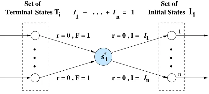
Although subtasks are episodic problems, when the overall task (root of the hierarchy) is con-tinuing as we assumed in this section (Assumption 1), they are executed an infinite number of times, and therefore can be modeled as continuing problems using the model described in Figure 4. In this model, each subtask Miterminates at one of its terminal states s∈Ti. All terminal states transit with
probability 1 and reward 0 to a dummy state s∗i. Finally, the dummy state s∗i transits with reward zero to one of the initial states (∈Ii) of subtask Mi upon the next instantiation of Mi. These are
dummy transitions and do not add any time-step to the cycle of subtask Mi and therefore are not
taken into consideration when the average reward of subtask Miis calculated. It is important for the
validity of the model to fix the value of dummy states to zero.
*
s
Terminal States
n
. . .
1.
.
.
.
.
.
1
n
Set of
T
i Initial StatesI
iSet of
r = 0 , I = In r = 0 , I = I1
I + + I = 1
i
r = 0 , F = 1
r = 0 , F = 1