Controlling the False Discovery Rate of the Association/Causality
Structure Learned with the PC Algorithm
Junning Li [email protected]
Z. Jane Wang [email protected]
Department of Electrical and Computer Engineering University of British Columbia
Vancouver, BC, V6T 1Z4 Canada
Editors: Paolo Frasconi, Kristian Kersting, Hannu Toivonen and Koji Tsuda
Abstract
In real world applications, graphical statistical models are not only a tool for operations such as classification or prediction, but usually the network structures of the models themselves are also of great interest (e.g., in modeling brain connectivity). The false discovery rate (FDR), the expected ratio of falsely claimed connections to all those claimed, is often a reasonable error-rate criterion in these applications. However, current learning algorithms for graphical models have not been adequately adapted to the concerns of the FDR. The traditional practice of controlling the type I error rate and the type II error rate under a conventional level does not necessarily keep the FDR low, especially in the case of sparse networks. In this paper, we propose embedding an FDR-control procedure into the PC algorithm to curb the FDR of the skeleton of the learned graph. We prove that the proposed method can control the FDR under a user-specified level at the limit of large sample sizes. In the cases of moderate sample size (about several hundred), empirical experiments show that the method is still able to control the FDR under the user-specified level, and a heuristic modification of the method is able to control the FDR more accurately around the user-specified level. The proposed method is applicable to any models for which statistical tests of conditional independence are available, such as discrete models and Gaussian models.
Keywords: Bayesian networks, false discovery rate, PC algorithm, directed acyclic graph,
skele-ton
1. Introduction
As a fundamental and intuitive tool to analyze and visualize the association and/or causality relationships among multiple events, graphical models have become more and more explored in biomedical researches, such as discovering gene regulatory networks and modelling functional con-nectivity between brain regions. In these real world applications, graphical models are not only a tool for operations such as classification or prediction, but often the network structures of the mod-els themselves are also output of great interest: a set of association and/or causality relationships discovered from experimental observations. For these applications, a desirable structure-learning method needs to account for the error rate of the graphical features of the discovered network. Thus, it is important for structure-learning algorithms to control the error rate of the association/causality relationships discovered from a limited number of observations closely below a user-specified level, in addition to finding a model that fits the data well. As edges are fundamental elements of a graph, error rates related to them are of natural concerns.
In a statistical decision process, there are basically two sources of errors: the type I errors, that is, falsely rejecting negative hypotheses when they are actually true; and the type II errors, that is, falsely accepting negative hypotheses when their alternatives, the positive hypotheses are actually true. In the context of learning graph structures, a negative hypothesis could be that an edge does not exist in the graph while the positive hypothesis could be that the edge does exist. Because of the stochastic nature of random sampling, data of a limited sample size may appear to support a positive hypothesis more than a negative hypothesis even when actually the negative hypothesis is true, or vice versa. Thus it is generally impossible to absolutely prevent the two types of errors simultaneously, but has to set a threshold on a certain type of errors, or keep a balance between the them, for instance by minimizing a certain lost function associated with the errors according to the Bayesian decision theory. For example, when diagnosing cancer, to catch the potential chance of saving a patient’s life, doctors probably hope that the type II error rate, that is, the probability of falsely diagnosing a cancer patient as healthy, to be low, such as less than 5%. Meanwhile, when diagnosing a disease whose treatment is so risky that may cause the loss of eyesight, to avoid the unnecessary but great risk for healthy people, doctors probably hope that the type I error rate, that is, the probability of falsely diagnosing a healthy people as affected by the disease, to be extremely low, such as less than 0.1%. Learning network structures may face scenarios similar to the two cases above of diagnosing diseases. Given data of a limited sample size, there is not an algorithm guaranteeing a perfect recovery of the structure of the underlying graphical model, and any algorithm has to compromise on the two types of errors.
The false discovery rate (FDR) (see Benjamini and Yekutieli, 2001; Storey, 2002), defined as the expected ratio of falsely discovered positive hypotheses to all those discovered, has become an important and widely used criterion in many research fields, such as bioinformatics and neuroimag-ing. In many real world applications that involve multiple hypothesis testing, the FDR is more reasonable than the traditional type I error rate and type II error rate. Suppose that in a pilot study researchers are selecting candidate genes for a genetic research on schizophrenia. Due to the limited funding, only a limited number of genes can be studied thoroughly in the afterward genetic research. To use the funding efficiently, researchers would hope that 95% of the candidate genes selected in the pilot study are truly associated with the disease. In this case, the FDR is chosen as the error rate of interest and should be controlled under 5%. Simply controlling the type I error rate and the type II error rate under certain levels does not necessarily keep the FDR sufficiently low, especially in the case of sparse networks. For example, suppose a gene regulatory network involves 100 genes, where each gene interacts in average with 3 others, that is, there are 150 edges in the network. Then an algorithm with the realized type I error rate = 5% and the realized power = 90% (i.e., the
real-ized type II error rate = 10%) will recover a network with 150×90%=135 correct connections and
[100×(100−1)/2−150]×5%=240 false connections. This means that 240/(240+135) =64% of the claimed connections actually do not exist in the true network. Due to the popularity of the FDR in research practices, it is highly desirable to develop structure-learning algorithms that allow the control over the FDR on network structures.
However, current structure-learning algorithms for Bayesian networks have not been adequately adapted to explicitly controlling the FDR of the claimed “discovered” networks. Score-based search methods (see Heckerman et al., 1995) look for a suitable structure by optimizing a certain criterion of goodness-of-fit, such as the Akaike information criterion (AIC), the Bayesian information crite-rion (BIC), or the Bayesian Dirichlet likelihood equivalent metric (BDE), with a random walk (e.g., simulated annealing) or a greedy walk (e.g., hill-climbing), in the space of DAGs or their equiva-lence classes.1 It is worth noting that the restricted case of tree-structured Bayesian networks has been optimally solved, in the sense of Kullback-Leibler divergence, with Chow and Liu (1968)’s method, and that Chickering (2002) has proved that the greedy equivalence search can identify the true equivalence class in the limit of large sample sizes. Nevertheless, scores do not directly reflect the error rate of edges, and the sample sizes in real world applications are usually not large enough to guarantee the perfect asymptotic identification.
The Bayesian approach first assumes a certain prior probability distribution over the network structures, and then estimates the posterior probability distribution of the structures after data are observed. Theoretically, the posterior probability of any structure features, such as the existence of an edge, the existence of a path, or even the existence of a sub-graph, can be estimated with the Bayesian approach. This consequently allows the control of the posterior error rate of these structure features, that is, the posterior probability of the non-existence of these features. It should be pointed out that the posterior error rate is conceptually different from those error rates such as the type I error rate, the type II error rate, and the FDR, basically because they are from different statistical perspectives. The posterior error rate is defined from the perspective of Bayesian statistics. From the Bayesian perspective, network structures are assumed to be random, according to a probability distribution, and the posterior error rate is the probability of the non-existence of certain features according to the posterior probability distribution over the network structures. Given the same data,
different posterior distributions will be derived from different prior distributions. The type I error rate, the type II error rate, and the FDR are defined from the perspective of classical statistics. From the classical perspective, there is a true, yet unknown, model behind the data, and the error rates are defined by comparing with the true model. Nevertheless, a variant of the FDR, the positive false discovery rate (pFDR) proposed by Storey (2002), can be interpreted from the Bayesian perspective (Storey, 2003).
The Bayesian approach for structure learning is usually conducted with the maximum-a
poste-riori-probability (MAP) method or the posterior-expectation method. The MAP method selects the
network structure with the largest posterior probability. The optimal structure is usually searched for in a score-based manner, with the posterior probability or more often approximations to the relative posterior probability (for instance the BIC score) being the score to optimize. Cooper and Her-skovits (1992) developed a heuristic greedy search algorithm called K22that can finish the search in a polynomial time with respect to the number of vertices, given the order of vertices. The MAP method provides us with a single network structure, the posteriorly most probable one, but does not address error rates in the Bayesian approach.
To control errors in the Bayesian approach, the network structure should be learned with the posterior-expectation method, that is, calculating the posterior probabilities of network structures, and then deriving the posterior expectation of the existence of certain structure features. Though theoretically the posterior-expectation method can control the error rate of any structure features, in practice its capacity is largely limited for computational reasons. The number of DAGs increases super-exponentially as the number of vertices increases (Robinson, 1973). For 10 vertices, there are already about 4.2×10¹⁸DAGs. Though the number of equivalence classes of DAGs is much smaller than the number of DAGs, it is still forbiddingly large, empirically asymptotically decreasing to 1/13.652 of the number of DAGs, as the number of vertices increases (Steinsky, 2003). Therefore, exact inferences of posterior probabilities are only feasible for small scale problems, or under cer-tain additional constraints. For cercer-tain prior distributions, and given the order of vertices, Friedman and Koller (2003) have derived a formula that can be used to calculate the exact posterior probabil-ity of a structure feature with the computational complexprobabil-ity bounded by O(NDin+1), where N is the
number of vertices and Dinis the upper bound of the in-degree for each vertex. Considering similar
prior distributions, but without the restriction on the order of vertices, Koivisto and Sood (2004) have developed a fast exact Bayesian inference algorithm based on dynamic programming that is able to compute the exact posterior probability of a sub-network with the computational complexity bounded by O(N2N+NDin+1L(m)), where L(m)is the complexity of computing a marginal
condi-tional likelihood from m samples. In practice, this algorithm runs fairly fast when the number of vertices is less than 25. For networks with more than 30 vertices, the authors suggested setting more restrictions or combining with inexact techniques. These two breakthroughs made exact Bayesian inferences practical for certain prior distributions. However, as Friedman and Koller (2003) pointed out, the prior distributions which facilitate the exact inference are not hypothesis equivalent (see Heckerman et al., 1995), that is, different network structures that are in the same equivalence class often have different priors. The simulation performed by Eaton and Murphy (2007) confirmed that these prior distributions deviate far from the uniform distributions. This implies that the methods cannot be applied to the widely accepted uninformative prior, that is, the uniform prior distribution over DAGs. For general problems, the posterior probability of a structure feature can be
imated with Markov chain Monte Carlo (MCMC) methods (Madigan et al., 1995). As a versatile implementation of Bayesian inferences, the MCMC method can estimate the posterior probability given any prior probability distribution. However, MCMC usually requires intensive computation and results may depend on the initial state of the randomization.
Constraint-based approaches, such as the SGS3 algorithm (see Spirtes et al., 2001, pages 82– 83), inductive causation (IC)4(see Pearl, 2000, pages 49–51), and the PC5algorithm (see Spirtes et al., 2001, pages 84–89), are rooted in the directed Markov property, the rule by which Bayesian networks encode conditional independence. These methods first test hypotheses of conditional inde-pendence among random variables, and then combine those accepted hypotheses of conditional in-dependence to construct a partially directed acyclic graph (PDAG) according to the directed Markov property. The computational complexity of these algorithms is difficult to analyze exactly, though for the worst case, which rarely occurs in real world applications, is surely bounded by O(N22N)
where N is the number of vertices. In practice, the PC algorithm and the fast-causal-inference (FCI) algorithm (see Spirtes et al., 2001, pages 142–146) can achieve polynomial time if the maximum degree of a graph is fixed. It has been proved that if the true model satisfies the faithfulness con-straints (see Spirtes et al., 2001, pages 13 and 81) and all the conditional-independence/dependence relationships are correctly identified, then the PC algorithm and the IC algorithm can exactly re-cover the true equivalence class, and so do the FCI algorithm and the IC* algorithm6 (see Pearl, 2000, pages 51–54) for problems with latent variables. Kalisch and B¨uhlmann (2007) have proved that for Gaussian Bayesian networks, the PC algorithm can consistently estimate the equivalence class of an underlying sparse DAG as the sample size m approaches infinity, even if the number of vertices N grows as fast as O(mλ)for any 0<λ<∞. Yet, as in practice hypotheses of condi-tional independence are tested with statistical inference from limited data, false decisions cannot be entirely avoided and thus the ideal recovery cannot be achieved. In current implementations of the constraint-based approaches, the error rate of testing conditional independence is usually con-trolled individually for each test, under a conventional level such as 5% or 1%, without correcting the effect of multiple hypothesis testing. Therefore these implementations may fail to curb the FDR, especially for sparse graphs.
In this paper, we propose embedding an FDR-control procedure into the PC algorithm to curb the error rate of the skeleton of the learned PDAGs. Instead of individually controlling the type I error rate of each hypothesis test, the FDR-control procedure considers the hypothesis tests to-gether to correct the effect of simultaneously testing the existence of multiple edges. We prove that the proposed method, named as the PCfdr-skeleton algorithm, can control the FDR under a
user-specified level at the limit of large sample sizes. In the case of moderate sample sizes (about several hundred), empirical experiments show that the method is able to control the FDR under the user-specified level, and a heuristic modification of the method is able to control the FDR more accu-rately around the user-specified level. Sch¨afer and Strimmer (2005) have applied an FDR procedure to graphical Gaussian models to control the FDR of the non-zero entries of the partial correlation matrix. Different from Sch¨afer and Strimmer (2005)’s work, our method, built within the
frame-3. “SGS” stands for Spirtes, Glymour and Scheines who invented this algorithm.
4. An extension of the IC algorithm which was named as IC* (see Pearl, 2000, pages 51–54) was previously also named as IC by Pearl and Verma (1992). Here we follow Pearl (2000).
5. “PC” stands for Peter Spirtes and Clark Glymour who invented this algorithm. A modified version of the PC algo-rithm which was named as PC* (see Spirtes et al., 2001, pages 89–90) was previously also named as PC by Spirtes and Glymour (1991). Here we follow Spirtes et al. (2001).
work of the PC algorithm, is not only applicable to the special case of Gaussian models, but also generally applicable to any models for which conditional-independence tests are available, such as discrete models.
We are particularly interested in the PC algorithm because it roots in conditional-independence relationships, the backbone of Bayesian networks, and p-values of hypothesis testing represent one type of error rates. We consider the skeleton of graphs because constraint-based algorithms usually first construct an undirected graph, and then annotate it into different types of graphs while keeping the skeleton as the same as that of the undirected one.
The PCfdr-skeleton algorithm is not designed to replace or claimed to be superior over the
stan-dard PC algorithm, but provide the PC algorithm with the ability to control the FDR over the skele-ton of the recovered network. The PCfdr-skeleton algorithm controls the FDR while the standard
PC algorithm controls the type I error rate, as illustrated in Section 3.1. Since there are no general superior relationships between different error-rate criteria, as explained in Appendix C, neither be there between the PCfdr-skeleton algorithm and the standard PC algorithm. In research practices,
researchers first decide which error rate is of interest, and then choose appropriate algorithms to control the error rate of interest. Generally they will not select an algorithm that sounds “superior” but controls the wrong error rate. Since the purpose of the paper is to provide the PC algorithm with the control over the FDR, we assume in this paper that the FDR has been selected as the error rate of interest, and selecting the error rate of interest is out of the scope of the paper.
The remainder of the paper is organized as follows. In Section 2, we review the PC algorithm, present the FDR-embedded PC algorithm, prove its asymptotic performance, and analyze its com-putational complexity. In Section 3, we evaluate the proposed method with simulated data, and demonstrate its real world applications to learning functional connectivity networks between brain regions using functional-magnetic-resonance-imaging (fMRI). Finally, we discuss the advantages and limitations of the proposed method in Section 4.
2. Controlling FDR with PC Algorithm
In this section, we first briefly introduce Bayesian networks and review the PC algorithm. Then, we expatiate on the FDR-embedded PC algorithm and its heuristic modification, prove their asymptotic performances, and analyze their computational complexity. At the end, we discuss other possible ideas of embedding FDR control into the PC algorithm.
2.1 Notations and Preliminaries
To assist the reading, notations frequently used in the paper are listed as follows:
a, b, ··· : vertices
Xa, Xb, ··· : variables respectively represented by vertices a, b, ··· A,B, ··· : vertex sets
XA,XB, ··· : variable sets respectively represented by vertex sets A,B, ···
V : the vertex set of a graph
N=|V| : the number of vertices of a graph
a→b : a directed edge or an ordered pair of vertices
E : a set of directed edges
E∼ : the undirected edges derived from E, that is,{a∼b|a→b or b→a∈E} G= (V,E) : a directed graph composed of vertices in V and edges in E
G∼= (V,E∼) : the skeleton of a directed graph G= (V,E)
adj(a,G) : vertices adjacent to a in graph G, that is,{b|a→b or b→a∈E}
adj(a,G∼) : vertices adjacent to a in graph G∼, that is,{b|a∼b∈E∼} a⊥b|C : vertices a and b are d-separated by vertex set C
Xa⊥Xb|XC : Xaand Xbare conditional independent given XC pa⊥b|C : the p-value of testing Xa⊥Xb|XC
A Bayesian network encodes a set of conditional-independence relationships with a DAG G= (V,E)according to the directed Markov property defined as follows.
Definition 1 the Directed Markov Property: if A and B are d-separated by C where A, B and C are three disjoint sets of vertices, then XA and XB are conditionally independent given XC, that is, P(XA,XB|XC)= P(XA|XC)P(XB|XC). (see Lauritzen, 1996, pages 46–53)
The concept of d-separation (see Lauritzen, 1996, page 48) is defined as follows. A chain between two vertices a and b is a sequence a = a0,a1, . . . ,an= b of distinct vertices such that ai−1∼ai∈E∼
for all i=1, . . . , n. Vertex b is a descendant of vertex a if and only if there is a sequence a= a0,a1, . . . ,an=b of distinct vertices such that ai−1→ai∈E for all i=1, . . . , n. For three disjoint
subsets A, B and C⊆V , C d-separates A and B if and only if any chainπbetween∀a∈A and∀b∈B
contains a vertexγ∈πsuch that either
• arrows ofπdo not meet head-to-head atγandγ∈C, or
• arrows ofπmeet head-to-head atγandγis neither in C nor has any descendants in C.
Moreover, a probability distribution P is faithful to a DAG G (see Spirtes et al., 2001, pages 13 and 81) if all and only the conditional-independence relationships derived from P are encoded by
G. In general, a probability distribution may possess other independence relationships besides those
encoded by a DAG.
It should be pointed out that there are often several different DAGs encoding the same set of conditional-independence relationships and they are called an equivalence class of DAGs. An equivalence class can be uniquely represented by a completed acyclic partially directed graph (CPDAG) (also called the essential graph in the literature) that has the same skeleton as a DAG does except that some edges are not directed (see Andersson et al., 1997).
2.2 PC Algorithm
(conventionally 5% or 1%), then the hypothesis of conditional independence is rejected while the hypothesis of conditional dependence Xa⊥Xb|XCis accepted.
The first step of the PC algorithm is to construct an undirected graph G∼ whose edge direc-tions will later be further determined with other steps, while the skeleton is kept the same as that of G∼. Since we restrict ourselves to the error rate of the skeleton, here we only present in Al-gorithm 1 the first step of the PC alAl-gorithm, as implemented in software Tetrad version 4.3.8 (see http://www.phil.cmu.edu/projects/tetrad), and refer to it as the PC-skeleton algorithm.
Algorithm 1 PC-skeleton
Input: the data XV generated from a probability distribution faithful to a DAG Gtrue,
and the significance levelαfor every statistical test of conditional independence Output: the recovered skeleton G∼
1: Form the complete undirected graph G∼on the vertex set V .
2: Let depth d = 0.
3: repeat
4: for each ordered pair of adjacent vertices a and b in G∼, that is, a∼b∈E∼do
5: if|adj(a,G∼)\ {b}| ≥d, then
6: for each subset C⊆adj(a,G∼)\ {b}and|C|=d do
7: Test hypothesis Xa⊥Xb|XCand calculate the p-value pa⊥b|C.
8: if pa⊥b|C≥α, then
9: Remove edge a∼b from G∼.
10: Update G∼and E∼.
11: break the for loop at line 6
12: end if
13: end for
14: end if
15: end for
16: Let d=d+1.
17: until|adj(a,G∼)\ {b}|<d for every ordered pair of adjacent vertices a and b in G∼.
The theoretical foundation of the PC-skeleton algorithm is Proposition 1: if two vertices a and
b are not adjacent in a DAG G, then there is a set of other vertices C that either all are neighbors of a or all are neighbors of b such that C d-separates a and b, or equivalently, Xa⊥Xb|XC, according to
the directed Markov property. Since two adjacent vertices are not d-separated by any set of other vertices (according to the directed Markov property), Proposition 1 implies that a and b are not adjacent if and only if there is a d-separating C in either neighbors of a or neighbors of b. Readers should notice that the proposition does not imply that a and b are d-separated only by such a C, but just guarantees that a d-separating C can be found in either neighbors of a or neighbors b.
Proposition 1 If vertices a and b are not adjacent in a DAG G, then there is a set of vertices C which is either a subset of adj(a,G)\ {b} or a subset of adj(b,G)\ {a} such that C d-separates a and b in G. This proposition is a corollary of Lemma 5.1.1 on page 411 of book Causation,
The logic of the PC-skeleton algorithm is as follows, under the assumption of perfect judgment on conditional independence. The most straightforward application of Proposition 1 to structure learning is to exhaustively search all the possible neighbors of a and b to verify whether there is such a d-separating C to disconnect a and b. Since the possible neighbors of a and b are unknown, to guarantee the detection of such a d-separating C, all the vertices other than a and b should be searched as possible neighbors of a and b. However, such a straightforward application is very inefficient because it probably searches many unnecessary combinations of vertices by considering all the vertices other than a and b as their possible neighbors, especially when the true DAG is sparse. The PC-skeleton algorithm searches more efficiently, by keeping updating the possible neighbors of a vertex once some previously-considered possible neighbors have been found actually not connected with the vertex. Starting with a fully connected undirected graph G∼ (step 1), the algorithm searches for the d-separating C progressively by increasing the size of C, that is, the number of conditional variables, from zero (step 2) with the step size of one (step 16). Given the size of C, the search is performed for every vertex pair a and b (step 4). Once a C d-separating a and b is found (step 8), a and b are disconnected (step 9), and the neighbors of a and b are updated (step 10). In the algorithm, G∼ is continually updated, so adj(a,G∼) is also constantly updated as the algorithm progresses. The algorithm stops when all the subsets of the current neighbors of each vertex have been examined (step 17). The Tetrad implementation of the PC-skeleton algorithm examines an edge a∼b as two ordered pairs (a, b) and (b, a) (step 4), each time searching for
the d-separating C in the neighbors of the first element of the pair (step 6). In this way, both the neighbors of a and the neighbors of b are explored.
The accuracy of the PC-skeleton algorithm depends on the discriminability of the statistical test of conditional independence. If the test can perfectly distinguish dependence from independence, then the algorithm can correctly recover the true underlying skeleton, as proved by Spirtes et al. (2001, pages 410–412). The outline of the proof is as follows. First, all the true edges will be recovered because an adjacent vertex pair a∼b is not d-separated by any vertex set C that excludes a and b. Second, if the edge between a non-adjacent vertex pair a and b has not been removed,
subsets of either adj(a,G)\ {b}or adj(b,G)\ {a}will be searched until the C that d-separates a and
b according to Proposition 1 is found, and consequently the edge between a and b will be removed.
If the judgments on conditional independence and conditional dependence are imperfect, the PC-skeleton algorithm is unstable. If an edge is mistakenly removed from the graph in the early stage of the algorithm, then other edges which are not in the true graph may be included in the graph (see Spirtes et al., 2001, page 87).
2.3 False Discovery Rate
Test Results Truth
Negative Positive Total
Negative TN (true negative) FN (false negative) R1
Positive FP (false positive) TP (true positive) R2
Total T1 T2
Table 1: Results of multiple hypothesis testing, categorized according to the claimed results and the truth.
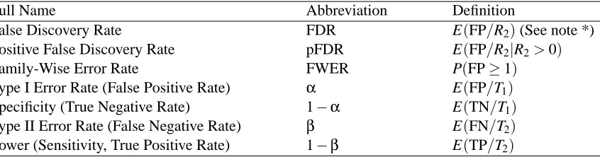
Full Name Abbreviation Definition
False Discovery Rate FDR E(FP/R2)(See note *)
Positive False Discovery Rate pFDR E(FP/R2|R2>0)
Family-Wise Error Rate FWER P(FP≥1)
Type I Error Rate (False Positive Rate) α E(FP/T1)
Specificity (True Negative Rate) 1−α E(TN/T1)
Type II Error Rate (False Negative Rate) β E(FN/T2)
Power (Sensitivity, True Positive Rate) 1−β E(TP/T2)
Table 2: Criteria for multiple hypothesis testing. Here E(x) means the expected value of x, and
P(
A
)means the probability of eventA
. Please refer to Table 1 for related notations. * IfR2=0, FP/R2is defined to be 0.
The FDR is a reasonable criterion when researchers expect the “discovered” results are trustful and dependable in afterward studies. For example, in a pilot study, we are selecting candidate genes for a genetic research on Parkinson’s disease. Because of the limited funding, we can only study a limited number of genes in the afterward genetic research. Thus, when selecting candidate genes in the pilot study, we hope that 95% of the selected candidate genes are truly associated with the disease. In this case, the FDR is chosen as the error rate of interest and should be controlled under 5%. Since similar situations are quite common in research practices, the FDR has been widely adopted in many research fields such as bioinformatics and neuroimaging.
In the context of learning the skeleton of a DAG, a negative hypothesis could be that a connection does not exist in the DAG, and a positive hypothesis could be that the connection exists. The FDR is the expected proportion of the falsely discovered connections to all those discovered. Learning network structures may face scenarios similar to the aforementioned pilot study, but the FDR control has not yet received adequate attention in structure learning.
realized FDR of a trial under q, but control the expected value of the error rate when the procedures
are repetitively applied to randomly sampled data.
Algorithm 2 FDR-stepup
Input: a set of p-values{pi|i=1, . . . ,H}, and the threshold of the FDR q
Output: the set of rejected null hypotheses
1: Sort the p-values of H hypothesis tests in the ascendant order as p(1)≤. . .≤p(H).
2: Let i=H, and H∗=H (or H∗=H(1+1/2, . . . ,+1/H), depending on the assumption of the dependency among the test statistics).
3: while
H∗
i p(i)>q and i>0, (1) do
4: Let i=i−1.
5: end while
6: Reject the null hypotheses associated with p(1), . . . ,p(i), and accept the null hypotheses associ-ated with p(i+1), . . . ,p(H).
Besides the FDR and the pFDR, other criteria, as listed in Table 2, can also be applied to assess the uncertainty of multiple hypothesis testing. The type I error rate is the expected ratio of the type I errors to all the negative hypotheses that are actually true. The type II error rate is the expected ratio of the type II errors to all the positive hypotheses that are actually true. The family-wise error rate is the probability that at least one of the accepted positive hypotheses are actually wrong. Generally, there are not mathematically or technically superior relationships among these error-rate criteria. Please refer to Appendix C for examples of typical research scenarios where each particular error rate is favoured.
Controlling both the type I and the type II error rates under a conventional level (such asα< 5% or 1% andβ<10% or 5%) does not necessarily curb the FDR at a desired level. As shown in Eq. (2), if FP/T1 and FN/T2 are fixed and positive, FP/R2 approaches 1 when T2/T1 is small
enough. This is the case of sparse networks where the number of existing connections T2is much
smaller than the number of non-existing connections T1.
FP
R2 =
FP T1
FP T1 + (1−
FN T2)
T2
T 1
. (2)
2.4 PC Algorithm with FDR
algorithm. Similar to the PC-skeleton algorithm, G∼, adj(a,G∼)and E∼are constantly updated as the algorithm progresses.
The PCfdr-skeleton and the PC-skeleton algorithms share the same search strategy, but differ
on the judgment of conditional independence. The same as the PC-skeleton algorithm, the PCfdr
-skeleton algorithm increases d, the number of conditional variables, from zero (step 3) with the step size of one (step 25), and also keeps updating the neighbors of vertices (steps 14 and 15) when some previously-considered possible neighbors have been considered not connected (step 13). The PCfdr
-skeleton algorithm differs from the PC--skeleton algorithm on the inference of d-separation, with its steps 11–20 replacing steps 8–12 of the PC-skeleton algorithm. In the PC-skeleton algorithm, two vertices are regarded as d-separated once the conditional-independence test between them yields a
p-value larger than the pre-defined significant levelα. In this way, the type I error of each statistical test is controlled separately, without consideration of the effect of multiple hypothesis testing. The PCfdr-skeleton algorithm records in pmaxa∼bthe up-to-date maximum p-value associated with an edge a∼b (steps 9 and 10), and progressively removes those edges whose non-existence is accepted
by the FDR procedure (step 12), with Pmax = {pmaxa∼b}a6=b and the pre-defined FDR level q being
the input. The FDR procedure, Algorithm 2, is invoked at step 12, either immediately after every element of Pmax has been assigned a valid p-value for the first time, or later once any element of
Pmaxis updated.
The pmaxa∼bis the upper bound of the p-value of testing the hypothesis that a and b are d-separated by at least one of the vertex sets C searched in step 7. According to the directed Markov property, a and b are not adjacent if and only if there is a set of vertices C⊆V\ {a,b}d-separating a and b. As the algorithm progresses, the d-separations between a and b by vertex sets C1, . . . ,CK ⊆V\ {a,b}
are tested respectively, and consequently a sequence of p-values p1, . . . ,pKare calculated. If we use pmaxa∼b=maxKi=1pi as the statistic to test the negative hypothesis that there is, though unknown, a Cj
among C1, . . . ,CKd-separating a and b, then due to P(pmax
a∼b≤p) =P(pi≤p for all i=1, . . . ,K)≤P(pj≤p) =p, (3) pmaxa∼bis the upper bound of the p-value of testing the negative hypothesis. Eq. (3) also clearly shows that the PC-skeleton algorithm controls the type I error rate of the negative hypothesis, since its step 8 is equivalent to “if pmaxa∼b<α, then . . . ” if pmaxa∼bis recorded in the PC-skeleton algorithm.
The statistical tests performed at step 8 of the PCfdr-skeleton algorithm generally are not
in-dependent with each other, since the variables involved in two hypotheses of conditional indepen-dence may overlap. For example, conditional-indepenindepen-dence relationships a⊥b1|C and a⊥b2|C both
involve a and C. It is very difficult to prove whether elements of Pmax have positive regression dependency or not, so rigorously the conservative modification of Algorithm 2, should be applied at step 12. However, since pmaxa∼bis probably a loose upper bound of the p-value of testing a≁b, in
practice we simply apply the FDR procedure that is correct for positive regression dependency. It should be noted that different from step 9 of the PC-skeleton algorithm, step 14 of the PCfdr
-skeleton algorithm may remove edges other than just a∼b, because the decisions on other edges
can be affected by the updating of pmax a∼b.
A heuristic modification of the PCfdr-skeleton algorithm is to remove pmaxa∼b from Pmax once
edge a∼b has been deleted from G∼ at step 14. We name this modified version as the PCfdr*
-skeleton algorithm. In the PCfdr-skeleton algorithm, pmaxa∼bis still recorded in Pmaxand input to the
FDR procedure after the edge a∼b has been removed. This guarantees that the algorithm can
Algorithm 3 PCfdr-skeleton
Input: the data XV generated from a probability distribution faithful to a DAG Gtrue,
and the FDR level q for the discovered skeleton Output: the recovered skeleton G∼
1: Form the complete undirected graph G∼on the vertex set V
2: Initialize the maximum p-values associated with edges as
Pmax={pmaxa∼b=−1}a6=b.
3: Let depth d = 0.
4: repeat
5: for each ordered pair of adjacent vertices a and b in G∼, that is, a∼b∈E∼do
6: if |adj(a,G∼)\ {b}| ≥d, then
7: for each subset C⊆adj(a,G∼)\ {b}and|C|=d do
8: Test hypothesis Xa⊥Xb|XCand calculate the p-value pa⊥b|C.
9: if pa⊥b|C>pmaxa∼b, then
10: Let pmaxa∼b=pa⊥b|C.
11: if every element of Pmaxhas been assigned a valid p-value by step 10, then
12: Run the FDR procedure, Algorithm 2, with Pmaxand q as the input.
13: if the non-existence of certain edges are accepted, then
14: Remove these edges from G∼.
15: Update G∼and E∼.
16: if a∼b is removed, then
17: break the for loop at line 7.
18: end if
19: end if
20: end if
21: end if
22: end for
23: end if
24: end for
25: Let d=d+1.
26: until|adj(a,G∼)\ {b}|<d for every ordered pair of adjacent vertices a and b in G∼.
* A heuristic modification at step 15 of the algorithm is to remove from Pmaxthe pmaxa∼bs whose asso-ciated edges have been deleted from G∼at step 14, that is, to update Pmaxas Pmax={pamax∼b}a∼b∈E∼
right after updating E∼ at step 15. This heuristic modification is named as the PCfdr*-skeleton algorithm.
2.5 Asymptotic Performance
Here we prove that the PCfdr-skeleton algorithm is able to control the FDR under a user-specified
level q (q>0) at the limit of large sample sizes if the following assumptions are satisfied:
(A1) The probability distribution P is faithful to a DAG Gtrue.
(A2) The number of vertices is fixed.
(A3) Given a fixed significant level of testing conditional-independence relationships, the power of detecting conditional-dependence relationships with statistical tests approaches 1 at the limit of large sample sizes. (For the definition of power in hypothesis testing, please refer to Table 2.)
Assumption (A1) is generally assumed when graphical models are applied, although it restricts the probability distribution P to a certain class. Assumption (A2) is usually implicitly stated, but here we explicitly emphasize it because it simplifies the proof. Assumption (A3) may seem demanding, but actually it can be easily satisfied by standard statistical tests, such as the likelihood-ratio test introduced by Neyman and Pearson (1928), if the data are identically and independently sampled. Two statistical tests that satisfy Assumption (A3) are listed in Appendix B.
The detection power and the FDR of the PCfdr-skeleton algorithm and its heuristic modification
at the limit of large sample sizes are elucidated in Theorems 1 and 2. The detailed proofs are provided in Appendix A.
Theorem 1 Assuming (A1), (A2) and (A3), both the PCfdr-skeleton algorithm and its heuristic mod-ification, the PCfdr*-skeleton algorithm, are able to recover all the true connections with probability one as the sample size approaches infinity:
lim
m→∞P(E ∼
true⊆E∼) =1,
where Etrue∼ denotes the set of the undirected edges derived from the true DAG Gtrue, E∼denotes the set of the undirected edges recovered with the algorithms, and m denotes the sample size.
Theorem 2 Assuming (A1), (A2) and (A3), the FDR of the undirected edges recovered with the PCfdr-skeleton algorithm approaches a value not larger than the user-specified level q as the sample size m approaches infinity:
lim sup
m→∞ FDR(E ∼,E∼
true)≤q, where FDR(E∼,E∼
true)is defined as
FDR(E∼,Etrue∼ ) = E
h
|E∼\Etrue∼ | |E∼|
i
,
Define |E∼\Etrue∼ |
|E∼| = 0, if|E∼|=0.
2.6 Computational Complexity
The PCfdr-skeleton algorithm spends most of its computation on performing statistical tests of
all the other parts of both algorithms employ the same search strategy, the computation spent by the PCfdr-skeleton algorithm on statistical tests has the same complexity as that by the PC-skeleton
algorithm. The only extra computational cost of the PCfdr-skeleton algorithm is at step 12 for
con-trolling the FDR.
The computational complexity of the search strategy employed by the PC algorithm has been studied by Kalisch and B¨uhlmann (2007) and Spirtes et al. (see 2001, pages 85–87). Here to make the paper self-contained, we briefly summarize the results as follows. It is difficult to analyze the complexity exactly, but if the algorithm stops at the depth d=dmax, then the number of
conditional-independence tests required is bounded by
T=2C2N
dmax
∑
d=0 CNd−2,
where N is the number of vertices, CN2 is the number of combinations of choosing 2 un-ordered and distinct elements from N elements, and similarly CN2−2is the number of combinations of choosing from N−2 elements. In the worst case that dmax=N−2, the complexity is bounded by 2C2N2N−2.
The bound usually is very loose, because it assumes that no edge has been removed until d=dmax.
In real world applications, the algorithm is very fast for sparse networks.
The computational complexity of the FDR procedure, Algorithm 2, generally is O( H log(H)
+ H) = O(H log(H))where H=CN2 is the number of input p-values. The sorting at step 1 costs
H log(H) and the “while” loop from step 3 to step 5 repeats H times at most. However, if the sorted Pmax is recorded during the computation, each time when an element of Pmax is updated at step 10 of the PCfdr-skeleton algorithm, the complexity of keeping the updated Pmaxsorted is only O(H). With this optimization, the complexity of the FDR-control procedure is O(H log(H))at its first operation, and is O(H)later. The FDR procedure is invoked only when pa⊥b|C>pmaxa∼b. In the
worst case that pa⊥b|C is always larger than pmaxa∼b, the complexity of the computation spent on the
FDR control in total is bounded by O(C2
Nlog(CN2) +TCN2)= O(N2log(N) +T N2)where T is the
number of performed conditional-independence tests. This is a very loose bound because it is rare that pa⊥b|Cis always larger than pmaxa∼b.
The computational complexity of the heuristic modification, the PCfdr*-skeleton algorithm, is
the same as that of the PCfdr-skeleton algorithm, since they share the same search strategy and both
employ the FDR procedure. In the PCfdr*-skeleton algorithm, the size of Pmaxkeeps decreasing as
the algorithm progresses, so each operation of the FDR procedure is more efficient. However, since the PCfdr*-skeleton algorithm adjusts the effect of multiple hypothesis testing less conservatively,
it may remove less edges than the PCfdr-skeleton algorithm does, and invokes more
conditional-independence tests. Nevertheless, their complexity is bounded by the same limit in the worst case. It is unfair to directly compare the computational time of the PCfdr-skeleton algorithm against
that of the PC-skeleton algorithm, because if the q of the former is set at the same value as theαof the latter, the former will remove more edges and perform much less statistical tests, due to its more stringent control over the type I error rate. A reasonable way is to compare the time spent on the FDR control at step 12 against that on conditional-independence tests at step 8 in each run of the PCfdr-skeleton algorithm. If Pmaxis kept sorted during the learning process as aforementioned, then
structure learning. In our simulation study in Section 3.1, the extra computation added by the FDR control was only a tiny portion, less than 0.5%, to that spent on testing conditional independence, performed with the Cochran-Mantel-Haenszel (CMH) test (see Agresti, 2002, pages 231–232), as shown in Tables 3 and 4.
2.7 Miscellaneous Discussions Discussions
An intuitive and attracting idea of adapting the PC-skeleton algorithm to the FDR control is to “smartly” determine such an appropriate threshold of the type I error rateαthat will let the errors be controlled at the pre-defined FDR level q. Given a particular problem, it is very likely that the FDR of the graphs learned by the PC-skeleton algorithm is an monotonically increasing function of the pre-defined thresholdαof the type I error rate. If this hypothesis is true, then there is a one-to-one mapping betweenαand q for the particular problem. Though we cannot prove this hypothesis rigorously, the following argument may be enlightening. Instead of directly focusing on FDR =
E(FP/R2)(see Table 2), the expected ratio of the number of false positives (FP) to the number of accepted positive hypotheses (R2), we first focus on E(FP)/E(R2), the ratio of the expected number
of false positives to the expected number of accepted positive hypotheses, since the latter is easier to link with the type I error rate according to Eq. (2), as shown in Eq. (4),
E(FP) E(R2) =
EFPT
1
EFPT
1 + (1−
FN T2 )
T2
T 1
=
EFPT
1
EFPT
1
+1−EFNT
2
T2
T1
= α
α+ (1−β)T2
T1
, (4)
whereαandβare the type I error rate and the type II error rate respectively. A sufficient condition for E(FP)/E(R2) being a monotonically increasing function of the type I error rate includes (I)
(1−β)/α>∂(1−β)/∂α, (II) T1>0 and (III) T2>0, where∂(1−β)/∂αis the derivative of(1−β)
overα. If(1−β), regarded as a function ofα, is a concave curve from (0, 0) to (1,1), then condition (I) is satisfied. Recall that(1−β)versusα actually is the receiver operating characteristic (ROC) curve, and that with an appropriate statistic the ROC curve of a hypothesis test is usually a concave curve from (0, 0) to (1,1), we speculate that condition (I) is not difficult to satisfy. With the other two mild conditions (II) T1>0 and (III) T2>0, we could expect that E(FP)/E(R2)is a monotonically
increasing function ofα. E(FP)/E(R2)is the ratio of the expected values of two random variables,
while E(FP/R2)is the expected value of the ratio of two random variables. Generally, there is not a
monotonic relationship between E(FP)/E(R2)and E(FP/R2). Nevertheless, if the average number of false positives, E(FP), increases proportionally faster than that of the accepted positives, E(R2),
we speculate that under certain conditions, the FDR = E(FP/R2)also increases accordingly. Thus
the FDR may be a monotonically increasing function of the thresholdαof the type I error rate for the PC-skeleton algorithm.
However, even though the FDR of the PC-skeleton algorithm may decrease as the pre-defined significant levelαdecreases, the FDR of the PC-skeleton algorithm still cannot be controlled at the user-specified level for general problems by “smartly” choosing anαbeforehand, but somehow has to be controlled in a slightly different way, such as the PCfdr-skeleton algorithm does. First, the
value of such an αfor the FDR control depends on the true graph, but unfortunately the graph is unknown in problems of structure learning. According to Eq. (2), the realized FDR is a function of the realized type I and type II error rates, as well as T2/T1, which in the context of structure learning
T2/T1is unknown, such anαcannot be determined completely in advance without any information about the true graph, but has to be estimated practically from the observed data. Secondly, the FDR method we employ is such a method that estimates theα from the data to control the FDR of multiple hypothesis testing. The output of the FDR algorithm is the rejection of those null hypotheses associated with p-values p(1), . . . , p(i) (see Algorithm 2). Given p(1) ≤. . .≤p(H),
the output is equivalent to the rejection of all those hypotheses whose p-values are smaller than or equal to p(i). In other words, it is equivalent to settingα=p(i)in the particular multiple hypothesis testing. Thirdly, the PCfdr-skeleton algorithm is a valid solution to combining the FDR method with
the PC-skeleton algorithm. Because the estimation of theαdepends on p-values, and p-values are calculated one by one as the PC-skeleton algorithm progresses with hypothesis tests, theαcannot be estimated separately before the PC-skeleton algorithm starts running, but the estimation has to be embedded within the algorithm, like in the PCfdr-skeleton algorithm.
Another idea on the FDR control in structure learning is a two-stage algorithm. The first stage is to draft a graph that correctly includes all the existing edges and their orientations but may also include non-existing edges as well. The second stage is to select the real parents for each vertex, with the FDR controlled, from the set of potential parents determined in the first stage. The advan-tage of this algorithm is that the selection of real parent vertices in the second sadvan-tage is completely decoupled from the determination of edge orientations, because all the parents of each vertex have been correctly connected with the particular vertex in the first stage. However, a few concerns about the algorithm should be noticed before researchers start developing this two-stage algorithm. First, to avoid missing many existing edges in the first stage, a considerable number of non-existing edges may have to be included. To guarantee a perfect protection of the existing edges given any ran-domly sampled data, the first stage must output a graph whose skeleton is a fully connected graph. The reason for this is that the type I error rate and the type II error rate contradict each other and the latter reaches zero generally when the former approaches one (see Appendix C). Rather than protecting existing edges perfectly, the first stage should trade off between the type I and the type II errors, in favour of keeping the type II error rate low. Second, selecting parent vertices from a set of candidate vertices in the second stage, in certain sense, can be regarded as learning the structure of a sub-graph locally, in which error-rate control remains as a crucial problem. Thus erro-rate control is still involved in both of the two stages. Though this two-stage idea may not essentially reduce the problem of the FDR control to an easier task, it may break the big task of simultaneously learning all edges to many local structure-learning tasks.
3. Empirical Evaluation
The PCfdr-skeleton algorithm and its heuristic modification are evaluated with simulated data sets,
in comparison with the PC-skeleton algorithm, in the sense of the FDR, the type I error rate and the power. The PCfdr-skeleton and the PC-skeleton algorithms are also applied to two real
functional-magnetic-resonance-imaging (fMRI) data sets, to check whether the two algorithms correctly curb the error rates that they are supposed to control in real world applications.
3.1 Simulation Study
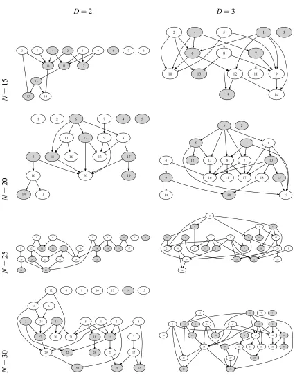
(1) Sample N×2D undirected edges from{a∼b|a,b∈V and a6=b}with equal probabilities and without replacement to compose an undirected graph G∼true.
(2) Generate a random order≻of vertices with permutation.
(3) Orientate the edges of G∼ according to the order ≻. If a is before b in the order ≻, then orientate the edge a∼b as a→b. Denote the orientated graph as a DAG Gtrue.
For each DAG, we associate its vertices with (conditional) binary probability distributions as follows, to extend it to a Bayesian network.
(1) Specify the strength of (conditional) dependence as a parameterδ>0.
(2) Randomly assign each vertex a∈V with a dependence strength δa = 0.5δ or−0.5δ, with
equal possibilities.
(3) Associate each vertex a∈V with a logistic regression model
∆=
∑
b∈pa[a] Xbδb,
P(Xa=1|Xpa[a]) =
exp(∆)
1+exp(∆),
P(Xa=−1|Xpa[a]) =
1 1+exp(∆),
where pa[a]denotes the parent vertices of a.
The parameterδ reflects the strength of dependence because if the values of all the other parent variables are fixed, the difference between the conditional probabilities of a variable Xa= 1 given a
parent variable Xb= 1 and -1 is
logit[P(Xa=1|Xb=1,Xpa[a]\{b})]−logit[P(Xa=1|Xb=−1,Xpa[a]\{b})]
=|2δb|=δ,
where the logit function is defined as logit(x) =log( x 1−x).
D=2 D=3 N = 1 5 1 11 12 2 10 3 15 4
5 9 6 7 8
14 13 1 6 9 12 14 2 10 13 3 4 7 5 8 11 15 N = 2 0 1 2 3 10 20 4 5 6 8 11 12 18 7 9 13 17 14 15 16 19 1 7 8 19 2 3 5 6 13 4 9 16 12 10 17 11 14 20 15 18 N = 2 5 1 19 2 3 15 22 24 4 5 13 17 6 14 18 7 25 8 11 12 9 16 10 20 23 21 1 7 10 15 2 9 12 13 21 3 11 22 23 4 8 5 6 14 17 19 24 20 16 18 25 N = 3 0 1 19 21 2 29 30 3 22 27 4 5 18 6 24 7 17 8 23 9 10 11 20 12 16
13 14 15
28 26 25 1 18 2 11 17 19 3 14 24 25 4 15 5 16 26 29 6 7 8 12 13 30 9 10 20 23 22 28 21 27
0.5 = logit( 0.5622 ) - logit( 0.4378 ), 0.6 = logit( 0.5744 ) - logit( 0.4256 ), 0.7 = logit( 0.5866 ) - logit( 0.4134 ), 0.8 = logit( 0.5987 ) - logit( 0.4013 ), 0.9 = logit( 0.6106 ) - logit( 0.3894 ), 1.0 = logit( 0.6225 ) - logit( 0.3775 ).
.
In total, we performed the simulation with 48 Bayesian networks generated with all the combi-nations of the following parameters:
N = 15,20,25,30;
D = 2,3;
δ = 0.5,0.6,0.7,0.8,0.9,1.0.
From each Bayesian network, we repetitively generated 50 data sets each of 500 samples to es-timate the statistical performances of the algorithms. A non-model-based test, the Cochran-Mantel-Haenszel (CMH) test (see Agresti, 2002, pages 231–232), was employed to the test conditional independence among random variables. Both the significant levelαof the PC-skeleton algorithm and the FDR level q of the PCfdr-skeleton algorithm and its heuristic modification were set at 5%.
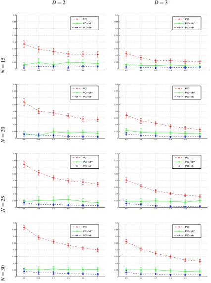
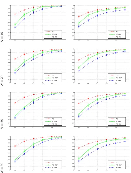
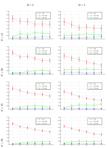
Figures 2, 3 and 4 respectively show the empirical FDR, power and type I error rate of the al-gorithms, estimated from the 50 data sets repetitively generated from each Bayesian network, with error bars indicating the 95% confidence intervals of these estimations. The PCfdr-skeleton
algo-rithm controls the FDR under the user-specified level 5% for all the 48 Bayesian networks, and the PCfdr*-skeleton algorithm steadily controls the FDR closely around 5%, while the PC-skeleton
algorithm yields the FDR ranging from about 5% to about 35%, and above 15% in many cases, especially for those sparser DAGs with the average degree of vertices D=2. The PCfdr-skeleton
al-gorithm is conservative, with the FDR notably lower than the user-specified level, while its heuristic modification controls the FDR more accurately around the user-specified level, although the correct-ness of the heuristic modification has not been theoretically proved. As the discriminability of the statistical tests increases, the power of all the algorithms approaches 1. When their FDR level q is set at the same value as theα of the PC-skeleton algorithm, the PCfdr-skeleton algorithm and its
heuristic modification control the type I error rate more stringently than the PC-skeleton algorithm does, so their power generally is lower than that of the PC-skeleton algorithm. Figure 4 also clearly shows, as Eq. 3 implies, that it is the type I error rate, rather than the FDR, that the PC-skeleton algorithm controls under 5%.
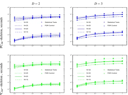
Figure 5 shows the average computational time spent during each run of the PCfdr-skeleton
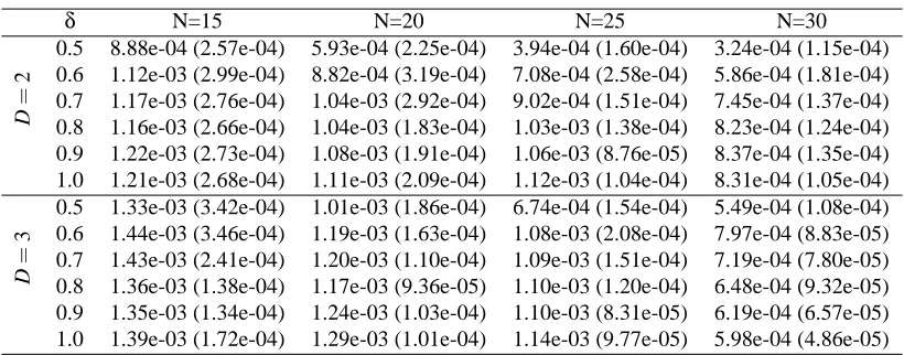
al-gorithm and its heuristic modification on the statistical tests of (conditional) independence at step 8 and the FDR control at step 12. The computational time was estimated on the platform of an Intel Xeon 1.86GHz CPU and 4G RAM, and with the code implemented in Matlab R14. Tables 3 and 4 show the average ratios of the computational time spent on the FDR control to that spent on the statistical tests. The average ratios are not more than 2.57‰ for all the 48 Bayesian networks. The relatively small standard deviations, as shown in brackets in the tables, indicate that these estimated ratios are trustful. Because the PCfdr-skeleton algorithm and its heuristic modification employ the
D=2 D=3
N
=
1
5
0.5 0.6 0.7 0.8 0.9 1
0 0.05 0.1 0.15 0.2 0.25 0.3 0.35 0.4 PC PC−fdr* PC−fdr
0.5 0.6 0.7 0.8 0.9 1
0 0.05 0.1 0.15 0.2 0.25 0.3 0.35 0.4 PC PC−fdr* PC−fdr N = 2 0
0.5 0.6 0.7 0.8 0.9 1
0 0.05 0.1 0.15 0.2 0.25 0.3 0.35 0.4 PC PC−fdr* PC−fdr
0.5 0.6 0.7 0.8 0.9 1
0 0.05 0.1 0.15 0.2 0.25 0.3 0.35 0.4 PC PC−fdr* PC−fdr N = 2 5
0.5 0.6 0.7 0.8 0.9 1
0 0.05 0.1 0.15 0.2 0.25 0.3 0.35 0.4 PC PC−fdr* PC−fdr
0.5 0.6 0.7 0.8 0.9 1
0 0.05 0.1 0.15 0.2 0.25 0.3 0.35 0.4 PC PC−fdr* PC−fdr N = 3 0
0.5 0.6 0.7 0.8 0.9 1
0 0.05 0.1 0.15 0.2 0.25 0.3 0.35 0.4 PC PC−fdr* PC−fdr
0.5 0.6 0.7 0.8 0.9 1
0 0.05 0.1 0.15 0.2 0.25 0.3 0.35 0.4 PC PC−fdr* PC−fdr
Figure 2: The FDR (with 95% confidence intervals) of the PC-skeleton algorithm, the PCfdr
-skeleton algorithm and the PCfdr*-skeleton algorithm on the DAGs in Figure 1, as the
D=2 D=3
N
=
1
5
0.5 0.6 0.7 0.8 0.9 1
0 0.1 0.2 0.3 0.4 0.5 0.6 0.7 0.8 0.9 1 PC PC−fdr* PC−fdr
0.5 0.6 0.7 0.8 0.9 1
0 0.1 0.2 0.3 0.4 0.5 0.6 0.7 0.8 0.9 1 PC PC−fdr* PC−fdr N = 2 0
0.5 0.6 0.7 0.8 0.9 1
0 0.1 0.2 0.3 0.4 0.5 0.6 0.7 0.8 0.9 1 PC PC−fdr* PC−fdr
0.5 0.6 0.7 0.8 0.9 1
0 0.1 0.2 0.3 0.4 0.5 0.6 0.7 0.8 0.9 1 PC PC−fdr* PC−fdr N = 2 5
0.5 0.6 0.7 0.8 0.9 1
0 0.1 0.2 0.3 0.4 0.5 0.6 0.7 0.8 0.9 1 PC PC−fdr* PC−fdr
0.5 0.6 0.7 0.8 0.9 1
0 0.1 0.2 0.3 0.4 0.5 0.6 0.7 0.8 0.9 1 PC PC−fdr* PC−fdr N = 3 0
0.5 0.6 0.7 0.8 0.9 1
0 0.1 0.2 0.3 0.4 0.5 0.6 0.7 0.8 0.9 1 PC PC−fdr* PC−fdr
0.5 0.6 0.7 0.8 0.9 1
0 0.1 0.2 0.3 0.4 0.5 0.6 0.7 0.8 0.9 1 PC PC−fdr* PC−fdr
Figure 3: The power (with 95% confidence intervals) of the PC-skeleton algorithm, the PCfdr
-skeleton algorithm and the PCfdr*-skeleton algorithm on the DAGs in Figure 1, as the
D=2 D=3
N
=
1
5
0.5 0.6 0.7 0.8 0.9 1
0 0.005 0.01 0.015 0.02 0.025 0.03 0.035 0.04 PC PC−fdr* PC−fdr
0.5 0.6 0.7 0.8 0.9 1
0 0.005 0.01 0.015 0.02 0.025 0.03 0.035 0.04 PC PC−fdr* PC−fdr N = 2 0
0.5 0.6 0.7 0.8 0.9 1
0 0.005 0.01 0.015 0.02 0.025 0.03 0.035 0.04 PC PC−fdr* PC−fdr
0.5 0.6 0.7 0.8 0.9 1
0 0.005 0.01 0.015 0.02 0.025 0.03 0.035 0.04 PC PC−fdr* PC−fdr N = 2 5
0.5 0.6 0.7 0.8 0.9 1
0 0.005 0.01 0.015 0.02 0.025 0.03 0.035 0.04 PC PC−fdr* PC−fdr
0.5 0.6 0.7 0.8 0.9 1
0 0.005 0.01 0.015 0.02 0.025 0.03 0.035 0.04 PC PC−fdr* PC−fdr N = 3 0
0.5 0.6 0.7 0.8 0.9 1
0 0.005 0.01 0.015 0.02 0.025 0.03 0.035 0.04 PC PC−fdr* PC−fdr
0.5 0.6 0.7 0.8 0.9 1
0 0.005 0.01 0.015 0.02 0.025 0.03 0.035 0.04 PC PC−fdr* PC−fdr
Figure 4: The type I error rates (with 95% confidence intervals) of the PC-skeleton algorithm, the PCfdr-skeleton algorithm and the PCfdr*-skeleton algorithm on the DAGs in Figure 1, as
D=2 D=3 P Cfd r -s k ele to n , se co n d s
0.5 0.6 0.7 0.8 0.9 1 10−3 10−2 10−1 100 101 102 N=15 N=20 N=25 N=30 FDR Control Statistical Tests
0.5 0.6 0.7 0.8 0.9 1 10−3 10−2 10−1 100 101 102 N=15 N=20 N=25 N=30 FDR Control Statistical Tests P Cfd r* -s k ele to n , se co n d s
0.5 0.6 0.7 0.8 0.9 1 10−3 10−2 10−1 100 101 102 N=15 N=20 N=25 N=30 FDR Control Statistical Tests
0.5 0.6 0.7 0.8 0.9 1 10−3 10−2 10−1 100 101 102 N=15 N=20 N=25 N=30 FDR Control Statistical Tests
Figure 5: The average computational time (in seconds, with 95% confidence intervals) spent on the FDR control and statistical tests during each run of the PCfdr-skeleton algorithm and its
heuristic modification.
δ N=15 N=20 N=25 N=30
D
=
2
0.5 1.11e-03 (3.64e-04) 7.19e-04 (2.32e-04) 5.44e-04 (1.79e-04) 4.81e-04 (1.37e-04) 0.6 1.48e-03 (2.03e-04) 1.24e-03 (2.15e-04) 1.21e-03 (3.32e-04) 1.09e-03 (1.44e-04) 0.7 1.58e-03 (1.68e-04) 1.61e-03 (2.01e-04) 1.59e-03 (1.31e-04) 1.64e-03 (1.09e-04) 0.8 1.63e-03 (1.64e-04) 1.81e-03 (1.61e-04) 1.93e-03 (1.20e-04) 1.89e-03 (1.04e-04) 0.9 1.59e-03 (1.50e-04) 1.83e-03 (1.50e-04) 2.06e-03 (1.19e-04) 1.95e-03 (9.63e-05) 1.0 1.64e-03 (1.51e-04) 1.88e-03 (1.59e-04) 2.15e-03 (1.12e-04) 2.01e-03 (9.01e-05)
D
=
3
0.5 1.69e-03 (3.70e-04) 1.50e-03 (2.55e-04) 9.80e-04 (1.90e-04) 9.10e-04 (1.52e-04) 0.6 2.06e-03 (2.82e-04) 2.22e-03 (1.45e-04) 1.93e-03 (1.71e-04) 1.82e-03 (1.47e-04) 0.7 2.11e-03 (1.84e-04) 2.36e-03 (1.24e-04) 2.31e-03 (1.19e-04) 2.29e-03 (1.12e-04) 0.8 2.02e-03 (1.68e-04) 2.35e-03 (1.20e-04) 2.45e-03 (1.28e-04) 2.20e-03 (1.15e-04) 0.9 2.04e-03 (1.50e-04) 2.34e-03 (9.05e-05) 2.53e-03 (1.15e-04) 2.03e-03 (1.23e-04) 1.0 1.99e-03 (1.41e-04) 2.28e-03 (9.18e-05) 2.57e-03 (9.66e-05) 1.92e-03 (1.25e-04)
Table 3: The average ratios (with their standard deviations in brackets) of the computational time spent on the FDR control to that spent on the statistical tests during each run of the PCfdr
δ N=15 N=20 N=25 N=30
D
=
2
0.5 8.88e-04 (2.57e-04) 5.93e-04 (2.25e-04) 3.94e-04 (1.60e-04) 3.24e-04 (1.15e-04) 0.6 1.12e-03 (2.99e-04) 8.82e-04 (3.19e-04) 7.08e-04 (2.58e-04) 5.86e-04 (1.81e-04) 0.7 1.17e-03 (2.76e-04) 1.04e-03 (2.92e-04) 9.02e-04 (1.51e-04) 7.45e-04 (1.37e-04) 0.8 1.16e-03 (2.66e-04) 1.04e-03 (1.83e-04) 1.03e-03 (1.38e-04) 8.23e-04 (1.24e-04) 0.9 1.22e-03 (2.73e-04) 1.08e-03 (1.91e-04) 1.06e-03 (8.76e-05) 8.37e-04 (1.35e-04) 1.0 1.21e-03 (2.68e-04) 1.11e-03 (2.09e-04) 1.12e-03 (1.04e-04) 8.31e-04 (1.05e-04)
D
=
3
0.5 1.33e-03 (3.42e-04) 1.01e-03 (1.86e-04) 6.74e-04 (1.54e-04) 5.49e-04 (1.08e-04) 0.6 1.44e-03 (3.46e-04) 1.19e-03 (1.63e-04) 1.08e-03 (2.08e-04) 7.97e-04 (8.83e-05) 0.7 1.43e-03 (2.41e-04) 1.20e-03 (1.10e-04) 1.09e-03 (1.51e-04) 7.19e-04 (7.80e-05) 0.8 1.36e-03 (1.38e-04) 1.17e-03 (9.36e-05) 1.10e-03 (1.20e-04) 6.48e-04 (9.32e-05) 0.9 1.35e-03 (1.34e-04) 1.24e-03 (1.03e-04) 1.10e-03 (8.31e-05) 6.19e-04 (6.57e-05) 1.0 1.39e-03 (1.72e-04) 1.29e-03 (1.01e-04) 1.14e-03 (9.77e-05) 5.98e-04 (4.86e-05)
Table 4: The average ratios (with their standard deviations in brackets) of the computational time spent on the FDR control to that spent on the statistical tests during each run of the PCfdr*
-skeleton algorithm.
3.2 Applications to Real fMRI Data
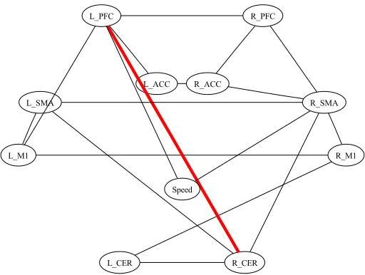
We applied the PCfdr-skeleton and the PC-skeleton algorithms to real-world research tasks,
study-ing the connectivity network between brain regions usstudy-ing functional magnetic resonance imagstudy-ing (fMRI). The purpose of the applications is to check whether the two algorithms correctly curb the error rates in real world applications. The purpose of the applications is not, and also should not be, to answer the question “which algorithm, the PCfdr-skeleton or the PC-skeleton, is superior?”,
for the following reasons. Basically, the two algorithms control different error rates between which there is not a superior relationship (see Appendix C). Secondly, the error rate of interest for a spe-cific application is selected largely not by mathematical superiority, but by researchers’ interest and the scenario of research (see Appendix C). Thirdly, the simulation study has clearly revealed the properties of and the differences (not superiority) between the two algorithms. Lastly, the approx-imating graphical models behind the real fMRI data are unknown, so the comparison on the real fMRI data is rough, rather than rigorous.
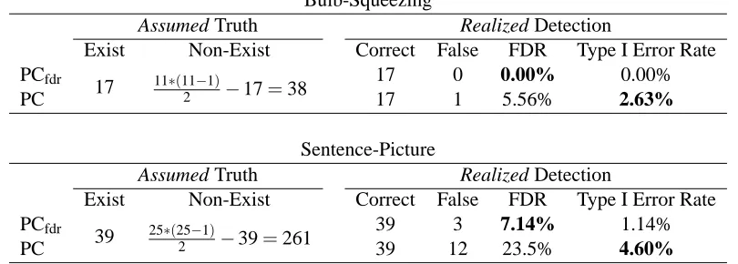
The two algorithms were applied to two real fMRI data sets, one including 11 discrete variables and 1300 observations, and the other including 25 continuous variables and 1098 observations. The first data set, denoted by “the bulb-squeezing data set”, was collected from 10 healthy subjects each of whom was asked to squeeze a rubber bulb with their left hand at three different speeds or at a constant force, as cued by visual instruction. The data involve eleven variables: the speed of squeezing and the activities of the ten brain regions listed in Table 5. The speed of squeezing is coded as a discrete variable with four possible values: the high speed, the medium speed, the low speed, and the constant force. The activities of the brain regions are coded as discrete variables with three possible values: high activation, medium activation and low activation. The data of each subject include 130 time points. The data of the ten subjects are pooled together, so in total there are 1300 time points. For details of the data set, please refer to Li et al. (2008).