Composite Multiclass Losses

Composite Multiclass Losses

Robert C. Williamson

Australian National University and Data61 [email protected] Elodie Vernet

Centre for Mathematical Sciences

University of Cambridge [email protected]

Mark D. Reid

Australian National University and Data61 [email protected]

Editor:Nicolas Vayatis

Abstract

We consider loss functions for multiclass prediction problems. We show when a multiclass loss can be expressed as a “proper composite loss”, which is the composition of a proper loss and a link function. We extend existing results for binary losses to multiclass losses. We subsume results on “classification calibration” by relating it to properness. We determine the stationarity condition, Bregman representation, order-sensitivity, and quasi-convexity of multiclass proper losses. We then characterise the existence and uniqueness of the composite representation for multiclass losses. We show how the composite representation is related to other core properties of a loss: mixability, admissibility and (strong) convexity of multiclass losses which we charac-terise in terms of the Hessian of the Bayes risk. We show that the simple integral representation for binary proper losses can not be extended to multiclass losses but offer concrete guidance re-garding how to design different loss functions. The conclusion drawn from these results is that the proper composite representation is a natural and convenient tool for the design of multiclass loss functions.

Keywords: Proper losses, Multiclass losses, Link Functions, Convexity and quasi-convexity of losses, Margin losses, Classification calibration, Parametrisations and representations of loss functions, Admissibility, Mixability, Minimaxity, Superprediction set

1. Introduction

Machine learning is done for a purpose. The performance of a machine learning solution is judged by means of a loss function. Different choices of loss function will lead to different solutions. The theory of binary losses (i.e. losses suitable for binary prediction problems) is well understood. This paper extends that understanding to multiclass losses and aids the choice of a suitable loss function by exploring the parametrisations available and the implications of different choices. It does so by systematically exploring a decomposition of a multiclass loss into two components, one which affects the statistical performance, and one which affects the computational optimisation of models.

be either predict a label for an unseen instance, or predict the probability that a label takes on a particular value. These two problems are called multiclassclassification andprobability estimationrespectively.

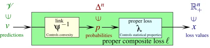
Proper composite lossesare the composition of aproper lossand andinvertible link(both defined formally below). This representation makes the understanding of multiclass losses eas-ier because, crucially, it seperates two distinct concerns: the statistical and the computational. The statistical properties are controlled by the proper loss, while the link function is essentially just a parametrisation. Choice of a suitable link can help—for example, a nonconvex proper loss can be made convex (and thus more amenable to numerical optimisation) by choice of the ap-propriate link. For prediction purposes it is desirable to use anadmissibleloss (one where every possible prediction is uniquely optimal for some underlying distribution). It turns out that every proper composite loss is admissible; in fact proper composite losses satisfy a stronger adequacy property than admissibility.

We characterise when a multiclass loss has a proper composite representation and when such representations are unique. We consider integral representations (whereby the proper component can be expressed as a weighted combination of elementary proper losses). We show the suprising result that there is a fundamental difference betweenn=2 andn>2 in terms of the simplicitly of the parametrisation of the class of elementary proper losses. It has been known for some time that proper losses are characterised by their conditional Bayes risks (or entropy functions). It has already been shown how important properties of a loss that control the performance of certain learning tasks can be expressed directly in terms of the Bayes risk. In this paper we extend results due toReid and Williamson(2010) (forn=2) to generalnand characterise the convexity of a proper loss in terms of the associated Bayes risk.

We also illuminate the connection between classification and probability estimation by char-acterising the relationship between the cruicial property that a loss should have for each of these:

classification calibrated(which we first generalise to make sense in the more general setting we consider) andproperness. We explain the relationship between these two concepts, which cap-tures the idea behind the probing reduction from classification to class probability estimation.

We also show how the results of the paper can provide tools to help with the design of multiclass losses, putting this on firmer ground than in the past.

1.1 Previous Work

With some exceptions, existing work on multiclass loss functions attempts to work directly with `: V →Rn+. As we shall show this conflates two seperate concerns—the design of the

Attribute Previous Work Present Paper Ref.

Structure and Semantics

None—just a function; possibly convex in parameters

Clear seperation of concerns and meaning for λ and ψ. Gives meaning to predictionsvas trans-formed probabilities.

Fig.1

Classification versus probabil-ity estimation

Little insight in the multiclass case; confer recent works such as (Reid and Williamson,2010,

2011;Narasimhan and Agarwal,

2013; Menon and Williamson,

2014) for the binary case

Clear connection via a character-isation relating classification cal-ibrated, prediction calibrated and proper losses

§3

Effect of choice of loss function on performance

Margin based. Only a suffi-cient condition and only for statistical batch setting. Mixes up statistical fundamentals (L) with parametrization (ψ). Strong convexity for speed of convergence in online setting; cf. (Abernethy et al.,2009).

Mixability and Stochastic Mix-ability. Characterisation in on-line setting. Both onon-line worst-case and statistical batch settings. Parametrisation ψ automatically ignored.

§6.1

Admissibility

Not considered explicitly. En-sured however by assuming`is convex.

All proper composite losses ad-missible. All continuous Bayes losses have a proper composite representation.

§6.2

Quasi-convexity and Minimaxity

Guaranteed by assumimg ` is convex.

Quasi-convexity guaranteed for all continuous proper losses; min-imaxity for all continuous proper composite losses.

§6.4

Convexifiability

No principled way to convexify a loss; can make convex surro-gate approximations.

All continuous proper losses con-vexifiable (using the canonical link).

§6.4

Design principles and parametrisa-tion

No guidance; choose` or mar-gin function φ, in which case symmetry imposed.

Principled; general asymmetric losses possible; parametrise via

(Λ,Ψ); separation of concerns.

§8.3

Connections to divergences

Many to one for margin losses in binary case. (Nguyen et al.,

2009)

Explicit 1:1 correspondence for binary and multiclass case (Reid and Williamson, 2011; Garc´ıa-Garc´ıa and Williamson,2012).

§9

Table 1: Comparison of present paper to previous works on loss functions.

2014). Classification calibrated losses are an analog of proper losses for the problem of classifi-cation (Bartlett et al.,2006). The relationship between classification calibration and properness was determined byReid and Williamson(2010) forn=2. Most of these results have had no multiclass analogue until now. Whilst there is much work on classification problems, it is now widely understood that there are often advantages in being able to predict probabilities, rather than just labels (Bennett,2003;Cohen and Goldszmidt,2004).

The theoryof loss functions makes it clear how one ideally chooses a loss—one takes ac-count of one’s utility concerning various incorrect predictions (Kiefer, 1987), (Berger, 1985, Section 2.4). Thepracticerarely involves such a step, primarily, we conjecture, because there is no adequate understanding of the way one can parametrise losses effectively, especially in the multiclass case. There is little guidance in the literature concerning how to choose a loss function; typically heuristic arguments are used for the choice—confer e.g. (Ighodaro et al., 1982;Nayak and Naik,1989). An early approach to multiclass losses is simply reduction to bi-nary (Allwein et al.,2001;Beygelzimer et al.,2007;Crammer and Singer,2001;Dietterich and Bakiri,1995;Zadrozny and Elkan,2002). Related approaches are pairwise coupling or Bradley-Terry models (Hastie and Tibshirani, 1998;Wu and Weng, 2004; Huang et al., 2006) where certain relationships are assumed to hold between the pairwise probabilities and the multivariate probability of interest.

The design of losses for multiclass prediction has received recent attention (Zhang,2004; Hill and Doucet, 2007;Tewari and Bartlett, 2007;Liu, 2007;Santos-Rodr´ıguez et al., 2009; Zou et al.,2008;Zhang et al.,2009) although none of these papers developed the connection to proper losses, and most restrict consideration to margin losses (which imply certain symmetry conditions).Zou et al.(2005) proposed a multiclass generalisation of “admissible losses” (their name for classification calibration) for multiclass margin classification. Liu(2007) considered several multiclass generalisations of hinge loss (suitable for multiclass SVMs) and showed some of them were and others were not Fisher consistent, and when they were not it was shown how the training algorithm could be modified to make the losses behave consistently. Shi et al. (2010) have investigated the relationship between classification calibration of multiclass losses and losses for structure prediction, and have proposed an extension of classification calibration which they call parametric consistency, which attempts to take account of the function class used (classification calibration is, like all the results in this paper, concerned with behaviourper point; in practice one typically optimises over restricted classes of functions). Multiclass losses have also been considered in the development of multiclass boosting (e.g.Zhu et al.,2009;Mukherjee and Schapire,2013;Wu and Lange,2010).

1.2 Outline

The rest of the paper is organised as follows. In§2: we set up the problem formally and state some purely mathematical results we will need;§3: we relate properness, classification calibra-tion, and the notion used byTewari and Bartlett(2007) which we rename “prediction calibrated”;

mixability (§6.1), admissibility (§6.2) and convexity (§6.4), where we give a complete charac-terisation of the (strong) convexity of composite multiclass proper losses in terms of the Bayes risk;§7: we present a (somewhat surprising) negative result concerning the integral representa-tion of proper multiclass losses; §8: we outline how the above results can aid in the design of proper losses, especially by use of a (new) multiclass extension of the “canonical link”; finally,

§9summarises the key contributions and outlines some future directions.

2. Formal Setup

Suppose X is some set andY = [n] ={1, . . . ,n}is a set of labels. (Throughout the papern

is an integer greater than or equal to 2.) We suppose we are given dataS=*(xi,yi)+i∈[m] such thatyi∈Y is the label corresponding toxi∈X. These data follow a joint distributionPX,Y on X ×[n]. We denote by EX,Y andEY|X respectively, the expectation and the conditional

expectation with respect toPX,Y. Given a new observationxwe want to predict the probability

pi:=P(Y =i|X=x)ofxbelonging to classi, fori∈[n]. Multiclass classificationrequires the learner to predict the most likely class ofx; that is to find ˆy∈arg max_i∈[n]pi.

A loss measures the quality of prediction. Let∆n:={(p1, . . . ,pn): ∑i∈[n]pi =1,and 0≤

pi≤1, ∀i∈[n]}denote then-simplex. For multiclass probability estimation,`:∆n→Rn+. The partial losses`i are the components of`(q)= (`1(q), . . . , `n(q))0 and`i(q)is the loss incurred by predictingq∈∆n when y=i. A commonly used loss for probability estimation is thelog

loss `log defined by `log_i (q):=−logqi fori∈[n]. Other examples of multiclass losses we will refer to in this paper include the square loss`sq_i (q):=∑j∈[n](Ji= jK−qj)

2_{, theabsolute loss} `abs<sub>i</sub> (q):=∑j∈[n]|Ji= jK−qj|and the0-1 loss`

01

i (q):=Ji∈arg maxj∈[n]qjK. Here,JPKdenotes the function that is 1 whenPis true and 0 otherwise.

Throughout the paper,A0 denotes transpose of the matrix or vectorA, except when applied to a real-valued function where it denotes derivative. We denote matrix multiplication of com-patible matricesA andB by A·B, so the inner product of two vectors x,y∈Rn isx0·y. The conditional riskLassociated with a loss`is the function

L:∆n×∆n3(p,q)7→L(p,q) =EY∼p`Y(q) =p0·`(q) =

_∑

i∈[n]

pi`i(q)∈R+,

where Y∼ p means Y is drawn according to a multinomial distribution with parameter p∈ ∆n. In a typical learning problem one will construct an estimateq: X →∆n. Thefull riskis

L(q)=EXEY|X`Y(q(X)). Minimizing L(q) overq: X →∆n is equivalent to minimizing L(p(x),q(x))overq(x)∈∆nfor allx∈X wherep(x) = (p1(x), . . . ,pn(x))0, andpi(x) =P(Y=

i|X=x). Thus it suffices to only consider the conditional risk; confer (Reid and Williamson, 2011).

If one is interested in estimating probabilities (`:∆n→Rn+) it is natural to require the asso-ciated conditional risk is minimized when estimating the true underlying probability. Such a loss is calledproper(formally: ifL(p,p)≤L(p,q),∀p,q∈∆n). It isstrictly properif the inequality

is strict when p6=q (so it is uniquely minimised by predicting the correct probability). The conditional Bayes riskis defined by

L:∆n3p7→ inf q∈∆n

V

ψ

∆

v

_p

λ

R

x

`

∈

_∈

_∈

Controls convexity Controls statistical properties link proper loss

proper composite loss

predictions probabilities loss values

ψis a monotone function∆n→V

λis parametrised by a concave Bayes riskΛ:∆n→R

Figure 1: The idea of a proper composite loss.

This function is always concave (Gneiting and Raftery, 2007). If ` is proper, then L(p) = L(p,p) = p0·`(p). Strictly proper losses induceFisher consistentestimators of probabilities: if`is strictly proper, p=arg minqL(p,q). By considering when the derivatives _∂∂qiL(p,q)are

zero it is straight-forward to show that, of the example losses introduced above, the log loss, square loss, and 0-1 loss are proper, while absolute loss is not. Furthermore, both log loss and square loss are strictly proper while 0-1 loss is proper but not strictly proper. Using the fact that, for proper losses, the Bayes riskL(p) =L(p,p)we see thatLlog(p) =−_∑i∈[n]pilogpi(i.e., Shannon entropy);Lsq(p) =1−_∑i∈[n]p_i2; andL01(p) =mini{1−pi}.

The losses above are defined on the simplex∆n since the argument (a predictor) represents

a probability vector. However it is sometimes desirable to use another setV of predictions. For example if one wishes to use linear predictors, their natural range isRn. One can consider losses `:V →Rn+. Suppose there exists an invertible functionψ:∆n→V. Then`can be written as a composition of a lossλ defined on the simplex withψ−1. That is,`(v) =λψ(v):=λ(ψ−1(v)). Such a functionλψ is acomposite loss. Ifλ is proper, we say`is aproper composite loss, with associated proper lossλ andlinkψ; see Figure1. Many commonly used multiclass losses are composite losses, even though they are not often expressed as such; see the example in§8.4.

Throughout the paper,`is a general loss defined onV, whereV may equal∆n, andλ is al-ways a loss defined on∆n, which may be proper. For such a lossλ:∆n→Rn+, its corresponding conditional risk is denotedΛ(p,q)and its conditional Bayes risk isΛ(p).

In order to differentiate the losses we project then-simplex into a subset ofRn−1. Let

˜

∆n:=

(

(p1, . . . ,pn−1)0: pi≥0, ∀i∈[n], n−1

∑

i=1

pi≤1

)

denote the“bottom” of the n-simplex. We denote by

Π∆:∆

n_{3p= (p}

1, . . . ,pn)07→ p˜= (p1, . . . ,pn−1)0∈∆˜n, the projection of the∆n, and

Π−1_∆ : ˜∆n3p˜= (p˜1, . . . ,p˜n−1)07→p= (p˜1, . . . ,p˜n−1,1− n−1

∑

i=1 ˜

pi)0∈∆n

e2

e1

c

T1(c) T2(c)

T3(c)

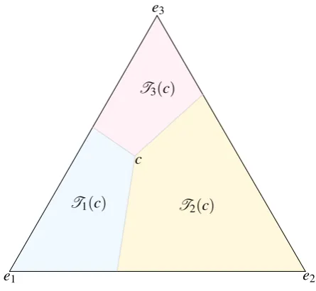
Figure 2: A partitioning of the 3-simplex by regionsTi(c),i=1,2,3, wherec= (.35, .2, .45) as viewed from the direction(1,1,1).

We use the following notation. Thekth unit vectorekis thenvector with all components zero except thekth which is 1. Then-vector1n:= (1, . . . ,1)0. The (relative) interior of the simplex is

˚

∆n:={(p1, . . . ,pn): ∑i∈[n]pi=1,and 0<pi<1,∀i∈[n]}and the boundary is∂∆n:=∆n\∆˚n. We also adopt notation fromMagnus and Neudecker(1999). For the reader’s convenience we list the essential notations and conventions in AppendixA.

3. Relating Properness to Classification Calibration

Properness is an attractive property of a loss for the task of class probability estimation. However if one is merely interested inclassifying(predicting ˆy∈[n]givenx∈X) then it is stronger than one needs. In this section we relate classification calibration (the analog of properness for classification problems) to properness.

Supposec∈_∆˚n_{. We cover}

∆nwithnsubsets each representing one class:

Ti(c):={p∈∆n:∀j6=i picj≥pjci}, i∈[n].

Observe that fori6= j, the setsRi j(c):={p∈∆n: picj=pjci}are subsets of dimensionn−2 throughcand alleksuch thatk6=iandk6= j. These subsets partitionRninto two parts. The set

Ri j(c)is the intersection of∆n and the subspaces delimited by the precedent(n−2)-subspace and in the same side asei. An example of this partition is shown graphically in Figure 2. We will make use of the following properties ofTi(c).

Lemma 1 Suppose c∈_∆˚n_{, i∈[n]. Then the following hold:}

1. For all p∈∆n, there exists i such that p∈Ti(c).

2. Suppose p∈∆n.Ti(c)∩Tj(c)⊆ {p∈∆n: picj=pjci}, a subset of a subspace of

3. Suppose p∈∆n. If p∈T_i=1n Ti(c)then p=c.

4. For all p,q∈∆n, p6=q, there exists c∈∆˚n, and i∈[n]such that p∈Ti(c)and q∈/Ti(c).

The proof is deferred to AppendixB.1.

Classification calibrated losses have been developed and studied under some different def-initions and names (Zhang, 2004; Bartlett et al., 2006). Below we generalise the notion of

c-calibration which was proposed forn=2 by Reid and Williamson(2010) and developed by Scott(2011,2012) as a generalisation of the notion of classification calibration ofBartlett et al. (2006); confer alsoSteinwart(2007).

Definition 2 Suppose`:∆n→Rn+is a loss and c∈∆˚n. We say`isc-calibrated at p∈∆nif for

all i∈[n]such that p∈/ Ti(c) then∀q∈Ti(c), L(p)<L(p,q).We say that`isc-calibratedif

∀p∈∆n,`is c-calibrated at p.

Definition2means that if the probability vectorqone predicts doesn’t belong to the same subset (i.e. doesn’t predict the same class) as the real probability vectorp, then the loss might be larger thanL(p).

Classification calibration in the sense used byBartlett et al.(2006) corresponds to1₂-calibrated losses whenn=2. Ifcmid:= (_n1, . . . ,1_n)0,cmid-calibration induces Fisher-consistent estimates in

the case of classification. Furthermore “`isc<sub>mid</sub>-calibrated and for all i∈[n], and`i is contin-uous and bounded below” is equivalent to “`is infinite sample consistent” as defined byZhang (2004). This is because if`is continuous andTi(c)is closed, then∀q∈Ti(c),L(p)<L(p,q)if and only ifL(p)<infq∈Ti(c)L(p,q).

The following result generalises the correspondence between binary classification calibra-tion and properness (Reid and Williamson,2010, Theorem 16) to multiclass losses (n>2).

Proposition 3 A continuous loss`: ∆n→Rn+ is strictly proper if and only if it is c-calibrated

for all c∈_∆˚n_.

Proof (⇒)Suppose that`is strictly proper. Then for allc∈<sub>∆</sub>˚n<sub>, for alli∈[n]such thatp∈/T</sub> i(c) and for allq∈Ti(c)thenp6=qand thusL(p)<L(p,q)since`is strictly proper.

(⇐)Suppose that`isc-calibrated for allc∈∆˚n. Supposep,q∈∆nandp6=q. By Lemma1

(part4) one can partition pandqinto two different classes: there existsc∈_∆˚n_{andi∈[n]such} thatq∈Ti(c)andp∈/Ti(c). HenceL(p)<L(p,q)since`isc-calibrated. Since`is continuous and∆nis closed, the infimum in the definition ofL(p)is attained. SinceL(p)<L(p,q)for all q6=p, we concludeL(p) =L(p,p). Thus`is strictly proper.

In particular, a continuous strictly proper loss isc_mid-calibrated. Thus for any estimator ˆqn of the conditional probability vector one constructs by minimizing the empirical average of a continuous strictly proper loss, one can build an estimator of the label (corresponding to the largest probability of ˆqn) which is Fisher consistent for the problem of classification.

In the binary case,`is classification calibrated if and only if the following implication holds (Bartlett et al.,2006):

L(fn)→min g L(g)

⇒

PX,Y(Y6= fn(X))→min

g PX,Y(Y6=g(X))

Tewari and Bartlett(2007) have characterised when (1) holds in the multiclass case. Since there is no reason to assume the equivalence between classification calibration and (1) still holds for

n>2, we give different names for these two notions. We useclassification calibrationfor the notion (Definition2) linked to Fisher consistency and useprediction calibrated(defined below) for the notion of Tewari and Bartlett (equivalent to (1)).

Definition 4 Suppose `: V →_Rn

+ is a loss. Let C`:=co({`(v): v∈V}), the convex hull of the image of V. ` is said to be prediction calibrated if there exists a prediction function

pred : Rn→[n]such that

∀p∈∆n: inf

z∈C`:ppred(z)<maxi∈[n]pi

p0·z> inf z∈C`p

0_·

z=L(p).

Suppose that `:∆n→Rn+ is such that ` is prediction calibrated and pred(`(p))∈arg maxipi. Then`isc_mid-calibrated almost everywhere.

By introducing areference linkψ¯ (which corresponds to the actual linkψ if`is a proper composite loss`=λ◦ψ−1) we now show how the pred function can be canonically expressed in terms of arg max_ipi.

Proposition 5 Suppose`:V →R+n is a loss. Letψ¯:∆n→V satisfyψ¯(p)∈arg minv∈<sub>V</sub> L(p,v) andλ=`◦ψ¯. Thenλ is proper. If`is prediction calibrated thenpred(λ(p))∈arg maxi∈[n]pi.

Proof We show first thatλ is proper. Letp∈∆n. Then

Λ(p,p) =L(p,ψ¯(p)) =L(p,arg min v

L(p,v)) =min

v L(p,v)≤qmin∈∆n

Λ(p,q).

Thusλ is proper andL(p) =Λ(p). We now assume that`is prediction calibrated. Suppose that pred(z=λ(p))∈/arg maxipi. Then ppred(λ(p))<maxipi , thus p

0_{·z=Λ(p,p)>L(p) =Λ(p)}

which contradicts the properness ofλ.

4. Characterizing Properness

We now present some simple (but new) consequences of properness in the multiclass case (Proposition6). We also build some connections between the properness of multiclass losses and the properness of binary losses that can be derived from them via a restriction of the multi-class loss to a line connecting two points in then-simplex (Proposition7). Finally, we show that multiclass proper losses are effectively characterised by their Bayes risks (Proposition8) and the continuity of losses is intimately tied to the differentiability of their Bayes risks (Proposition9). An important implication of these last results is that we are able to study the class of multiclass proper losses by focusing our attention on concave functions defined over probabilities.

To state our propositions we need to introduce monotone functions, directional derivatives, and superdifferentials (cf. (Hiriart-Urruty and Lemar´echal,2001)). We say f:C⊂Rn→Rnis monotone(resp.strictly monotone) onCwhen for allxandyinC,

confer (Hiriart-Urruty and Lemar´echal, 2001; Rockafellar and Wets, 2004). If a function f :

Rn→Ris concave then limt↓0

f(x+td)−f(x)

t exists, and is called thedirectional derivativeof fatx in the directiondand is denotedDf(x,d). By analogy with the usual definition ofsubdifferential for convex functions, we introduce thesuperdifferential∂f(x)for concave f atxis

∂f(x):=s∈Rn:s0·y≥Df(x,y),∀y∈Rn

=s∈Rn: f(y)≤f(x) +s0·(y−x),∀y∈Rn .

Similarly, a vectors∈∂f(x)is called asupergradientof f atx.

Proposition 6 Suppose`:∆n→R+n is a loss. If`is proper, then−`is monotone on∆n.

Fur-thermore, if`is strictly proper then it is also invertible.

Proof For all p,q∈∆n,(`(p)−`(q))0·(p−q) = p0·`(p)−q0·`(p) +q0·`(q)−p0·`(q)≤0 sincep0·`(p)≤p0·`(q). For the strictly proper case, we just have to check that`is injective. By way of contradiction assume`is not invertible. Then there exists p6=qsuch that`(p) =`(q). which meansL(p,p) =L(p,q), contradicting the supposed strict properness of`.

The following proposition presents several characterisations of multiclass properness. It shows how the characterisation of properness in the general (not necessarily differentiable) mul-ticlass case can be reduced to the binary case. We also show this is equivalent to testing the properness condition for the loss on all possible line segments joining two distributions within the simplex. This latter characterisation can be viewed as a statement connecting “order sensi-tivity” and properness: the true class probability minimizes the risk and if the prediction moves away from the true class probability in a line then the risk increases. This property appears con-venient for optimisation purposes: if one reaches a local minimum in the second argument of the risk and the loss is strictly proper then it is a global minimum. If the loss is proper, such a local minimum is a global minimum or a constant in an open set. But observe that typically one is minimising the full riskL(q(·))over functionsq:X →∆n. We note that order sensitivity of `doesnotimply this optimisation problem is well behaved; one needs convexity ofq7→L(p,q)

for allp∈∆nto ensure convexity of the functional optimisation problem; we characterise when

that holds in section6.4.

Proposition 7 Suppose`:∆n→Rn+is a loss. We define the binary loss

˜

`p,q:[0,1]3η7→

_˜

`<sub>1</sub>p,q(η) ˜ `₋p,₁q(η)

=

q0·` p+η(q−p) p0·` p+η(q−p)

.

The following statements are equivalent:

1. `is proper;

2. `˜p,q_{is proper for all p,q∈} ∂∆n;

4. there exists a concave function f :∆n→ R and ∀q∈∆n, there exists a supergradient A(q)∈∂f(q)such that∀p,q∈∆n, p0·`(q) =L(p,q) = f(q) + (p−q)0·A(q).

The proof is deferred to AppendixB.3.

Characterisation (2) shows that in order to check if a loss is proper one need only check the properness in each line. One could use the easy characterization of properness for differentiable binary losses (`:[0,1]→_R2

+is proper if and only if∀η∈[0,1],

−`0

1(η)

1−η =

`0−1(η)

η ≥0, (Reid and

Williamson,2010)). However this needs to be checked for all lines defined by p,q∈∂∆n. The above result can also been seen as a generalisation of a result by Lambert(2010) who proved that properness is equivalent to the fact that the further your prediction is from reality, the larger the loss (hence the name “order sensitivity”); also confer the results on monotonicity due toNau (1985). His result relied upon on the total order ofR. In the multiclass case, there does not exist such a total order. Yet, as the above result shows, one can compare two predictions if they are in the same line as the true real class probability.

Characterisation (4) is a restatement of the well known Bregman representation of proper losses; Cid-Sueiro and Figueiras-Vidal (2001) presented the differentiable case, and Gneiting and Raftery(2007, Theorem 3.2) the general case. This last property gives us the form of the proper losses associated with a given Bayes risk. SupposeL:∆n→R+is concave. The proper losses whose Bayes risk is equal toLare

`:∆n3q7→

L(q) + (ei−q)0·A(q)

n

i=1∈R n

+,∀A(q)∈∂L(q). (3)

This result suggests that some information is lost by representing a proper loss via its Bayes risk (when the last is not differentiable). The next proposition elucidates this by showing that proper losses which have the same Bayes risk are equal almost everywhere.

Proposition 8 Two proper losses`1, `2:∆n→Rn+have the same conditional Bayes risk function

L if and only if`1=`2almost everywhere. If L is differentiable,`1=`2everywhere.

Proof A concave function is differentiable almost everywhere (Hiriart-Urruty and Lemar´echal, 2001, theorem 4.2.3). Thus (3) proves that two proper losses `1 and`2 which have the same Bayes risk are equal almost everywhere. Suppose now that two proper losses are equal almost everywhere. Then their associated Bayes risksL1andL2are equal almost everywhere and con-tinuous (since they are concave). If there exists psuch thatL1(p)6=L2(p), then since L1 and

L2are continuous, there existsε >0 such that∀q∈B(p,ε)∩∆n,L1(q)6=L2(q), whereB(p,ε) is a ball of radiusε centred at p. Yet this contradicts the fact thatL1 andL2 are equal almost everywhere. Hence the Bayes risks are equal everywhere.

While the previous proposition shows that losses are closely related to their Bayes risks the next proposition also shows how the continuity of a loss is related to the differentiability of its Bayes risk.

Proposition 9 Suppose`:∆n→Rn+is a proper loss. Then`is continuous in∆˚nif and only if L

is differentiable on∆˚n;`is continuous at p∈_∆˚n_{if and only if L is differentiable at p∈ ˚}

The proof of this result can be found in Appendix B.2. This type of relationship is further explored in Section6.4 where the convexity of a composite loss is related to properties of its Bayes risk.

5. The Proper Composite Representation: Uniqueness and Existence

Many natural predictors have a range other than the simplex (for example those induced by linear functions). It is thus sometimes convenient to define a loss on some setV rather than∆n; confer

(Reid and Williamson,2010). The link function explicates the result ofGr¨unwald and Dawid (2004) that every decision problem induces a decision problem expressed in terms of proper losses; (seevan Erven et al.,2011, section 6, for further explanation).

Traditionally (McCullagh and Nelder, 1989) links are defined only for binary problems (where one is using univariate probabilities). However there is scattered (but seemingly un-systematic) work on multivariate links (Glonek and McCullagh,1995;Glonek,1996), primarily from the perspective of probabilistic modelling (as opposed to the design of loss functions). Sometimes multivariate links are constructed from univariate links (Molenberghs and Lesaffre, 1999).

Composite losses (see the definition in§2) are a way of constructing losses on sets other than

∆n: given a proper lossλ: ∆n→Rn+ and an invertible linkψ:∆n→V, one definesλψ:V →

Rn+ asλψ :=λ◦ψ−1. We now consider the question: given a loss`: V →Rn+, when does` have aproper composite representation(whereby`can be written as`=λ◦ψ−1), and is this representation unique? We first consider the binary case. Here the prediction spaceV ⊆_Ris assumed to be either an interval or the entire real line.

5.1 The Binary Case

Our first result shows that if you can write a binary loss as a proper composite loss, the proper loss defined on the simplex is unique. Furthermore, as soon as the loss is not constant the link function is also unique. If the loss is constant on an interval, then you can choose any value of the link function on this interval which keeps the link function continuous and invertible and still obtain a composite proper loss. The proof can be found in AppendixB.4. As is common in the literature, we write the binary labels as{−1,+1}and so the partial losses are`−1and`+1. Proposition 10 Suppose`=λ◦ψ−1:V →R2+is a proper composite loss and that the proper

lossλ is differentiable and the link functionψ is differentiable and invertible. Then the proper lossλ is unique. Furthermoreψ is unique if ∀v1,v2∈V,∃v∈[v1,v2],`01(v)6=0or`0−1(v)6=0.

If there existsv¯1,v¯2∈V such that`01(v) =`0−1(v) =0∀v∈[v¯1,v¯2], one can choose any ψ|_[v¯1,v¯2] such thatψis differentiable, invertible and continuous in[v¯1,v¯2]and obtain`=λ◦ψ−1, andψ is uniquely defined where`is invertible.

We now determine necessary and sufficient conditions for a binary loss to be expressed as a proper composite loss. Once again, the proof is deferred to SectionB.5.

Proposition 11 Suppose`:V →R2+is a differentiable binary loss such that∀v∈V,`0−1(v)6=0

1. `1is decreasing (increasing);

2. `−1is increasing (decreasing); and

3. f:V 3v7→ `01(v)

`0−1(v)

is strictly increasing (decreasing) and continuous.

Observe that the last condition is alway satisfied if both`1and`−1are convex. 5.2 Binary Margin Losses

Supposeϕ: R→R+ is a function. The loss`ϕ:V 3v7→(`−1(v), `1(v))0= (ϕ(−v),ϕ(v))0∈ R2+ is called a binarymargin loss. Binary margin losses are often used for classification prob-lems. We will now show how the previous proposition applies to them.

Corollary 12 Supposeϕ:R→R+is differentiable and∀v∈R,ϕ0(v)6=0orϕ0(−v)6=0. Then

`ϕ can be expressed as a proper composite loss if and only if f: R3v7→ − ϕ0(v)

ϕ0(−v) is strictly

monotonic continuous andϕis monotonic.

Ifϕ is convex or concave then f defined above is monotonic. However not all binary margin losses are composite proper losses. One can even build a smooth margin loss which cannot be expressed as a proper composite loss. Considerϕ(x) = 1−arctan(x_π −1). Then f(v) = ϕ

0_(v)

ϕ0(−v)= x2+2x+2

x2_−2x+2 which is not invertible. This loss is illustrated in Figure5, after some additional concepts

are introduced.

5.3 The Multiclass Case

Uniqueness of the composite representation remains straightfoward in the multiclass case.

Proposition 13 Suppose a loss `: V → _Rn

+ has two proper composite representations `= λ◦ψ−1 =µ◦φ−1 where λ and µ are proper losses with corresponding Bayes risks Λ and M respectively, andψ andφ are continuous invertible link functions. Thenλ =µ almost every-where.

If`is continuous and has a composite representation, then the proper loss (in the decompo-sition) is unique (λ =µeverywhere).

If`is invertible and has a composite representation, then the representation is unique.

Proof Λ(p) =infqp0·λ(q) =infqp0·`(ψ(q)) =infvL(p,v)(sinceψ is invertible)

=infvL(p,v) =infvL(p,φ(q)) =M(p).

Thenλ andµ are two proper losses which have the same Bayes risk, so these two losses are equal almost everywhere.

∆

-smooth

∀

x

∈

`

(

V

)

∃

!

p

∈

∆

∆

n

-strictly

con

v

ex

∀

p

∈

∆

n

∃

!

x

∈

`

(

V

)

No

Yes

Figure 3: Illustration of∆n-smoothness and ∆n-strict convexity. The hyperplanes witness the

possession or non-possession of the respective properrties.

Characterising the existence of a composite representation is more complex in the multiclass case. We need to introduce some definitions: We make use of a set ofhyperplanesfor p∈∆n

andβ ∈R,

hβ

p:={x∈R n

:x0·p=β}.

A hyperplanehβp supports a setAatx∈Awhenx∈hβp and for alla∈A,a0·p≥β or for all

a∈A,a0·p≤β. Given a loss`:V →Rn+, theloss image`(V):={`(v):v∈V}.

Definition 14 LetS(p,x):=“`(V)is supported by hβp at x for someβ ∈R.”.

1. A loss image`(V)is∆n-strictly convexif for all p∈∆n there exists a unique x∈`(V) such thatS(p,x).

2. A loss image`(V)is∆n-smoothif for all x∈`(V)there exists a unique p∈∆nsuch that S(p,x).

This definition is illustrated in Figure 3. Dropping the uniqueness requirement in these defi-nitions would drastically change things: since we will require`is continuous, `(V) is always closed. Since by assumption`(V)⊂[0,∞)n everysuch loss satisfies the weakened version of

∆n-strict convexity: for all p∈∆n there existsx∈`(V)such thatS(p,x). The weakened

`

(

v

)

`

(

v

)

q

hL₍ q₎ q

=

{_x :_x

·_q

=

L₍ q₎

}

S`

x

=

`

(

v

)

`

(

V

)

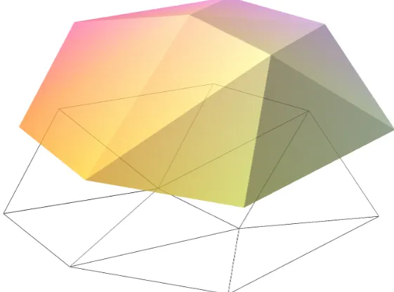
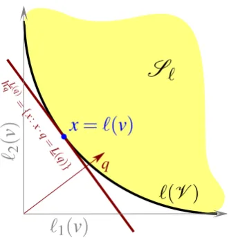
Figure 4: Illustration of geometry of loss functions. The locus of the vector valued loss `is plotted asv varies overV. The superprediction set S` is the region to the “north-east” of the loss image`(V). The hyperplane hL(q)q has normal vector qand offset

L(q). It supportsS`at the pointx=`(v)indicating the Bayes risk is achieved atvfor the true probabilityq.

a convexity-like requirement. (Confer the following result (Schneider, 1993, Theorem 1.3.3):

Suppose A is closed set such thatA˚6=_∅and through each boundary point of A there is a support plane to A; then A is convex.)

The name “∆n-strictly convex” is justified by the observation that replacing∆nbyBln

1 (thel

n 1 unit ball) gives a natural definition of strict convexity of a general set inRn. We also observe that both∆n-strict convexity and∆n-smoothness are closely related to the curvature of the Bayes risk Lby way of the fact that the support function of the set`(V)(restricted to∆n) is the Bayes risk;

confer (Williamson,2014). Specifically,∆n-strict convexity is equivalent to the HessianHL(p)

being non-singular for allp∈∆nwhile∆n-smoothness is implied wheneverL(p)is continuously

differentiable.

SupposeA,B⊂_Rn_{. Then theMinkowski sumA+B:={a+b:a∈A,b∈B}.}

Definition 15 Given a loss`:V →_Rn

+, we denote by

S`:=`(V) + [0,∞)n={x∈Rn+:∃v∈V,∀i∈[n], xi≥`i(v)}

thesuperprediction setof`(Kalnishkan and Vyugin,2008).

One can characterise the existence of proper composite representations in terms of properties the superprediction set. We start with an old result; confer (Dawid,2007).

`1(v) `−

1

(

v

)

S`

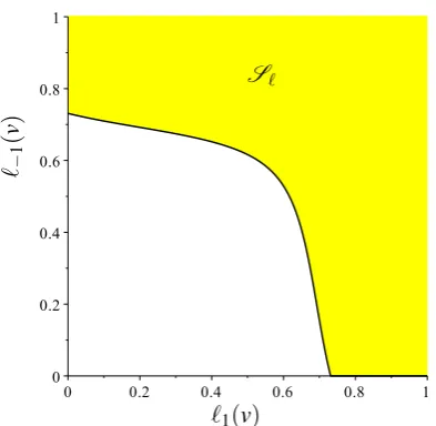
Figure 5: Superprediction set of a binary margin loss which is a not a composite proper loss; See text following Corollary12.

Proof Suppose`is proper butS`is not convex. Then there existsx0∈`(∆n)such that`(∆n)is not supported atx₀ by any hyperplanehpwith normal vector p∈∆n. Letq0∈∆nbe such that `(q0) =x0. Then there is a hyperplanehq0 (with normalq0) that supports`(∆

n_{)at somex} 16=x0. Thusq0₀`(q)is minimised atq1and not minimised atq0and thus`is can not be proper—a con-tradiction.

The geometry of continuous proper losses is illustrated (forn=2) in Figure4. The superpre-diction set of the margin loss discussed following Corollary12isnotconvex as can be seen in Figure5.

Continuous proper losses are quasiconvex, canonically so, as the following result shows.

Proposition 17 Suppose `: ∆n →Rn+ is a continuous proper loss. Then its superprediction

setS` is convex and, for all p∈∆n, the function fp(q):=L(p,q) = p0·`(q)is quasi-convex.

Conversely, suppose fp(q):=p0·`(q)is quasi-convex in q for all p∈∆n. Then there is a unique convex set S such thatT<sub>`</sub>=S and`is necessarily proper.

The proof is in AppendixB.6. Some (but not all) proper losses are in additionconvex; this is studied in more detail in Section6.4below.

Working withS`is problematic for characterising the existence ofstrictlyproper composite representations (essentially because while for a strictly proper loss`,`(∆n)is∆n-strictly convex, S`is not strictly convex (because of the flat spots at the extremes—bounded losses have super-prediction sets with flats parallel to the axes by construction)1. We will thus characterise proper and strictly proper composite representations in terms of properties of`(V)rather thanS`.

Proposition 18 Suppose`:V →Rn+ is a continuous loss. `has a proper composite

represen-tation if and only if`(V)is∆n-smooth. Additionally,`isstrictlyproper composite if and only if

`(V)is also∆n-strictly convex.

The proof is in SectionB.7.

6. Implications: Mixability, Admissibility, Minimaxity and Convexity

We now consider some of the implications that the proper composite representation has for several previously studied properties of loss functions.

6.1 Mixability

Mixability is a fundamental property of a loss function in the study of “prediction with expert advice.” In this setting learning takes place in fixed number of sequential rounds. Each round a learner is presented with predictions some finite number of experts. The learner then makes a prediction and the outcome for that round is revealed. The learner’s and experts’ predictions are assessed using some predefined loss function and the aim of the learner is to incur a total loss not much worse than the best expert –i.e., the one with the smallest total loss. The difference between the learner’s total loss and that of the best expert is known as theregret. In his seminal work,Vovk(1995) showed that no matter how the experts behave, there exists a strategy for the learner (called the “aggregating algorithm”) that guarantees a regret bounded by ln_ηK whereKis the number of experts andηis a positive number called themixability constant(defined below) that only depends on the loss. Losses for which this constant is defined are called mixable. Furthermore, this constantcharacteriseswhen such a constant regret bound is possible. That is, if a loss is not mixable then there is no strategy the learner can use to guarantee a constant regret bound.

Formally, mixability of a loss`is defined in terms of the convexity of a transformation of the loss’s superprediction setS`(see Definition15). We say that forη>0 theη-exponentiated

superprediction set is the image of S` ⊂Rn under the mapping Eη: R

n _→

Rn+ defined by Eη(x):= (e−ηxi)ni=1. A loss `is said to be η-mixable if its η-exponentiated superprediction set is convex. Themixability of`is the smallest value ofηfor which`isη-mixable. For further details, the reader is referred to papers byVovk(1995);Kalnishkan and Vyugin (2008);Vovk and Zhdanov(2009).

Recently,van Erven et al.(2012b)2have shown that the mixability of a loss is related to the curvature of the loss’s Bayes risk relative to the curvature of the Bayes risk for log loss. The main result here builds on some of the insights from that work and shows that mixable losses (under mild conditions) always have proper composite representations.

Forα ∈(0,1)we writeα¯ :=1−α. Forx,y∈Rn,x≤y⇔(xi≤yi, ∀i∈[n]). We now give a necessary condition for mixability.

Lemma 19 Suppose`:V →Rn+, x0=`(v0), x1=`(v1) with x06=x1. Forα ∈(0,1), define x_α:=α¯x0+αx1and vα=α¯v0+αv1. If for someα

xα≤`(vα) (4)

then`is not mixable.

Proof Pick someη >0. Let fη(a) =e−ηa for a∈R so that for x∈Rn we have Eη(x) =

(fη(xi))n_i=1. Observe that the function fη is strictly monotone decreasing (a<b⇒ fη(a)>

f_η(b)) and strictly convex ( ¯αfη(a) +αfη(b)> fη(α¯a+αb)). Fori∈[n]setx0,i=`i(v0)and

x1,i=`i(v1). By assumption, we have ¯

αx0,i+αx1,i≤`i(α¯v0+αv1), ∀i∈[n], which by strict monotonicity

⇒ fη(α¯x0,i+αx1,i)≥fη(`i(α¯v0+αv1)), ∀i∈[n], and hence by strict convexity

⇒α¯ fη(x0,i) +αfη(x1,i)> fη(`i(α¯v0+αv1)), ∀i∈[n]

⇔α¯Eη(`(v0)) +αEη(`(v1))>Eη(`(α¯v0+αv1))

and thus` is not mixable since we have witnessed the non-convexity of the η-exponentiated superprediction set for`.

van Erven et al. (2012b) showed that (under some mild conditions) a proper loss λ and the composite loss λψ obtained via the reference link ¯ψ (see Proposition 5) share the same mixability constant. We now show that mixable losses always have strictly proper composite representations.

Proposition 20 Suppose`:V →Rn+is a∆n-smooth continuous loss. If`is mixable then`has

a strictly proper composite representation.

Proof We prove the contrapositive. Lack of a strictly proper composite representation is equiv-alent then to`(V)being not∆n-strictly convex. Suppose then that`(V)is indeed not∆n-strictly convex. There are two possibilities to consider:

1. There exists p∈∆nsuch that there is nox∈`(V)such that`(V)is supported byhβp atx for someβ ∈R; or

2. There existsp∈∆nsuch that there existsv0,v1∈V,v06=v1,x0=`(v0),x1=`(v1),∃β∈ R, hβp supports`(V)atx1andx2.

6.2 Admissibility

The above results are strongly related to the classical notion of admissibility (Ferguson,1967; Chernoff and Moses,1986;Kiefer,1987), which is particularly simple in our situation. We adapt the terminology ofFerguson(1967) to be consistent with elsewhere in the present paper.

Definition 21 Suppose`:V →_Rn

+is a loss. A prediction v1∈V isbetter thanv2∈V if`(v1)≤ `(v2) and for some i∈[n],`i(v1)< `i(v2). A prediction v1isequivalentto v2 if`(v1) =`(v2).

A prediction v∈V isadmissibleif there is no prediction better than v. If a prediction v∈V is the Bayes-optimal for some distribution p, that is for all v∈V there exists p∈∆nsuch that v∈arg minv_¯∈_V p0·`(v¯), then we say v isstrongly admissible.

Ferguson (1967, Theorem 1, page 60) states the following (which we present for invertible losses, so that`(v<sub>1</sub>) =`(v₂)⇒v₁=v₂).

Proposition 22 Suppose`:V →_Rn

+ is invertible and p∈∆n. If v∈V is the unique prediction

such that L(p,v) =L(p), then v is admissible.

Proposition18then implies the following.

Corollary 23 Suppose`:V →Rn+ is continuous and invertible. If`has a strictly proper

com-posite representation then all v∈V are admissible and strongly admissible.

Proof If`has a strictly proper composite representation, then`(V) is∆n-strictly convex and

thus for all p∈∆n there exists a unique x∈`(V) such thathL(p)p supports `(V) at x. Thus by Proposition 22, v such that`(v) =x is an admissible prediction. Furthermore, since `(V)

is ∆n-smooth, this previous argument actually holds for all v∈V and thus ` is admissible.

Furthermore, it follows directly from the definition of ∆n-smoothness that all v are strongly

admissible.

Proposition 24 If `: V →Rn+ is continuous and has a proper composite representation then

every prediction is admissible.

Proof We will prove the contrapositive: Suppose a continuous loss`:V →_Rn

+is such that there existx0,x1∈`(V)withx1better thanx0. Then`can not have a proper composite representation. Observe that “x1is better thanx0” is equivalent to

∀i∈[n], e0_i·(x₀−x₁)≥0

∃i∈[n], e0_i·(x0−x1)>0. Consider two mutually exclusive and exhaustive cases:

1. e0_i·(x0−x1)>0,∀i∈[n]. Then for allp∈∆n,p0·(x0−x1)>0⇒p0·x0>p0·x1and thus `(V)can not be supported atx<sub>0</sub>byhβp for anyp∈∆nand thus`(V)is not∆n-smooth. 2. Alternatively suppose

e0_i·(x0−x1)

=0, i∈I⊂[n]

>0, i∈[n]\I

(a) pi>0 forsome i∈[n]\I. Thenp0·(x0−x1)>0 and`(V)can not be supported at

x0byhβp for anyβ ∈R.

(b) pi−0 forall i∈[n]\I. Then p0·(x0−x1) =0 in which case`(V)is supported by

hβp for someβ atboth x0andx1.

In either of these subcases, the∆n-smoothness condition is violated.

Thus in both cases we have shown`(V) can not be∆n-smooth and by Proposition18can not have a proper composite representation.

As can be seen in Figure6, there can be no hope of a converse: mere admissibility of every predictionx∈`(V)can not imply that`has a proper composite representation.

However strong admissibility of every prediction implies`(V) is∆n-smooth and so if`is

continuous, strong admissibility of every prediciton implies (via Proposition 18) that ` has a proper composite representation.

The relationship between strict convexity ofS`and admissibility is not new (Brown,1981); but the connection with our characterisation of composite proper losses is new.

We conclude that if ` is continuous and invertible and we desire that all predictions are admissible, then it suffices to only consider losses with a proper composite representation. Con-tinuous invertible losses that do not have a proper composite representation are “redundant” in the sense that there are guaranteed to exist predictions that are not Bayes optimal for any true distribution.

6.3 Minimaxity

We say a loss`:V →Rn+isminimaxif its conditional riskL(p,v) =p0·`(v)satisfies

max p∈∆n

min

v∈_V L(p,v) =minv∈_V maxp∈∆n

L(p,v). (5)

Minimaxity of proper losses has been studied in a very general setting byGr¨unwald and Dawid (2004) who showed the connection between robust Bayes procedures and maximum entropy; confer classical results presented, for example, byFerguson(1967). In this brief subsection we point out some simple implications of our earlier results. Setting V =∆n, oberve that for all

proper lossesλ: ∆n→Rn+, p7→Λ(p,q) =p0·λ(q) is linear for all q∈∆n, and if λ is also continuous, by Proposition17q7→Λ(p,q)is quasi-convex for all p∈∆n. It thus follows from the minimax theorem ofSion(1958) that all continuous proper losses satisfy

max p∈∆n

min q∈∆n

Λ(p,q) =min q∈∆n

max p∈∆n

Λ(p,q) (6)

and are thus minimax.

Suppose `=λψ =λ◦ψ−1: V →Rn+ is a proper composite loss, with conditional risk

L(p,v) =Λ(p,ψ−1(v)). Sinceψ−1is invertible, max

p∈∆n

min

v∈V L(p,v) =maxp∈∆n

min q∈∆n

`

(

v

)

`

(

v

)

hL₍ v) q = {_x :_x ·q = L₍ v₎ }

S

`

x

=

`

(

v

)

`(

V

)

x

=

`

(

v

)

x

=

`

(

v

)

`

(

v

)

`

(

v

)

q

hL₍ v₎ q = {_x :_x ·_q = L₍ v₎ }

S

`

`(

V

)

x

=

`

(

v

)

x

=

`

(

v

)

x

=

`

(

v

)

x

Figure 6: Left:Illustration of a continuous loss`(which can be presumed invertible) with a non-convex superprediction set. For true probabilityq,v1 andv2 both are Bayes optimal sinceq0·`(v₁) =q0·`(v₂) =L(v); thushL(v1)

q =hL(vq 3)supports`(V)at bothx1andx3. The pointx2is never a member of a supporting hyperplane of`(V)and is thus never the Bayes optimal prediction for anyqand so not strongly admissible. The green line indicates the set of predictions that are not strongly admissible—they will never be Bayes optimal forany q∈∆n. Such predictions are, however, admissible, as can be

seen by the grey translated negative orthants centred at x1, x2 andx3 (each orthant does not contain any other predictions “better than” them). All the other predictions whose image lies in the black line are both admissible and strongly admissible. The loss image`(V)is not∆n-smooth because there exist nop∈∆nthat supports`(V)at x2. Hence by Proposition18,`can not have a proper composite representation.Right:

Similar to the figure on the left, except there are now some predictions, such asx₂, which are not admissible: x4isbetter than x2 as can be seen sincex4 is contained in the interior of the shifted negative orthant centred atx2. Note in this case the boundary of the super-prediction setS`does not equal`(V)(see the part ofS`cross-hatched in red). This loss can not have a proper composite representation by Proposition24.

where by the relationship betweenqandv, arg min v∈V

L(p,v) =ψ arg min q∈∆n

Λ(p,q) !

. Similarly,

min v∈_V maxp∈∆n

L(p,v) =min q∈∆n

max p∈∆n

Λ(p,q). (8)

Sinceλ is proper,Λsatisfies (6) which combined with (7) and (8) proves the following.

Proposition 25 Every continuous proper composite loss is minimax.

general inRnbecause convexity preserving mappings must be affine (Webster,1994, Theorem 7.3.7); confer (Meyer and Kay,1973). Recall Proposition17showed the quasi-convexity of all proper losses.

Proposition 25 means that the use of the classical minimax theorem by Abernethy et al. (2009) in order to prove their main result forconvex losses can be foregone; their result also holds for arbitrary continuous proper composite losses.

6.4 Convexity

In order to computationally optimise models with respect to a loss function it is convenient if the loss is convex. In this subsection we develop conditions for the convexity of multiclass composite proper losses. We assume throughout this section that the loss and link are twice differentiable. We start by proving some identities for their first and second derivatives.

6.4.1 TECHNICALPRELIMINARIES

Suppose`=λ◦ψ−1 is composed of the proper lossλ: ∆n→Rn+ and the inverse of the link ψ: ∆n→V. In order to simplify the calculation of derivatives for the function `: V →Rn+ we will assume the setV is a flat,(n−1)-dimensional, convex subset ofRn+. We do so since if V were some arbitrary manifold the extra definitions required to make sense of convexity (e.g., in terms of geodesics) and derivatives on manifolds would obscure the gist of the results below. Furthermore, little is lost either practically or theoretically by assuming a simple V. In practice, predictions are usually vectors in Rn+, and in theory one could always choose a parametrisation ofV in terms of some simpler spaceU and redefine the link via composition with that parametrisation. Alternatively, since links must be invertible, a composite loss could be defined by a choice of loss and choice ofinverse linkψ−1:V →∆nfor aV assumed to be

flat,etc.

Recalling the convention that ˜n:=n−1, letv∈V fixed but arbitrary with corresponding ˜

p=ψ˜−1(v)whereψ˜(p˜):=ψ((p˜1, . . . ,p˜n,˜ pn)0)with pn:=∑ni=1˜ p˜iis the induced function from ˜

∆n to V. By the chain rule and the inverse function theorem, the derivatives for each of the

partial losses`isatisfy

D`i(v) =Dλi(ψ˜−1(v))=Dλi(p˜)·[Dψ˜(p˜)]−1. (9) We use en_i to denote the ith n-dimensional unit vector, en_i = (0, . . . ,0,1,0, . . . ,0)0 when

i∈[n], and define en_i =0n when i>n. We can now write Dλi(p˜) in terms of the n×n˜ ma-trixDλ(p˜) using Dλi(p˜) = (eni)0·Dλ(p˜). Now Dλ(p˜) = (Dλ˜(p˜)0,Dλn(p˜)0)0, where ˜λ(p˜) =

(λ1(p˜), . . . ,λn˜(p˜))0, and so

Dλi(p˜) = (eni)0·Dλ(p˜) = (eni)0·

Dλ˜(p˜)

Dλn(p˜)

. (10)

Furthermore, since λ is proper, Lemma 6 of (van Erven et al.,2012b) means we can use the relationship between a proper loss and its projected Bayes riskL˜ :=L◦Π−_∆1to write

Dλ˜(p˜) =W(p˜)·HL˜(p˜) (11)

whereW(p˜):=In˜−1n˜·p˜0and wherey(p˜):=−p˜/pn(p˜)andpn(p˜):=1−∑i∈[n]˜ pi. Thus, combining (10–12) we have for alli∈[n˜]

Dλi(p˜) = (eni˜)0·W(p˜)·HL˜(p˜)

= ((en_i˜)0−(en_i˜)0·1n_˜·p˜0)·HL˜(p˜)

= (en_i˜−p˜)0·HL˜(p˜) (13)

and

Dλn(p˜) =y(p˜)0·W(p˜)·HL˜(p˜)

= −1

pn(p˜) ˜

p0·(In˜−1n˜·p˜0)·HL˜(p˜)

= −1

pn(p˜)

(p˜0−(1−pn(p˜))p˜0)·HL˜(p˜)

=−p˜0·HL˜(p˜). (14)

Finally, noting that by definitionen˜

n=0, (14) and (13) can be merged and combined with (9) to obtain the following proposition.

Proposition 26 For all i∈[n],p˜∈∆˚˜n(the relative interior of∆˜n), and v=ψ˜(p˜),

D`i(v) =− en_i˜−p˜0·κ(p˜) (15) where

κ(p˜):=−HL˜(p˜)·[Dψ˜(p˜)]−1. (16) Using the definition of the HessianH`i=D[(D`i)0]and the product rule (31) gives

D(D`i(v))0=Dv[

f(p)˜

z }| {

Dψ˜(p˜)0−1·HL˜(p˜)0· g(p)˜

z }| {

en_i˜−p˜] =

en_i˜−p˜0⊗In˜

·Dv[f(p˜)0+ (I1⊗f(p˜))·D eni˜−ψ˜

−1_(v) = en_i˜−p˜0⊗In˜

·DvhHL˜(p˜)·[Dψ˜(p˜)]−1i−

Dψ˜(p˜)0−1

HL˜(p˜)0·[Dψ˜(p˜)]−1, whereDv is used to indicate that the derivative is with respect toveven when the terms inside the derivative are expressed using ˜p. We have now established the following proposition.

Proposition 27 For all i∈[n],p˜∈∆˚˜n, and v=ψ˜(p˜),

H`i(v) =− e_in˜−p˜0⊗In˜

·D

κ ψ˜−1(v)

+ κ(p˜)0

·[Dψ˜(p˜)]−1,

The product κ(p˜):=−HL˜(p˜) [Dψ˜(p˜)]−1 that appears in both propositions above can be interpreted as the curvature of the Bayes risk function ˜Lrelative to the rate of change of the link function ˜ψ. When the link function is the identity ˜ψ(p˜) = p˜ (i.e.when we have a proper loss directly) the expressions for the derivative and Hessian of each`isimplify to

D`i(p˜) = (en_i˜−p˜)0·HL˜(p˜) (17)

H`i(p˜) = e_in˜−p˜0⊗In˜

·D

HL˜(p˜)

−HL˜(p˜)0. (18)

The form ofκ as the product ofHL˜ andDψ˜ suggests another simplification.

Definition 28 Thecanonical link functionfor a lossλ with Bayes risk L is defined via

˜

ψ_λ(p˜):=−DL˜(p˜)0. (19)

We will show in section8.1 that (19) is indeed guaranteed to be a legitimate link. The termκ simplifies toκ(p˜) =In˜sinceDψ˜(p˜) =−D(DL˜(p˜)0) =−HL˜(p˜). For this choice of link function, the first and second derivatives become considerably simpler.

Proposition 29 Ifλ:∆n→Rn+is a proper loss andψ˜λis its associated canonical link then, for

all i∈[n],p˜∈∆˚˜n, and v=ψ˜λ(p˜), the composite loss`=λ◦ψ˜ satisfies

D`i(v) = (en_i˜−p˜) (20)

H`i(v) =HL˜(p˜)−1. (21) The simplified form of the Hessian above is established by noting that sinceκ(p˜) =In˜we have D[κ(ψ˜−1(v))] =0 for allv∈V in Proposition27.

The above propositions hold for any number of classes n. It is instructive (both here and later in the paper) to examine the binary case wheren=2. In this case, Proposition 26 and Proposition27reduce to

`0<sub>1</sub>(v) =−(1−p˜)κ(p˜) ; `0₂(v) =p˜κ(p˜) (22) `00₁(v) = −(1−p˜)κ

0_{(p˜) +} κ(p˜) ˜

ψ0(p˜) (23)

`00₂(v) = p˜κ 0_{(p˜) +}

κ(p˜) ˜

ψ0(p˜) (24)

whereκ(p˜) =−L˜ 00

(p)˜ ˜

ψ0(p)˜ ≥0 and so d dvκ(ψ˜

−1_{(v)) =} κ0(p)˜ ˜

ψ0(p)˜ .

6.4.2 CONDITIONS FOR CONVEXITY OF MULTICLASS COMPOSITE PROPER LOSSES

even in the binary case because here we consider strongly convex losses. We will also show how any non-convex proper loss can be made convex by suitable choice of a link function (the canonical link)3.

For a convex setC⊆Rn, a loss`:C→Rn+ is said to be convexif for all p∈∆n, the map

C3v7→L(p,v) =p0·`(v)is convex. That is, a loss is convex if, under any distribution pover outcomesi∈[n], the expected lossEi∼p[`i(v)]is convex inv. It is easy to see that`is convex if and only if`i:C→R+is convex for alli∈[n]. (The “if” part follows since a sum of convex functions is convex; the “only if” follows by considering p=ei, fori∈[n].)

Definition 30 Suppose C⊆Rn is convex. A function f:C→Risstrongly convex onCwith

modulusc≥0if for all x,x₀∈C,∀α ∈(0,1),

f(αx+ (1−α)x0)≤αf(x) + (1−α)f(x0)− 1

2cα(1−α)kx−x0k 2_.

Whenc=0 in the above definition, f is convex. The function f is strongly convex onCwith moduluscif and only ifx7→ f(x)−c

2kxk

2_{is convex onC(Hiriart-Urruty and Lemar´echal,2001,} page 73). Therefore, the mapsv7→`i(v)arec-strongly convex if and only ifH`i(v)<cIn. By˜ applying Proposition 27we obtain the following characterisation of the c-strong convexity of the loss`.

Proposition 31 A proper composite loss`=λ◦ψ−1is strongly convex with modulus c≥0if and only if for allp˜∈∆˚˜nand for all i∈[n]

en_i˜−p˜ ⊗In_˜

·D κ ψ˜−1(v)4κ(p˜)0·[Dψ˜(p˜)]−1−cIn.˜ (25) We now consider the implications of Proposition31in two special cases: in the multiclass case with canonical link, and in the binary case with the identity link.

Recall that the canonical link ˜ψ`is chosen so that ˜ψ(p˜) =−DL˜(p˜)0. This simplifiesκ(p˜)to the identity matrixIn˜ soDκ(p˜) =0. In this case the above proposition reduces to the following corollary.

Corollary 32 If`=λ◦ψ−1is defined so thatψ˜ =−DL˜0then each map v7→`i(v)is c-strongly convex if and only if−HL˜(p˜)−1

<cIn˜, or equivalently−HL˜(p˜)41_cIn˜.

An immediate consequence of this result is obtained by observing that the definiteness constraint is always met when c=0 since ˜Lis always a concave function. Thus, using a canonical link guarantees a proper composite loss is convex.

There is an upper definiteness condition analogous to that for strong convexity that has im-plications for rates of convergence in numerical optimisation. Boyd and Vandenberghe(2004,

§9.1.2) show that if a twice differentiable function f:X →_Rsatisfies

MI_<Hf(x)<mI

for allx∈X ⊂Rnthen the value M_m is an upper bound on thecondition numberofHf, that is, the ratio of maximum to minimum eigenvalue ofHf. This value measures the eccentricity of the sublevel sets of f and controls the rate at which optima of f are approached.

Applying this result to the Hessian of a composite loss`with a canonical link shows that the condition number bound is controlled by the Hessian of the Bayes risk of`. Specifically, if the condition number is to be no more thanM/mthen _M1 <−HL˜(p˜)<m1 for all ˜p. In the case thatM=mand the condition number is 1, the only Hessian that satisfies these conditions is HL˜(p˜) =−In_˜which is easily shown to be the Bayes risk for square loss. Thus, square loss is the only canonical composite loss for which a condition number of 1 is possible.

In the binary case, whenn=2, (23) and (24) and the positivity of ˜ψ0 simplify (25) to the two conditions:

(1−p˜)κ0(p˜) ≤ κ(p˜)−cψ˜0(p˜)

−p˜κ0(p˜) ≤ κ(p˜)−cψ˜0(p˜)

, ∀p˜∈(0,1).

Further assuming that ˜ψis the identity link ( ˜ψ(v) =v) and lettingw(p˜):=−L˜00(p˜)gives

w0(p˜) ≤ 1

1−p˜(w(p˜)−c))

w0(p˜) ≥ −1 ˜

p (w(p˜)−c)

)

, ∀p˜∈(0,1)

⇔ −1

˜

p ≤

w0(p˜) w(p˜)−c ≤

1

1−p˜, ∀p˜∈(0,1). (26)

The last equivalence is achieved by dividing through byw(p˜)−c which must necessarily be positive since if it were not the final pair of inequalities would imply−1

˜ p≥

1

1−p˜, a contradiction given that ˜p∈[0,1]. Note that (26) reduces to (Reid and Williamson,2010, Corollary 26) for

c=0.

Observe that ifg(p˜):=log(w(p˜)−c)theng0(p˜) = _w(w0_p)˜(p)˜_−c is the middle term in (26). This allows a simplification of the inequality. Specifically, if we assumew(1₂) =1 then

−1

˜

p ≤ g

0₍

˜

p) ≤ 1

1−p˜, ∀p˜∈(0,1)

⇒ Z q 1 2 −1 ˜

pdp˜ Q

Z q

1 2

g0(p˜)dp˜ _Q

Z q

1 2

1

1−p˜dp˜,∀q∈(0,1)

⇔ −log(q)−log(2) Q g(q)−log(1−c) (27)

Q −log(2)−log(1−q),∀q∈(0,1)

⇔ 1

2q Q e

g(q)−log(1−c) _Q 1

2(1−q),∀q∈(0,1)

0 0.25 0.5 0.75 1 1

2 3 4

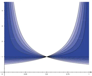
Figure 7: Graph ofw(p˜) =−_L˜00_{(p˜)as a function of ˜pnecessary for a suitably normalised binary} proper loss to be strongly convex with modulusc∈ {0,1₅,2₅,3₅,4₅,1}. The regionsRc are nested by subsethood so thatR₀⊃R_1/5⊃R_2/5⊃R_3/5⊃R_4/5⊃R₁, whereR₁is simply the dotted line (containing only the functionw(c) =1,∀c∈[0,1], which is the weight function corresponding to squared loss). The palest shaded region corresponds toR₀, the allowable range ofw(c)necessary for the corresponding proper loss to be convex, and the darkest corresponds toR₄/5.

Proposition 33 Let w(p˜) =−HL˜(p˜) =−L˜00(p˜)and assume w(1/2) =1. A proper binary loss

`:∆2→R2+is strongly convex with modulus c∈[0,1]only if 1

2 ˜p Q

w(p˜)−c

1−c Q

1

2(1−p˜), ∀p˜∈(0,1), (28)

whereQdenotes≤for p˜≥1

2 and denotes≥for p˜≤ 1 2.

The above proposition only gives a necessary condition for strong convexity. (In addition towbelonging to the specified region,w0(p˜)also needs to be suitably controlled). A sufficient condition is useful for designing strongly convex proper losses. Observe that if

w(p˜) =exp

Z p˜

1/2

u(t)dt+K

+c

whereu:[0,1]→_RandK,c∈_R, then ∂

∂p˜log(w(p˜)−c) =u(p˜). We requirew(1/2) =1 and so exp

R1/2

1/2u(t)dt+K

+c=1 and soeK=1−cand

w(p˜) = (1−c)exp

Z p˜

1/2

u(t)dt

+c (29)

satisfies (26) if

−1

˜

p ≤u(p˜)≤

1

1−p˜, ∀p˜∈(0,1), (30)

and hence the loss with weight functionwis strongly convex with modulusc. Thus by choosing

uto satisfy (30) and constructingwvia (29) one can design strongly convex proper binary losses. One can ask whether equation (25) can be simplified in the n>2 case by using a matrix version of the logarithmic derivative trick in a manner similar to that used above whenn=2. Such a result does exist (Horn and Johnson,1991, Section 6.6.19) but it requires that(HL˜(p˜))−1 andD(HL˜(p˜))commute for all ˜p∈∆˜n, which is not generally the case.

7. Integral Representations of Proper Losses

Binary proper losses have an attractive integral representation that provides substantial insight and is a useful tool for both designing losses and understanding the implications of different choices of loss. Specifically, there exists a family of “extremal” loss functions (cost-weighted generalisations of the 0-1 loss) parametrised by c ∈[0,1] and defined for all η ∈ [0,1] by `c<sub>−1</sub>(η):=c<sub>J</sub>η ≥c<sub>K</sub>and`c₁:= (1−c)_Jη<c_K. As shown byBuja et al. (2005) and Reid and Williamson(2011), given these extremal functions, any proper binary loss`can be expressed as the weighted integral

`=

Z 1

0

`cw(c)dc+constant

with “weight function”w(c) =−_L˜00_{(c). This representation is a special case of a representation} from Choquet theory (Phelps,2001;Simon,2011) which characterises when every point in some set can be expressed as a weighted combination of the “extremal points” of the set. Although there is such a representation when n>2, the difficulty is that the set of extremal points is

much larger and this rules out the existence of a nice small set of “primitive” proper losses whenn>2, and consequently rules out an easy-to-work-with weight function parameterizing all possible multiclass lossses in a manner analogous to the binary case. The rest of this section makes this statement precise.

A convex cone K is a set of points closed under positive linear combinations. That is,