A Cure for Variance Inflation in High Dimensional Kernel Principal
Component Analysis
Trine Julie Abrahamsen [email protected]
Lars Kai Hansen [email protected]
DTU Informatics
Technical University of Denmark
Richard Petersens Plads, 2800 Lyngby, Denmark
Editor: Manfred Opper
Abstract
Small sample high-dimensional principal component analysis (PCA) suffers from variance infla-tion and lack of generalizability. It has earlier been pointed out that a simple leave-one-out vari-ance renormalization scheme can cure the problem. In this paper we generalize the cure in two directions: First, we propose a computationally less intensive approximate leave-one-out estimator, secondly, we show that variance inflation is also present in kernel principal component analysis (kPCA) and we provide a non-parametric renormalization scheme which can quite efficiently re-store generalizability in kPCA. As for PCA our analysis also suggests a simplified approximate expression.
Keywords: PCA, kernel PCA, generalizability, variance renormalization
1. Introduction
While linear dimensionality reduction by principal component analysis (PCA) is a trusted machine learning workhorse, kernel based methods for non-linear dimensionality reduction are only starting to find application. We expect the use of non-linear dimensionality reduction to expand in many applications as recent research has shown that kernel principal component analysis (kPCA) can be expected to work well as a pre-processing device for pattern recognition (Braun et al., 2008). In the following we consider non-linear signal detection by kernel PCA followed by a linear discriminant classifier.
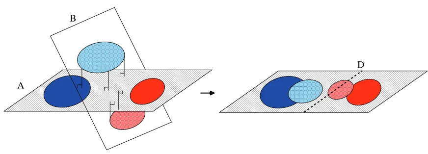
In spite of its conceptual simplicity and ubiquitous use, principal component learning in high dimensions is in fact highly non-trivial (see, e.g., Hoyle and Rattray, 2007; Kjems et al., 2001). In the physics literature much attention has been devoted to learnability phase transitions. In PCA there is a sharp transition as function of sample size from no learning at all to a regime where the projections become more and more accurate. In the transition regime where learning is still incomplete there is a mismatch between the test and training projections. In Kjems et al. (2001) it was shown that this can be interpreted as a case of over-fitting and leads to pronounced variance inflation in the training set projections and results in lack of generalization to test data as illustrated in Figure 1.
0000000000 0000000000 0000000000 0000000000 0000000000 0000000000 0000000000 0000000000
1111111111 1111111111 1111111111 1111111111 1111111111 1111111111 1111111111 1111111111
0000000000000000000000000000000000000000000000000000 0000000000000000000000000000000000000000000000000000 0000000000000000000000000000000000000000000000000000 0000000000000000000000000000000000000000000000000000 0000000000000000000000000000000000000000000000000000 0000000000000000000000000000000000000000000000000000 0000000000000000000000000000000000000000000000000000 0000000000000000000000000000000000000000000000000000 0000000000000000000000000000000000000000000000000000 0000000000000000000000000000000000000000000000000000 0000000000000000000000000000000000000000000000000000 0000000000000000000000000000000000000000000000000000
1111111111111111111111111111111111111111111111111111 1111111111111111111111111111111111111111111111111111 1111111111111111111111111111111111111111111111111111 1111111111111111111111111111111111111111111111111111 1111111111111111111111111111111111111111111111111111 1111111111111111111111111111111111111111111111111111 1111111111111111111111111111111111111111111111111111 1111111111111111111111111111111111111111111111111111 1111111111111111111111111111111111111111111111111111 1111111111111111111111111111111111111111111111111111 1111111111111111111111111111111111111111111111111111 1111111111111111111111111111111111111111111111111111
0000000000000000000000000000000000000000000000000000 0000000000000000000000000000000000000000000000000000 0000000000000000000000000000000000000000000000000000 0000000000000000000000000000000000000000000000000000 0000000000000000000000000000000000000000000000000000 0000000000000000000000000000000000000000000000000000 0000000000000000000000000000000000000000000000000000 0000000000000000000000000000000000000000000000000000 0000000000000000000000000000000000000000000000000000 0000000000000000000000000000000000000000000000000000 0000000000000000000000000000000000000000000000000000
1111111111111111111111111111111111111111111111111111 1111111111111111111111111111111111111111111111111111 1111111111111111111111111111111111111111111111111111 1111111111111111111111111111111111111111111111111111 1111111111111111111111111111111111111111111111111111 1111111111111111111111111111111111111111111111111111 1111111111111111111111111111111111111111111111111111 1111111111111111111111111111111111111111111111111111 1111111111111111111111111111111111111111111111111111 1111111111111111111111111111111111111111111111111111 1111111111111111111111111111111111111111111111111111 00000000000000
00000000000000 00000000000000 00000000000000 00000000000000 00000000000000 00000000000000 00000000000000 00000000000000 00000000000000
11111111111111 11111111111111 11111111111111 11111111111111 11111111111111 11111111111111 11111111111111 11111111111111 11111111111111 11111111111111
00000000 00000000 00000000 00000000 00000000 00000000 00000000
11111111 11111111 11111111 11111111 11111111 11111111 11111111
0000000000 0000000000 0000000000 0000000000 0000000000 0000000000 0000000000 0000000000
1111111111 1111111111 1111111111 1111111111 1111111111 1111111111 1111111111 1111111111
B
A
D
Figure 1: Illustration of the variance inflation problem in PCA. Because PCA maximizes variance, small data sets in high dimensions will be overfitted. When the PCA subspace (A) is applied to a test data set (B) the projected data will have smaller variance. This leads to lack of generalizability if the training data is used to train a classifier, say a linear discriminant (D). In Kjems et al. (2001) this problem was noted and it was shown that the necessary renormalization can be estimated in a leave-one-out procedure
be reduced effectively by a leave-one-out (LOO) scale renormalization of the PCA test projections to restore generalizability (Kjems et al., 2001). In this paper we pursue several extensions of this result. We give a straightforward geometric analysis of the projection problem that suggests a com-putationally less intensive approximate cure than the one originally proposed by Kjems et al. (2001). Next, we proceed to investigate the issue in the context of kernel based unsupervised dimensionality reduction. We show in both simulation and in real world data (USPS handwritten digits and func-tional MRI data) that variance inflation also happens in kPCA and basically for the same reasons as in PCA. We then provide an extension to the LOO procedure for kPCA which can cope with potential non-Gaussian distributions of the kPCA projections, and finally we propose a simplified approximate renormalization scheme.
2. Generalizability in PCA
0 50 100 150 200 250 300 0
0.1 0.2 0.3 0.4 0.5 0.6 0.7 0.8 0.9 1
Overlap with symmetry breaking direction
Training set size (N)
Simulation Theoretical
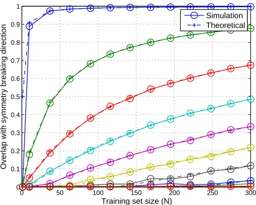
Figure 2: Phase transitions in PCA. Simulated data was created as x=ηu+ǫ, with a nor-mal distributed signal of unit strength η∼N(0,1), embedded in i.i.d. normal noise ǫ∼N(0,σ21). In this simulated data set we show the phase transition like behavior
of the overlap (the mean square of the projection) of the first PCA eigenvector and the signal directionu. The input space has dimension D=1000, and the curves are for 10 values of signal to noise within the intervalσ∈[0.01,0.5]. For a noise level of, for ex-ample, σ=0.17 (black curves) there is a sharp transition both in the theoretical curve (dash/cross) and the experimental curve (full/circle) around N=120 examples.
phase transition depends on the signal variance to noise variance ratio (SNR). The theoretical result provides a mean bias for a specific model, hence, cannot directly be used to restore generalizability in a given data set.
Now, what happens to the generalization performance of PCA in the noisy region? The PCA projections will be offset by different angles depending on how severe the given component is affected by the noise. Because of the bias the test projections will follow different probability laws than the training data, typically with much lower variance. Hence, if we train a classifier on the training projections the classifier will make additional errors on the test set as visualized in Figure 1.
−2 −1 0 1 2 −4
−2 0 2 4
Approximation
PC 1
−1.5 −1 −0.5 0 0.5 1 1.5 2 −2
0 2 4
PC 2
−1 −0.5 0 0.5 1 −2
0 2 4
Approximation
LOO projection PC 3
−0.5 0 0.5 −2
0 2
LOO projection PC 4
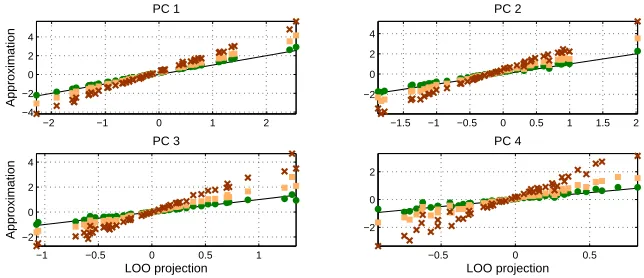
Figure 3: Approximating the leave-one-out (LOO) procedure. Here we simulate data with four normal independent signal components,x=Σ4
k=1ηkuk+ǫof strengths(1.4,1.2,1.0,0.8,
embedded in i.i.d. normal noise ǫ ∼N(0,σ21), with σ=0.2. The dimension was
D=2000 and the sample size was N =50. In the four panels we show the training set projections (red crosses), the projections corrected for the theoretical mean overlap (Hoyle and Rattray, 2007) (yellow squares) and the geometric approximation in Equation (1) (green dots) versus the exact LOO projections (black line).
Let{x1, . . . ,xN}be N training data points in a D dimensional input space
X
(see notation),1weconsider the case N≪D. The LOO step for the N’th pointxN concerns projecting onto the PCA
eigenvectors derived from the subset {x1, . . . ,xN−1}. Define the orthogonal and parallel
compo-nents of the test point,xN=x⊥N+x k
N, relative to the subspace spanned by the training data. As the
PCA eigenvectors with non-zero variance are all in the span of the training data we obtain
uTN−1,k·xN=uTN−1,k·x k N ,
whereuN−1,kis the k’th eigenvector of the LOO training set. Assuming that the changes in the PCA
eigenvectors going from sample size N to N−1 are small, we can approximate the test projections as
uTN−1,k·xN=uTN−1,k·x k
N≈uTN,k·x k
N, (1)
whereuN,k is the k’th eigenvector on the full sample. The approximation introduces a small error
of order 1/N as discussed in detail in the Appendix and further illustrated in a simulation data set in Figure 3. Note that the orthogonal projectionsxkN of the N points may be calculated from the inverse matrix of the inner products of all data points, in N steps each of a cost scaling as N2, thereby achieving a computational burden which scales as N3rather than the N4 scaling for an exact LOO procedure proposed in Kjems et al. (2001).
3. Renormalization Cure for Variance Inflation in kernel PCA
The statistical properties of kernel PCA have also been studied extensively by Blanchard et al. (2007), Hoyle and Rattray (2004a), Hoyle and Rattray (2004b), Mosci et al. (2007), Shawe-Taylor and Williams (2003) and Zwald and Blanchard (2006), but to our knowledge the geometry of gen-eralization for kPCA has not been discussed in the extremely ill-posed case N≪D.
To better understand the variance inflation problem in relation to kPCA let us recapitulate some basic aspects of this non-linear dimensional reduction technique.
Let
F
be the Reproducing Kernel Hilbert Space (RKHS) associated with the kernel function k(x,x′) =ϕ(x)Tϕ(x′), whereϕ :X
7→F
is a possibly non-linear map from the D-dimensionalinput space
X
to the high dimensional (possibly infinite) feature spaceF
. In kPCA the PCA step is carried out in the feature space,F
, mapped data (Sch¨olkopf et al., 1998). However, asF
can be infinite dimensional we first apply the kernel trick allowing us to work with the Gram matrix of inner products. Let{x1, . . . ,xN}be N training data points inX
and{ϕ(x1), . . . ,ϕ(xN)}be thecorresponding images in
F
. The mean of theϕ-mapped data points is denoted ¯ϕand the ‘centered’ images are given by ˜ϕ(x) =ϕ(x)−ϕ¯. The kPCA is performed by solving the eigenvalue problem fKαi=λiαiwhere the centered kernel matrix,Kf, is defined as
f
K=K− 1
N1NNK− 1
NK1NN+ 1
N21NNK1NN. (2)
The projection of aϕ-mapped test point onto the i’th component is given by
βi=ϕ˜(x)Tvi= N
∑
n=1αinϕ˜(x)Tϕ˜(xn) = N
∑
n=1αin˜k(x,xn), (3)
wherevi is the i’th eigenvector of the feature space covariance matrix and theαi’s have been
nor-malized. The centered kernel function can be found as ˜k(x,x′) =k(x,x′)−1
N11Nkx−
1
N11Nkx′+
1
N211NK1N1, wherekx= [k(x,x1), . . . ,k(x,xN)]T. The projection ofϕ(x)onto the first q
princi-pal components will in be denoted Pq(x).
In the following we focus on a Gaussian kernel of the form k(x,x′) =exp(−1c||x−x′||2), where
c is the scale parameter controlling the non-linearity of the kernel map. By the centering operation, PCA is the obtained in the limit when c→∞. Thus for large values we expect variance inflation to be present due the reasons discussed above. What happens in the non-linear regime with a finite c? To answer this question we analyze the LOO scenario for kPCA.
Consider the squared distance ||xn−xN||2 in the exponent in the Gaussian kernel for some
training set pointxnand a test pointxN. If we split the test point in the orthogonal components as
above with respect to the subspace spanned by the training set we obtain,
||xn−xN||2=||xn−x||N||2+||x⊥N||2.
Inserting this expression in the Gaussian kernel in Equation (3) it is seen that the test projection acquire a common factor exp −1
c||x ⊥ N||2
:
βi(xN) = N−1
∑
n=1αin˜k(xN,xn) =exp
−1
c||x
⊥ N||2
N−1
∑
n=1αin˜k(x||N,xn),
−0.04 −0.03 −0.02 −0.01 0 0.01 0.02 0.03 −0.2
0 0.2
Approximation
kPC 1
−0.03 −0.02 −0.01 0 0.01 0.02 0.03 −0.2
0 0.2
kPC 2
−0.015 −0.01 −0.005 0 0.005 0.01 −0.2
0 0.2
Approximation
LOO projection kPC 3
−0.015 −0.01 −0.005 0 0.005 0.01 −0.2
0 0.2
LOO projection kPC 4
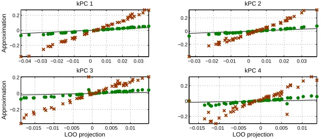
Figure 4: Approximating the leave-one-out (LOO) procedure for kPCA. We simulate a data set with four normal independent signal components, x=Σ4
k=1ηkuk+ǫ of strengths
(1.4,1.2,1.0,0.8, embedded in i.i.d. normal noiseǫ∼
N
(0,σ21), withσ=0.2. Thedi-mension was chosen D=2000 and the sample size was N=50. In the four panels we show the four kPCA component’s training set projections (red crosses), and the result of applying the point wise correction factor exp(1
c||x⊥N||2)for the lost orthogonal projection
(green dots) versus the exact LOO kPCA test projections (black).
For a coordinate-wise LOO renormalization procedure we thus propose to compute N test pro-jections by repeated kPCA on the N−1 sized sub training sets. However, compared to the PCA case we face two additional challenges, namely the potentially strongly non-Gaussian distributions and component dependencies.
To check for dependency we appeal to simple pairwise permutation test of significant mutual information measure (see, e.g., Moddemeijer, 1989). If the null hypothesis is rejected for a given set of components we cannot expect coordinate-wise renormalization to be effective. If, on the other hand, the kernel PCA projections pass the independence test we can proceed to renormalize the components individually. In the following we will assume that a coordinate-wise approach is acceptable. First, as a simple approximation to the full LOO we consider adjusting for the common scaling factor due to the lost orthogonal projection. This may indeed provide for viable approxima-tion as seen in Figure 4.
0 5 10 15 20 0
50 100 150
x
0 5 10 15 20
0 200 400 600
Sample No.
0 5 10 15 20
0 50 100 150
x
0 5 10 15 20
0 200 400 600
Sample No.
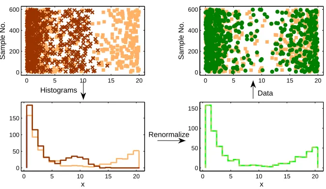
Data Histograms
Renormalize
Figure 5: Illustration of renormalization by histogram equalization. The left panel shows the train-ing set (yellow squares) and original test set (red crosses) and their respective histograms. The histograms are then equalized as seen in the right panel, where the green dots are the renormalized test data. The renormalization clearly restores the variation of the test set.
distribution, and may potentially lead to a high misclassification rate. The right panel of the figure shows how histogram equalization restores generalizability.
Technically, the transformation may be described as follows. Let H(f)be the cumulative distri-bution of values f of a given kPCA projection of the training set. Let the test set projections on the same component for Ntestsamples take values g(m). Let I(m)be the index of sample m in a sorted
list of the test set values. Then the renormalized value of the test projection m is
g
g(m) =H−1(I(m)/Ntest).
The test set projections can be obtained by the simple relation
g
g(m) = fsort(I(m)), (4)
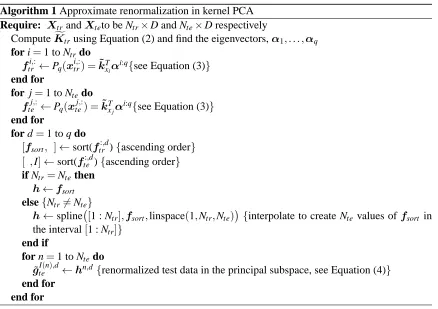
where fsortis the sorted list of training set projections. The algorithm for approximate
renormaliza-tion is summarized in Algorithm 1.2
4. Evaluation of the Proposed Cure in Classification Problems
In the following we evaluate the non-parametric exact LOO correction scheme when kPCA is used as a dimensional reduction step in simulated and real classification data sets.
Algorithm 1 Approximate renormalization in kernel PCA Require: XtrandXteto be Ntr×D and Nte×D respectively
ComputeKftrusing Equation (2) and find the eigenvectors,α1, . . . ,αq
for i=1 to Ntrdo ftri,:←Pq(xtri,:) =k˜xTiα
i:q{see Equation (3)}
end for
for j=1 to Ntedo ftej,:←Pq(xtej,:) =˜kTxjα
i:q{see Equation (3)}
end for
for d=1 to q do
[fsort, ]←sort(ftr:,d){ascending order} [ ,I]←sort(fte:,d){ascending order}
if Ntr=Ntethen h←fsort
else{Ntr6=Nte}
h←spline [1 : Ntr],fsort,linspace(1,Ntr,Nte)
{interpolate to create Nte values of fsort in
the interval[1 : Ntr]}
end if
for n=1 to Ntedo
˜
gteI(n),d←hn,d{renormalized test data in the principal subspace, see Equation (4)}
end for end for
4.1 Simulated Data
To get some insight into the non-linear regime, we design a synthetic data set containing two 2-dimensional semi-circular clusters which cannot be separated linearly (cf., Jenssen et al., 2006). Gaussian noise is added to one of the clusters, and the data is further embedded in 1000 ‘noise dimensions’. The basis is changed so that the 2D signal space occupies a general position. The noise is as earlier assumed i.i.d. with varianceσ2. The assignment variable is t=0,1, and in the experiments the data set is assumed unbalanced with p(t=0) =0.6.
In Figure 6 we show in the left panel a linear discriminant trained on the training set projections in a data set of N=500 in D=1000 dimensions. The role of the non-linearity as controlled by the parameter c in the Gaussian kernel is investigated in Figure 7 for a simulation setup similar to Figure 6. As seen the inflation problem dramatically amplifies as non-linearity increases. Finally, Figure 8 shows how renormalization improves the learning curve for the same problem.
4.2 USPS Handwritten Digit Data
The USPS handwritten digit benchmark data set is often used to illustrate unsupervised and super-vised kernel methods. The USPS data set consists of D=16×16=256 pixels handwritten digits.3 For each digit we randomly chose 10 examples for training and another 10 examples for testing. The scale was chosen as the 5th percentile of the mutual distances of the data points leading to c≈120,
−0.05 0 0.05 0.1 0.15 −0.2
−0.15 −0.1 −0.05 0 0.05
KPCA 1
KPCA 2
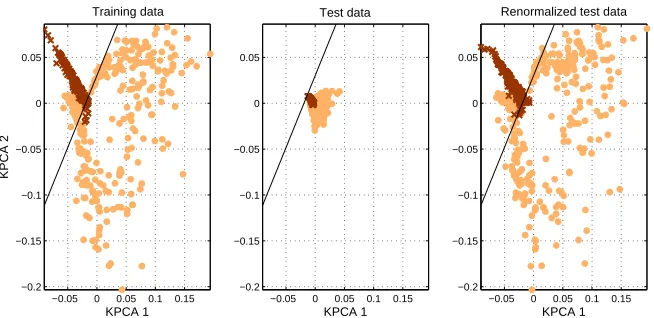
Training data
−0.05 0 0.05 0.1 0.15 −0.2
−0.15 −0.1 −0.05 0 0.05
KPCA 1 Test data
−0.05 0 0.05 0.1 0.15 −0.2
−0.15 −0.1 −0.05 0 0.05
KPCA 1 Renormalized test data
Figure 6: An unbalanced two cluster data set showing a pronounced variance inflation problem in the projections of the test data in the middle panel. In the right panel we have applied the cure based on non-parametric renormalization to equalize training and test projections us-ing histogram equalization. The linear discriminant performs close to the optimal Bayes rate after non-parametric renormalization. The sample size is N=500 in D=1000 di-mensions and the SNR is 10. The training error rate is 0.002 while the uncorrected test error rate is 0.4. Renormalization reduces the test error to 0.002.
and the number of principal components was chosen so 85% of the variance was contained in the principal subspace leading to around q=57 PCs to be included.
The first step is to submit the data to the mutual information permutation test. For every pair of principal components a permutation test with 1000 permutations was performed in order to test the null hypothesis of the two given components being independent. Using aρ=0.05 significance level, we find that the null hypothesis can only be rejected for approximately 2% of the principal component pairs when not using Bonferroni correction. The combinations for which the null hy-pothesis can be rejected are equally distributed across the principal components. Since the expected number of rejected tests at the given confidence level is 5%, hence, we can safely proceed with the coordinate-wise renormalization process.
In the q dimensional principal subspace the projections of the test set are renormalized to follow the training set histogram. We chose in these experiments for demonstration to classify digit 8 versus the rest. A linear discriminant classifier was trained on the kernel PCA projections of the training set, and the classification error was found using both the conventional kernel PCA projections of the test set and their renormalized counterparts. In order to compare the two methods, the procedure was repeated 300 times using random training and test sets. While classification based on the conventional projections resulted in a mean classification error rate (±1 std) of 0.06±0.01, using the renormalized projections lowered the error rate to 0.05±0.02. A paired t-test showed that this reduction is highly significant (p=2.0875·10−11).
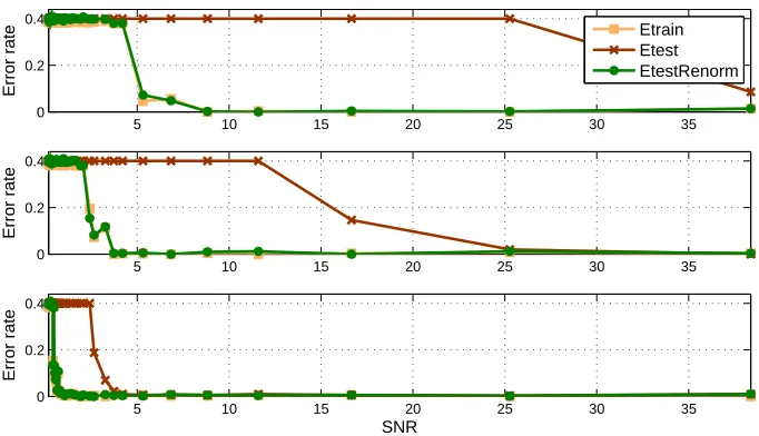
misclas-5 10 15 20 25 30 35 0
0.2 0.4
Error rate
Etrain Etest EtestRenorm
5 10 15 20 25 30 35
0 0.2 0.4
Error rate
5 10 15 20 25 30 35
0 0.2 0.4
SNR
Error rate
Figure 7: The role of non-linearity on the variance inflation problem. We carry out three experi-ments at different values of the Gaussian kernel scale parameter (top to bottom: c=0.05, c=0.1, c=0.5). We show classification errors as a function of SNR. The linear discrim-inant performs close to the optimal Bayes rate after the renormalization operation in all cases, while the un-renormalized systems suffers from poor generalizability. The sample size is N=500 and the number of dimensions is D=1000.
sification rate. The bottom row illustrates how renormalization overcomes the distortions induced by the variance inflation. The discriminant line is seen to separate the two classes appropriately.
To gain a better understanding of how the variance inflation and quality of the renormalization are effected by noise, we added Gaussian noise (
N
(0,σ2e)) withσe∈[0,5]. For every noise level,
300 random training and test sets where drawn as explained above and kPCA was performed. Once again our goal was to classify digit 8 versus the rest by a linear classifier in the principal subspace. The results are summarized in Figure 10 where we show the error rate before and after renormal-ization as well as the result based on renormalizing according to the leave-one-out error. In the last case, the N projections determined from leave-one-out cross validation (LOOCV) are renormalized to follow the entire training set histogram. Renormalization is then only applied to the test set when this renormalized LOOCV error is less than the estimated baseline error. In the right panel of Figure 10 it is seen how renormalizing the projections leads to a much improved classifier as long as the SNR is ‘reasonable’. Even whenσe=0 there is some inherent noise in the data, which explains
why renormalization still improves the classification. Asσe reaches 1 it is no longer possible to
identify the digits by visual inspection, and classification becomes increasingly difficult.
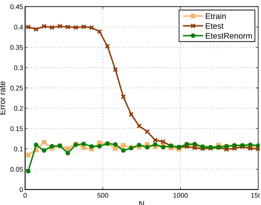
be-0 500 1000 1500 0
0.05 0.1 0.15 0.2 0.25 0.3 0.35 0.4 0.45
N
Error rate
Etrain Etest EtestRenorm
Figure 8: Classification error learning curves for the two semicircular clusters in i.i.d. noise setup. The signal to noise ratio was SNR=60. The linear discriminant performs close to the optimal Bayes rate after the renormalization operation in all cases, while the conventional system suffers from poor generalizability, and requires about ten times as many examples to reach the same error level as the renormalized classifier. The experiment was carried out with D=2000.
havior is naturally not encountered for the renormalized projections. Instead, as the SNR decreases, renormalization increases the error rate, as the test set observations are forced to be distributed on both sides of the discrimination line - which leads to many misclassifications when the signal is sup-pressed by the noise. However, using LOOCV based renormalization prevents the error rate from blowing up while at the same time improving the classification in the more sensible SNR regime as compared to conventional kPCA.
4.3 Functional MRI Data
−0.6 −0.4 −0.2 0 0.2 −0.6 −0.4 −0.2 0 0.2 00 0 0 0 0 00 0 0 1 1 1 1 1 11 1 1 1 2 22 2 2 2 2 2 2 2 3 33 3 3 3 333
3 44 4 4 4 4 4 44 4 5 5 5 5 5 555 55 6 6 6 6 6 66 6 6 67 77 7 7 7 7 77 7 8 8
88 88 8 8 8 8 9 9 9 9 9 9 9 9 9 9 kPC 3
−0.6 −0.4 −0.2 0 0.2 −0.6 −0.4 −0.2 0 0.2 00 0 0 0 000 0 0 1 1 1 1 1 1 1 1 1 1 2 22 2 2 2 2 2 2 2 3 33 3 3 3 333
3 4 4 4 4 4 4 4 4 4 4 5 5 5 5 5 5 55 55 6 6 6 6 6 6 6 6 6 6 7 7 7 7 7 7 7 7 7 7 8 8 8 8 8 8 8 8 8 8 9 9 9 9 9 9 9 9 99 kPC 3 kPC 1
−0.4 −0.2 0 0.2
−0.6 −0.4 −0.2 0 0.2 00 0 0 0 0 00 0 0 1 1 1 1 1 1 1 1 1 1 2
2222 2 2 2 2 2 3 3 3 3 3
3 3 33
3 4 4 4 4 4 4 4 4 4 4 5 55 5 5 5 5 5 55 6 6 6 6 6 66 6 6 6 7 77 7 7 7 7 7 7 7 8 8 8 8 88 8 8 8 8 9 9 9 9 9 9 9 99 9
−0.4 −0.2 0 0.2
−0.6 −0.4 −0.2 0 0.2 00 0 0 0 0 0 0 0 0 1 1 1 1 1 1 1 1 1 1 2
2222 2 2 2 2 2 3 3 3 3 3
3 3 33
3 4 4 4 4 4 4 4 4 4 4 5 55 5 5 5 5 5 55 6 6 6 6 6 66 6 6 6 7 77 7 7 7 7 7 7 7 8 8 8 8 8 8 8 8 8 8 9 9 9 9 9 9 9 99 9 kPC 2
−0.4 −0.2 0 0.2 0.4 −0.6 −0.4 −0.2 0 0.2 0 0 0
0 0 00 0 0 0 1 1 1 1 1 1 11 1 1 2 2 222
2 2 2 2 2 3 3 33 3 333 3
3 44 4 4 4 4 4 4 4 4 5 5 5 5 5 5 5 5
5 5 6 6 6 6 6 6 66 6
6 77
7 7 7 7 7 7 7 7 8 8 8 8 8 8 8 8 8 8 9 99 9 9 9 9 99 9
−0.4 −0.2 0 0.2 0.4 −0.6 −0.4 −0.2 0 0.2 0 0 0
0 0 00 0 0 0 1 1 1 1 1 1 1 1 1 1 2 2222
2 2 2 2 2 3 3 33 3 3 3 33 3 44 4 4 4 4 4 4 4 4 5 5 5 5 5 5 5 5 5 5 6 6 6 6 6 6 6 6 6 6 7 77 7 7 7 7 7 7 7 8 8 8 8 88 8 8 8 8 9 9 9 9 9 9 9 99 9 kPC 4
−0.2 0 0.2 0.4
−0.6 −0.4 −0.2 0 0.2 0 0 0 0 0 0 0 0 0 0 1 1 1 1 1 1 11 1 1 2 2 2 2 2 2 2 2 2 2 3 3333
3 3 3 3 3 4 4 4 4 4 4 4 4 4 4 5 5 5 5 5 5 5 5 55 6 6 6 66 66 6 6
6 7 7
7 7 7 7 7 77 7 8 8 8 8 88 8 8 8 8 9 99 9 9 9 9 99 9
−0.2 0 0.2 0.4
−0.6 −0.4 −0.2 0 0.2 0 0 0 0 0 0 0 0 0 0 1 1 1 1 1 1 1 1 1 1 2 2 2 2 2 2 2 2 2 2 3 3 33 3
3 3 3 3 3 4 4 4 4 4 4 4 4 4 4 5 5 5 5 5 5 5 5 55 6 6 6 6 6 66 6 6 6 7 7 7 7 7 7 7 77 7 8 8 8 8 8 8 8 8 8 8 9 9 9 9 9 9 9 99 9 kPC 5
−0.2 0 0.2 0.4
−0.6 −0.4 −0.2 0 0.2 0 0 0
0 00 0 0 0 0 1 1 1 1 1 1 1 1 1 1 2 2 2 2 2 2 2 2 2 2 3 3 3 3 3 3 3 33 3 4 4 4 4 4 4 4 4 4 4 5 5 5 5 5 55 5 55 6 6 6 6 6 6 6 6 6
6 77 7 7 7 7 7 7 7 7 8 8
8 88 8 8 8 8 8 9 9 9 9 9 9 9 99 9
−0.2 0 0.2 0.4
−0.6 −0.4 −0.2 0 0.2 0 0 0
00 0 0 0 0 0 1 1 1 1 1 1 1 1 1 1 2 2 2 2 2 2 2 2 2 2 3 3 3 3 3 3 33 3 3 4 4 4 4 4 4 4 4 4 4 5 5 5 5 5 5 5 5 55 6 6 6 6 6 6 6 6 6 6 7 77 7 7 7 7 7 7 7 8 8 8 8 8 8 8 8 8 8 9 9 9 9 9 9 9 99 9 kPC 6
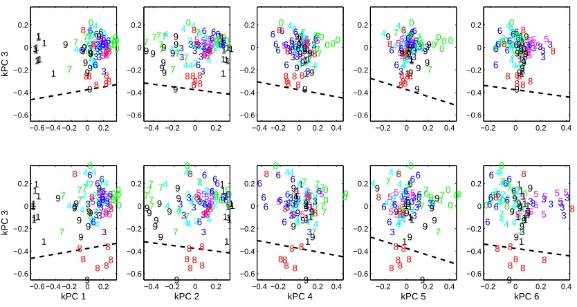
Figure 9: USPS handwritten digits test set projections. The top row shows the conventional projec-tions, while the bottom row shows the projections after renormalization. In this example the third kPC carries a large part of the signal, and hence this component is shown versus the other five first PCs. The variance reduction and the consequent shift is evident from the top row. The dashed line indicates the linear discriminant function for classifying digit 8 vs the rest.
simple on-off activation reference function for supervision of the classifier. The reference function is off-set by 4 seconds to emulate the hemodynamic delay.
The data set is split in two equal sized subsets: Five runs for training and five runs for testing. As the test and training data are independent, the test error estimate is an unbiased estimator of performance. The scale of the Gaussian kernel was chosen as the 5th percentile of the mutual distances leading to c≈15000, while the dimension of the principal subspace is chosen as q=20.
Again the principal components are tested for independence by a mutual information permuta-tion test. Using 1000 permutapermuta-tions and aρ=0.05 significance level, we find that the null hypothesis is rejected for approximately 1% of the principal component pairs.
Similar to the handwritten digit data we perform linear classification in the kernel principal subspace. This was repeated 300 times using random splits for different noise levels. The results are summarized in Figure 11. Again renormalization is seen to decrease the error rate significantly, while the LOOCV based scheme furthermore prevents the increase in error rate for high noise levels (low SNR).
0 1 2 3 4 5 0.05
0.06 0.07 0.08 0.09 0.1 0.11 0.12 0.13 0.14
Error rate
Std. of noise Etest EtestRenorm LOOCV based
0 0.2 0.4 0.6 0.8 1
0.05 0.055 0.06 0.065 0.07 0.075 0.08 0.085 0.09 0.095 0.1
Std. of noise
Figure 10: Mean error rates±1 standard deviation as a function of the noise level. The test error based on conventional kernel PCA projections, renormalized projections, and a LOOCV scheme is shown. Renormalization is seen to improve the performance, while LOOCV based renormalization prevents the classification error to blow up in the very low SNR regime.
5. Conclusion
Dimensionality reduction by PCA and kPCA can lack generalization due to training set variance inflation in the extremely ill-posed case when the sample size is much smaller than the input space dimension. In this work we have provided a simple geometric explanation for the main effect, namely that test points ‘loose’ their orthogonal projections, when their embedding is computed. This insight allowed for a speed-up of a previously proposed LOO scheme for renormalization. For kPCA we showed that the effects can be even more dramatic than in PCA, and we proposed a scheme for exact LOO renormalization of the embedding, and an approximate expression at lower cost. The viability of the new scheme was demonstrated for kPCA when used for dimensionality reduction both in simple synthetic data, in the USPS digit classification problem, and for fMRI brain state decoding.
Acknowledgments
0 5 10 15 20 25 30 0.05
0.1 0.15 0.2 0.25 0.3
Std. of noise
Error rate
Etest EtestRenorm LOOCV based
A
Figure 11: Mean error rates±1 standard deviation as a function of the noise level for fMRI data (D=16,384,N=605) . The test error based on conventional kernel PCA projections, renormalized projections, and a LOOCV scheme is shown. Renormalization is seen to clearly improve the performance. Arrow ’A’ indicates the noise level used in Figure 12
Appendix A.
LetuN,kbe the k’th eigenvector of the covariance matrix on the full sampleΣN anduN−1,k be the
corresponding eigenvector of LOO training set covariance matrixΣN−1. In the following we use
first order perturbation theory to show that
uTN−1,k·xN≈uTN,k·x k N,
where the data vectorxhas been split in its orthogonal and parallel components, xN=x⊥N+x k N,
relative to the subspace spanned by the training data. Thus, we are interested in the difference betweenuN,kanduN−1,k. Simple manipulations of the covariance matrices lead to
ΣN−1=ΣN+
1
N−1ΣN− 1
N(xN−µN−1)(xN−µN−1) T
| {z }
O(1
N)
.
By introducing the shorthandA=ΣN−1andB=ΣN we get
A=B+δC, (5)
whereδis of order N1. Note that all matrices are symmetric. We now look at the k’th eigenvector of AandB:
Buk=λkuk, (6)
−0.1 0 0.1 −0.15
−0.1 −0.05 0 0.05 0.1
kPC 1
−0.1 0 0.1 −0.15
−0.1 −0.05 0 0.05 0.1
kPC 1
kPC 2
−0.1 0 0.1 −0.15
−0.1 −0.05 0 0.05 0.1
−0.1 0 0.1 −0.15
−0.1 −0.05 0 0.05 0.1
kPC 3
−0.1 0 0.1 −0.15
−0.1 −0.05 0 0.05 0.1
−0.1 0 0.1 −0.15
−0.1 −0.05 0 0.05 0.1
kPC 4
−0.1 0 0.1 −0.15
−0.1 −0.05 0 0.05 0.1
−0.1 0 0.1 −0.15
−0.1 −0.05 0 0.05 0.1
kPC 5
−0.1 0 0.1 −0.15
−0.1 −0.05 0 0.05 0.1
−0.1 0 0.1 −0.15
−0.1 −0.05 0 0.05 0.1
kPC 6
Figure 12: Test set projections of the fMRI data with Gaussian noise added as marked on Figure 11 (εi=
N
(0,3.82)). The top row shows the conventional projections, while the bottomrow shows the projections after renormalization. The ‘red class’ indicates activation, while the blue observations are acquired during rest. The dashed line marks the linear discriminant. The scale is chosen as the 5th percentile of the mutual distances.
First order perturbation theory posits
νk=λk+δξk, (8)
vk=uk+δwk. (9)
That is, when going from N to N−1 samples we only have a small (O(N1)) change in eigenvalues and rotation of eigenvectors. Since all eigenvectors are orthonormal it follows thatuk⊥wk, c.f.,
||vk||2=||uk+δwk||2=||uk||2 | {z }
=1
+|{z}δ2
≈0
||wk||2+2δuTkwk=1
δuTkwk=0.
We now expand Equation (7) using Equation (5), (8) and (9)
Avk=νkvk ⇒
(B+δC)(uk+δwk) = (λk+δξk)(uk+δwk),
ignoring higher order terms ofδgives
Finally, exploiting Equation (6) reduces the above to
Cuk+Bwk=λkwk+ξkuk . (10)
We now look for an estimate ofξkby left multiplying withuTk
uTkCuk+uTkBwk=λkuTkwk+ξkuTkuk ,
using||uk||2=1 anduk⊥wkgives
uTkCuk+uTkBwk=ξk,
sinceB is symmetric, uk is both a left and right singular vector. Hence, uTkBwk=λkuTkwk=0.
Thus finally, it follows that
uTkCuk=ξk. (11)
Next, we find an estimate ofwkby left multiplying Equation (10) withuTj j6=k.
uTjCuk+uTjBwk=λkuTjwk+ξkuTjuk ,
again we exploit the fact thatBis symmetric and thatujis orthogonal touk, which gives
uTjCuk+λjuTjwk=λkuTjwk . (12)
Assuming that span{u1,u2, . . . ,uD}= span{v1,v2, . . . ,vD}, that is, thev-basis is a rotation of the u-basis, which implies that wk can be represented as a linear combination of the u-vectors (or v-vectors), leads to
wk= D
∑
m=1hkmum.
Due to orthonormality of the eigenvectors, we now realize that hkk=0 anduTjwk=uTj ∑Dm=1hkmum
will only be non-zero for m= j. Hence, Equation (12) reduces to
uTjCuk+λjhk j=λkhk j ⇒
hk j= uT
jCuk
λk−λj k6= j
hkk=0.
In the above we have assumed a nondegenerate system, that is,λk6=λj ∀k6= j. Thus,wk can be
expressed as
wk= N
∑
m=16=kuTmCuk
λk−λm
where we used thatCuk is only non-zero for k≤N. We are now ready to return to Equation (8)
and (9) inserting the expressions derived forξk andwkin Equation (11) and (13) respectively:
νk=λk+δuTkCuk (14)
vk=uk+δ N
∑
m=16=k(uTm(xN−µN−1))(uTk(xN−µN−1))
λk−λm
um. (15)
Equation (14) shows that the change in eigenvalue is indeed small (O(1
N)) when going from N to N−1 samples. For the eigenvector perturbation, Equation (15), we can bound the squared length of the sum and obtain a similar result,
1 N
N
∑
m=16=k(uT
m(xN−µN−1))(uTk(xN−µN−1))
λk−λm
um
2 ≤
1
N2||xN−µN−1|| 2
N
∑
m=16=k(uT
m(xN−µN−1))
λk−λm
um =
1
N2||xN−µN−1|| 2
∑
Nm=16=k
|(uT
m(xN−µN−1))|2 |λk−λm|2
≤
1 N2
2||xN−µN−1||4
|∆λk|2 ,
where∆λkis the spacing between the k’th eigenvalue and the closest neighbor, and the factor of two
compensates for the missing k’th term in the sum, that is, the perturbation is of order O(1/N)
References
Michael Biehl and Andreas Mietzner. Statistical mechanics of unsupervised structure recognition. Journal of Physics A-Mathematical and General, 27(6):1885–1897, 1994.
Gilles Blanchard, Olivier Bousquet, and Laurent Zwald. Statistical properties of kernel principal component analysis. Machine Learning, 66(2-3):259–294, 2007.
Mikio L. Braun, Joachim M. Buhmann, and Klaus-Robert M¨uller. On relevant dimensions in kernel feature spaces. Journal of Machine Learning Research, 9:1875–1908, 2008.
Rafael C. Gonzalez and Paul Wintz. Digital Image Processing. 1977. ISBN 0-201-02596-5 (hard-cover), 0-201-02597-3 (paperback).
David C. Hoyle and Magnus Rattray. A statistical mechanics analysis of gram matrix eigenvalue spectra. In Lecture Notes in Computer Science, 17th Annual Conference on Learning Theory, volume 3120, pages 579–593. Springer Verlag, 2004a.
David C. Hoyle and Magnus Rattray. Principal-component-analysis eigenvalue spectra from data with symmetry-breaking structure. Physical Review E, 69(2):026124, 2004c.
David C. Hoyle and Magnus Rattray. Statistical mechanics of learning multiple orthogonal signals: Asymptotic theory and fluctuation effects. Physical Review E (Statistical, Nonlinear, and Soft Matter Physics), 75(1):016101, 2007.
Jonathan J . Hull. A database for handwritten text recognition research. IEEE Transactions on Pattern Analysis and Machine Intelligence, 16(5):550–554, 1994.
Robert Jenssen, Torbj¨orn Eltoft, Deniz Erdogmus, and Jose C. Principe. Some equivalences between kernel methods and information theoretic methods. Journal of VLSI Signal Processing, 45:49–65, 2006.
Iain M. Johnstone. On the distribution of the largest eigenvalue in principal components analysis. Annals of Statistics, 29(2):295–327, 2001.
Ulrik Kjems, Lars K. Hansen, and Stephen C. Strother. Generalizable singular value decomposition for ill-posed datasets. In Advances in Neural Information Processing Systems 13, pages 549–555. MIT Press, 2001.
Rudy Moddemeijer. On estimation of entropy and mutual information of continuous distributions. Signal Processing, 16(3):233–246, 1989.
Sofia Mosci, Lorenzo Rosasco, and Alessandro Verri. Dimensionality reduction and generalization. In Proceedings of the 24th International Conference on Machine Learning, pages 657–664, 2007.
Peter Reimann, Chris Van den Broeck, and Geert J. Bex. A Gaussian scenario for unsupervised learning. Journal of Physics A - Mathematical and General, 29(13):3521–3535, 1996.
Bernhard Sch¨olkopf, Alex Smola, and Klaus-Robert M¨uller. Nonlinear component analysis as a kernel eigenvalue problem. Neural Computation, 10(5):1299–1319, 1998.
John Shawe-Taylor and Christopher K. I. Williams. The stability of kernel principal components analysis and its relation to the process eigenspectrum. In Advances in Neural Information Pro-cessing Systems 15, pages 367–374. MIT Press, 2003.
Jack W. Silverstein and Patrick L. Combettes. Signal-detection via spectral theory of large dimen-sional random matrices. IEEE Transactions on Signal Processing, 40(8):2100–2105, 1992.