Convergence Rates of Efficient Global Optimization Algorithms
Adam D. Bull [email protected]
Statistical Laboratory University of Cambridge Cambridge, CB3 0WB, UK
Editor: Manfred Opper
Abstract
In the efficient global optimization problem, we minimize an unknown function f , using as few ob-servations f(x)as possible. It can be considered a continuum-armed-bandit problem, with noiseless data, and simple regret. Expected-improvement algorithms are perhaps the most popular methods for solving the problem; in this paper, we provide theoretical results on their asymptotic behaviour. Implementing these algorithms requires a choice of Gaussian-process prior, which determines an associated space of functions, its reproducing-kernel Hilbert space (RKHS). When the prior is fixed, expected improvement is known to converge on the minimum of any function in its RKHS. We provide convergence rates for this procedure, optimal for functions of low smoothness, and describe a modified algorithm attaining optimal rates for smoother functions.
In practice, however, priors are typically estimated sequentially from the data. For standard estimators, we show this procedure may never find the minimum of f . We then propose alternative estimators, chosen to minimize the constants in the rate of convergence, and show these estimators retain the convergence rates of a fixed prior.
Keywords: convergence rates, efficient global optimization, expected improvement,
continuum-armed bandit, Bayesian optimization
1. Introduction
Suppose we wish to minimize a continuous function f : X→R, where X is a compact subset ofRd.
Observing f(x)is costly (it may require a lengthy computer simulation or physical experiment), so we wish to use as few observations as possible. We know little about the shape of f ; in particular we will be unable to make assumptions of convexity or unimodality. We therefore need a global optimization algorithm, one which attempts to find a global minimum.
Many standard global optimization algorithms exist, including genetic algorithms, multistart, and simulated annealing (Pardalos and Romeijn, 2002), but these algorithms are designed for func-tions that are cheap to evaluate. When f is expensive, we need an efficient algorithm, one which will choose its observations to maximize the information gained.
We can consider this a continuum-armed-bandit problem (Srinivas et al., 2010, and references therein), with noiseless data, and loss measured by the simple regret (Bubeck et al., 2009). At time n, we choose a design point xn∈X , make an observation zn= f(xn), and then report a point x∗n
where we believe f(x∗n) will be low. Our goal is to find a strategy for choosing the xn and x∗n, in
terms of previous observations, so as to minimize f(x∗n).
would be to fix a sequence of xn in advance, and set x∗n=arg min ˆfn, for some approximation ˆfn
to f . We will show that if ˆfn converges in supremum norm at the optimal rate, then f(x∗n) also
converges at its optimal rate. However, while this strategy gives a good worst-case bound, on average it is clearly a poor method of optimization: the design points xnare completely independent
of the observations zn.
We may therefore ask if there are more efficient methods, with better average-case performance, that nevertheless provide good guarantees of convergence. The difficulty in designing such a method lies in the trade-off between exploration and exploitation. If we exploit the data, observing in regions where f is known to be low, we will be more likely to find the optimum quickly; however, unless we explore every region of X , we may not find it at all (Macready and Wolpert, 1998).
Initial attempts at this problem include work on Lipschitz optimization (summarized in Hansen et al., 1992) and the DIRECT algorithm (Jones et al., 1993), but perhaps the best-known strategy is expected improvement. It is sometimes called Bayesian optimization, and first appeared in Moˇckus (1974) as a Bayesian decision-theoretic solution to the problem. Contemporary computers were not powerful enough to implement the technique in full, and it was later popularized by Jones et al. (1998), who provided a computationally efficient implementation. More recently, it has also been called a knowledge-gradient policy by Frazier et al. (2009). Many extensions and alterations have been suggested by further authors; a good summary can be found in Brochu et al. (2010).
Expected improvement performs well in experiments (Osborne, 2010, §9.5), but little is known about its theoretical properties. The behaviour of the algorithm depends crucially on the Gaussian process priorπchosen for f . Each prior has an associated space of functions
H
, its reproducing-kernel Hilbert space.H
contains all functions X→Ras smooth as a posterior mean of f , and isthe natural space in which to study questions of convergence.
Vazquez and Bect (2010) show that whenπis a fixed Gaussian process prior of finite smooth-ness, expected improvement converges on the minimum of any f ∈
H
, and almost surely for f drawn fromπ. Grunewalder et al. (2010) bound the convergence rate of a computationally infea-sible version of expected improvement: for priorsπof smoothnessν, they show convergence at a rate O∗(n−(ν∧0.5)/d)on f drawn fromπ. We begin by bounding the convergence rate of the feasiblealgorithm, and show convergence at a rate O∗(n−(ν∧1)/d) on all f ∈
H
. We go on to show that a modification of expected improvement converges at the near-optimal rate O∗(n−ν/d).For practitioners, however, these results are somewhat misleading. In typical applications, the prior is not held fixed, but depends on parameters estimated sequentially from the data. This process ensures the choice of observations is invariant under translation and scaling of f , and is believed to be more efficient (Jones et al., 1998, §2). It has a profound effect on convergence, however: Locatelli (1997, §3.2) shows that, for a Brownian motion prior with estimated parameters, expected improvement may not converge at all.
We extend this result to more general settings, showing that for standard priors with estimated parameters, there exist smooth functions f on which expected improvement does not converge. We then propose alternative estimates of the prior parameters, chosen to minimize the constants in the convergence rate. We show that these estimators give an automatic choice of parameters, while retaining the convergence rates of a fixed prior.
Table 1 summarizes the notation used in this paper. We say f :Rd →Ris a bump function if
f is infinitely differentiable and of compact support, and f :Rd→Cis Hermitian if f(x) =f(−x).
f/g→1, we say f ∼g. Finally, if f and g are random, andP(sup|f/g| ≤M)→1 as M→∞, we
say f =Op(g).
In Section 2, we briefly describe the expected-improvement algorithm, and detail our assump-tions on the priors used. We state our main results in Section 3, and discuss implicaassump-tions for further work in Section 4. Finally, we give proofs in Appendix A.
2. Expected Improvement
Suppose we wish to minimize an unknown function f , choosing design points xn and estimated
minima x∗n as in the introduction. If we pick a prior distributionπ for f , representing our beliefs about the unknown function, we can describe this problem in terms of decision theory. Let(Ω,
F
,P)be a probability space, equipped with a random process f having lawπ. A strategy u is a collection of random variables (xn), (x∗n) taking values in X . Set zn:= f(xn), and define the filtration
F
n:=σ(xi,zi : i≤n). The strategy u is valid if xn is conditionally independent of f given
F
n−1, and likewise x∗n givenF
n. (Note that we allow random strategies, provided they do not depend on unknown information about f .)When taking probabilities and expectations we will writePuπandEuπ, denoting the dependence
on both the priorπ and strategy u. The average-case performance at some future time N is then given by the expected loss,
Euπ[f(x∗N)−min f],
and our goal, givenπ, is to choose the strategy u to minimize this quantity.
2.1 Bayesian Optimization
For N>1 this problem is very computationally intensive (Osborne, 2010, §6.3), but we can solve a simplified version of it. First, we restrict the choice of x∗nto the previous design points x1, . . . ,xn.
(In practice this is reasonable, as choosing an x∗nwe have not observed can be unreliable.) Secondly, rather than finding an optimal strategy for the problem, we derive the myopic strategy: the strategy which is optimal if we always assume we will stop after the next observation. This strategy is sub-optimal (Ginsbourger et al., 2008, §3.1), but performs well, and greatly simplifies the calculations involved.
In this setting, given
F
n, if we are to stop at time n we should choose x∗n:=xi∗n, where i∗n:=
arg min1,...,nzi. (In the case of ties, we may pick any minimizing i∗n.) We then suffer a loss z∗n−min f ,
where z∗n:=zi∗
n. Were we to observe at xn+1before stopping, the expected loss would be Euπ[z∗n+1−min f |
F
n],so the myopic strategy should choose xn+1to minimize this quantity. Equivalently, it should maxi-mize the expected improvement over the current loss,
EIn(xn+1;π):=Euπ[z∗n−z∗n+1|
F
n] =Euπ[(z∗n−zn+1)+|F
n], (1)where x+=max(x,0).
So far, we have merely replaced one optimization problem with another. However, for suitable priors, EIn can be evaluated cheaply, and thus maximized by standard techniques. The
Section 1
f unknown function X →Rto be minimized
X compact subset ofRd to minimize over
d number of dimensions to minimize over xn points in X at which f is observed
zn observations zn= f(xn)of f
x∗n estimated minimum of f , given z1, . . . ,zn
Section 2.1
π prior distribution for f u strategy for choosing xn, x∗n
F
n filtrationF
n=σ(xi,zi: i≤n)z∗n best observation z∗n=mini=1,...,nzi
EIn expected improvement given
F
nSection 2.2
µ,σ2 global mean and variance of Gaussian-process priorπ K underlying correlation kernel forπ
Kθ correlation kernel forπwith length-scalesθ ν,α smoothness parameters of K
ˆµn, ˆfn, s2n, ˆR2n quantities describing posterior distribution of f given
F
nSection 2.3
EI(π) expected improvement strategy with fixed prior ˆ
σ2
n, ˆθn estimates of prior parametersσ2,θ
cn rate of decay of ˆσ2n
θL,θU bounds on ˆθ n
EI(πˆ) expected improvement strategy with estimated prior
Section 3.1
H
θ(S) reproducing-kernel Hilbert space of Kθon S Hs(D) Sobolev Hilbert space of order s on DSection 3.2
Ln loss suffered over an RKHS ball after n steps
Section 3.3
EI(π˜) expected improvement strategy with robust estimated prior
Section 3.4
EI(·,ε) ε-greedy expected improvement strategies
2.2 Gaussian Process Models
We still need to choose a priorπfor f . Typically, we model f as a stationary Gaussian process: we consider the values f(x)to be jointly Gaussian, with mean and covariance
Eπ[f(x)] =µ, Covπ[f(x),f(y)] =σ2Kθ(x−y). (2)
µ∈Ris the global mean of f ; we place a flat prior on µ, reflecting our uncertainty over the location
of f .
σ>0 is the global scale of variation of f , and Kθ:Rd→Rits correlation kernel, governing the
local properties of f . In the following, we will consider kernels
Kθ(t1, . . . ,td):=K(t1/θ1, . . . ,td/θd), (3)
for an underlying kernel K with K(0) =1. (Note that we can always satisfy this condition by suitably scaling K andσ.) Theθi>0 are the length-scales of the process: two values f(x)and f(y)
will be highly correlated if each xi−yi is small compared with θi. For now, we will assume the
parametersσandθare fixed in advance.
For (2) and (3) to define a consistent Gaussian process, K must be a symmetric positive-definite function. We will also make the following assumptions.
Assumption 1. K is continuous and integrable.
K thus has Fourier transform
b
K(ξ):=
Z
Rde
−2πihx,ξiK(x)dx,
and by Bochner’s theorem,K is non-negative and integrable.b
Assumption 2. K is isotropic and radially non-increasing.b
In other words,Kb(x) =bk(kxk)for a non-increasing functionbk :[0,∞)→[0,∞); as a consequence, K is isotropic.
Assumption 3. As x→∞, either:
(i) Kb(x) =Θ(kxk−2ν−d)for someν>0; or
(ii) Kb(x) =O(kxk−2ν−d)for allν>0 (we will then say thatν=∞). Note the conditionν>0 is required forK to be integrable.b
Assumption 4. K is Ck, for k the largest integer less than 2ν, and at the origin, K has k-th order Taylor approximation Pk satisfying
|K(x)−Pk(x)|=O
Whenα=0, this is just the condition that K be 2ν-H¨older at the origin; when α>0, we instead require this condition up to a log factor.
The rateνcontrols the smoothness of functions from the prior: almost surely, f has continuous derivatives of any order k<ν(Adler and Taylor, 2007, §1.4.2). Popular kernels include the Mat´ern class,
Kν(x):= 2 1−ν Γ(ν)
√
2νkxk
ν kν
√
2νkxk
, ν∈(0,∞),
where kνis a modified Bessel function of the second kind, and the Gaussian kernel,
K∞(x):=e−12kxk 2
,
obtained in the limitν→∞(Rasmussen and Williams, 2006, §4.2). Between them, these kernels cover the full range of smoothness 0<ν≤∞. Both kernels satisfy Assumptions 1–4 for theνgiven; α=0 except for the Mat´ern kernel withν∈N, whereα=1
2 (Abramowitz and Stegun, 1965, §9.6). Having chosen our prior distribution, we may now derive its posterior. We find
f(x)|z1, . . . ,zn∼N ˆfn(x;θ),σ2s2n(x;θ)
,
where
ˆµn(θ):=
1TV−1z
1TV−11, (4)
ˆ
fn(x;θ):=ˆµn+vTV−1(z−ˆµn1), (5)
and
s2n(x;θ):=1−vTV−1v+(1−1
TV−1v)2
1TV−11 , (6)
for z= (zi)ni=1, V = (Kθ(xi−xj))ni,j=1, and v= (Kθ(x−xi))ni=1(Santner et al., 2003, §4.1.3). Equiv-alently, these expressions are the best linear unbiased predictor of f(x)and its variance, as given in Jones et al. (1998, §2). We will also need the reduced sum of squares,
ˆ
R2n(θ):= (z−ˆµn1)TV−1(z−ˆµn1). (7)
2.3 Expected Improvement Strategies
Under our assumptions onπ, we may now derive an analytic form for (1), as in Jones et al. (1998, §4.1). We obtain
EIn(xn+1;π) =ρ z∗n−fˆn(xn+1;θ),σsn(xn+1;θ), (8)
where
ρ(y,s):=
(
yΦ(y/s) +sϕ(y/s), s>0,
max(y,0), s=0, (9)
andΦandϕare the standard normal distribution and density functions respectively.
For a priorπas above, expected improvement chooses xn+1to maximize (8), but this does not fully define the strategy. Firstly, we must describe how the strategy breaks ties, when more than one x∈X maximizes EIn. In general, this will not affect the behaviour of the algorithm, so we allow
Secondly, we must say how to choose x1, as the above expressions are undefined when n=0. In fact, Jones et al. (1998, §4.2) find that expected improvement can be unreliable given few data points, and recommend that several initial design points be chosen in a random quasi-uniform ar-rangement. We will therefore assume that until some fixed time k, points x1, . . . ,xk are instead
chosen by some (potentially random) method independent of f . We thus obtain the following strat-egy.
Definition 1. An EI(π)strategy chooses:
(i) initial design points x1, . . . ,xkindependently of f ; and
(ii) further design points xn+1(n≥k)from the maximizers of (8).
So far, we have not considered the choice of parametersσandθ. While these can be fixed in advance, doing so requires us to specify characteristic scales of the unknown function f , and causes expected improvement to behave differently on a rescaling of the same function. We would prefer an algorithm which could adapt automatically to the scale of f .
A natural approach is to take maximum likelihood estimates of the parameters, as recommended by Jones et al. (1998, §2). Given θ, the MLE ˆσ2n=Rˆ2
n(θ)/n; for full generality, we will allow
any choice ˆσ2n=cnRˆ2n(θ), where cn =o(1/log n). Estimates ofθ, however, must be obtained by
numerical optimization. Asθ can vary widely in scale, this optimization is best performed over logθ; as the likelihood surface is typically multimodal, this requires the use of a global optimizer. We must therefore place (implicit or explicit) bounds on the allowed values of logθ. We have thus described the following strategy.
Definition 2. Let ˆπnbe a sequence of priors, with parameters ˆσn, ˆθnsatisfying:
(i) ˆσ2n=cnRˆ2n(θˆn)for constants cn>0, cn=o(1/log n); and
(ii) θL≤θˆ
n≤θU for constantsθL,θU∈Rd+.
An EI(πˆ)strategy satisfies Definition 1, replacingπwith ˆπnin (8).
3. Convergence Rates
To discuss convergence, we must first choose a smoothness class for the unknown function f . Each kernel Kθis associated with a space of functions
H
θ(X), its reproducing-kernel Hilbert space (RKHS) or native space.H
θ(X) contains all functions X →Ras smooth as a posterior mean off , and is the natural space to study convergence of expected-improvement algorithms, allowing a tractable analysis of their asymptotic behaviour.
3.1 Reproducing-Kernel Hilbert Spaces
Given a symmetric positive-definite kernel K onRd, set k
x(t) =K(t−x). For S⊆Rd, let
E
(S)bethe space of functions S→Rspanned by the kx, for x∈S. Furnish
E
(S)with the inner productdefined by
The completion of
E
(S)under this inner product is the reproducing-kernel Hilbert spaceH
(S)of K on S. The members f∈H
(S)are abstract objects, but we can identify them with functions f : S→Rthrough the reproducing property,
f(x) =hf,kxi,
which holds for all f ∈
E
(S). See Aronszajn (1950), Berlinet and Thomas-Agnan (2004), Wendland (2005) and van der Vaart and van Zanten (2008).We will find it convenient also to use an alternative characterization of
H
(S). We begin by describingH
(Rd)in terms of Fourier transforms. Let bf denote the Fourier transform of a functionf ∈L2. The following result is stated in Parzen (1963, §2), and proved in Wendland (2005, §10.2); we give a short proof in Appendix A.
Lemma 1.
H
(Rd)is the space of real continuous f ∈L2(Rd)whose norm kfk2H(Rd):=Z |bf(ξ)|2
b
K(ξ) dξ
is finite, taking 0/0=0.
We may now describe
H
(S)in terms ofH
(Rd).Lemma 2 (Aronszajn, 1950, §1.5).
H
(S)is the space of functions f =g|S for some g∈H
(Rd),with norm
kfkH(S):= inf
g|S=fk
gkH(Rd),
and there is a unique g minimizing this expression.
These spaces are in fact closely related to the Sobolev Hilbert spaces of functional analysis. Say a domain D⊆Rdis Lipschitz if its boundary is locally the graph of a Lipschitz function (see Tartar,
2007, §12, for a precise definition). For such a domain D, the Sobolev Hilbert space Hs(D)is the space of functions f : D→R, given by the restriction of some g :Rd→R, whose norm
kfk2Hs(D):= inf g|D=f
Z |gb(ξ)|2 (1+kξk2)s/2dξ
is finite. Thus, for the kernel K with Fourier transformKb(ξ) = (1+kξk2)s/2, this is just the RKHS
H
(D). More generally, if K satisfies our assumptions withν<∞, these spaces are equivalent in the sense of normed spaces: they contain the same functions, and have normsk·k1,k·k2satisfyingCkfk1≤ kfk2≤C′kfk1, for constants 0<C≤C′.
Lemma 3. Let
H
θ(S)denote the RKHS of Kθon S, and D⊆Rd be a Lipschitz domain.(i) Ifν<∞,
H
θ(D¯)is equivalent to the Sobolev Hilbert space Hν+d/2(D). (ii) Ifν=∞,H
θ(D¯)is continuously embedded in Hs(D)for all s.Thus ifν<∞, and X is, say, a product of intervals∏di=1[ai,bi], the RKHS
H
θ(X)is equivalentto the Sobolev Hilbert space Hν+d/2(∏id=1(ai,bi)), identifying each function in that space with its
3.2 Fixed Parameters
We are now ready to state our main results. Let X ⊂Rd be compact with non-empty interior. For
a function f : X→R, letPu
f andEuf denote probability and expectation when minimizing the fixed
function f with strategy u. (Note that while f is fixed, u may be random, so its performance is still probabilistic in nature.) We define the loss suffered over the ball BR in
H
θ(X) after n steps by astrategy u,
Ln(u,
H
θ(X),R):= supkfkHθ(X)≤R
Euf[f(x∗n)−min f].
We will say that u converges on the optimum at rate rn, if
Ln(u,
H
θ(X),R) =O(rn)for all R>0. Note that we do not allow u to vary with R; the strategy must achieve this rate without prior knowledge ofkfkHθ(X).
We begin by showing that the minimax rate of convergence is n−ν/d.
Theorem 1. Ifν<∞, then for anyθ∈Rd+, R>0,
inf
u Ln(u,
H
θ(X),R) =Θ(n−ν/d),
and this rate can be achieved by a strategy u not depending on R.
The upper bound is provided by a naive strategy as in the introduction: we fix a quasi-uniform sequence xnin advance, and take x∗n to minimize a radial basis function interpolant of the data. As
remarked previously, however, this naive strategy is not very satisfying; in practice it will be outper-formed by any good strategy varying with the data. We may thus ask whether more sophisticated strategies, with better practical performance, can still provide good worst-case bounds.
One such strategy is the EI(π)strategy of Definition 1. We can show this strategy converges at least at rate n−(ν∧1)/d, up to log factors.
Theorem 2. Letπbe a prior with length-scalesθ∈Rd+. For any R>0,
Ln(EI(π),
H
θ(X),R) =(
O(n−ν/d(log n)α), ν≤1,
O(n−1/d), ν>1.
Forν≤1, these rates are near-optimal. Forν>1, we are faced with a more difficult problem; we discuss this in more detail in Section 3.4.
3.3 Estimated Parameters
x f(x)
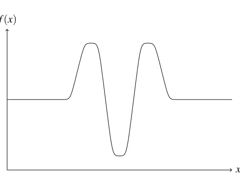
Figure 1: A counterexample from Theorem 3
Theorem 3. Suppose ν<∞. Given θ∈Rd
+, R >0, ε>0, there exists f ∈
H
θ(X) satisfyingkfkHθ(X)≤R, and for some fixedδ>0,
PEI(πˆ) f
inf
n f(x
∗
n)−min f ≥δ
>1−ε.
The counterexamples constructed in the proof of the theorem may be difficult to minimize, but they are not badly-behaved (Figure 1). A good optimization strategy should be able to minimize such functions, and we must ask why expected improvement fails.
We can understand the issue by considering the constant in Theorem 2. Define
τ(x):=xΦ(x) +ϕ(x).
From the proof of Theorem 2, the dominant term in the convergence rate has constant
C(R+σ) τ(R/σ)
τ(−R/σ), (10)
for C>0 not depending on R orσ. In Appendix A, we will prove the following result.
Corollary 1. ˆRn(θ)is non-decreasing in n, and bounded above bykfkHθ(X).
Hence for fixedθ, the estimate ˆσ2
n=Rˆ2n(θ)/n≤R2/n, and thus R/σˆn≥n1/2. Inserting this choice
into (10) gives a constant growing exponentially in n, destroying our convergence rate.
To resolve the issue, we will instead try to pickσto minimize (10). The term R+σis increasing inσ, and the termτ(R/σ)/τ(−R/σ)is decreasing inσ; we may balance the terms by takingσ=R. The constant is then proportional to R, which we may minimize by taking R=kfkHθ(X). In practice, we will not knowkfkHθ(X)in advance, so we must estimate it from the data; from Corollary 1, a convenient estimate is ˆRn(θ).
Suppose, then, that we make some bounded estimate ˆθnofθ, and set ˆσ2n=Rˆ2n(θˆn). As Theorem 3
(We may also chooseθto minimize (10); we might then pick ˆθnminimizing ˆRn(θ)∏di=1θ− ν/d i ,but
our assumptions on ˆθnare weak enough that we need not consider this further.)
If we believe our Gaussian-process model, this estimate ˆσn is certainly unusual. We should,
however, take care before placing too much faith in the model. The function in Figure 1 is a rea-sonable function to optimize, but as a Gaussian process it is highly atypical: there are intervals on which the function is constant, an event which in our model occurs with probability zero. If we want our algorithm to succeed on more general classes of functions, we will need to choose our parameter estimates appropriately.
To obtain good rates, we must add a further condition to our strategy. If z1=···=zn, EIn(·; ˆπn)
is identically zero, and all choices of xn+1are equally valid. To ensure we fully explore f , we will therefore require that when our strategy is applied to a constant function f(x) =c, it produces a sequence xndense in X . (This can be achieved, for example, by choosing xn+1uniformly at random from X when z1=···=zn.) We have thus described the following strategy.
Definition 3. An EI(π˜)strategy satisfies Definition 2, except:
(i) we instead set ˆσ2n=Rˆ2n(θˆn); and
(ii) we require the choice of xn+1maximizing (8) to be such that, if f is constant, the design points are almost surely dense in X .
We cannot now prove a convergence result uniform over balls in
H
θ(X), as the rate of conver-gence depends on the ratio R/Rˆn, which is unbounded. (Indeed, any estimator of kfkHθ(X) must
sometimes perform poorly: f can appear from the data to have arbitrarily small norm, while in fact having a spike somewhere we have not yet observed.) We can, however, provide the same convergence rates as in Theorem 2, in a slightly weaker sense.
Theorem 4. For any f ∈
H
θU(X), underPEIf (π˜),f(x∗n)−min f =
(
Op(n−ν/d(log n)α), ν≤1,
Op(n−1/d), ν>1.
3.4 Near-Optimal Rates
So far, our rates have been near-optimal only forν≤1. To obtain good rates forν>1, standard results on the performance of Gaussian-process interpolation (Narcowich et al., 2003, §6) then require the design points xi to be quasi-uniform in a region of interest. It is unclear whether this
occurs naturally under expected improvement, but there are many ways we can modify the algorithm to ensure it.
Perhaps the simplest, and most well-known, is an ε-greedy strategy (Sutton and Barto, 1998, §2.2). In such a strategy, at each step with probability 1−εwe make a decision to maximize some greedy criterion; with probabilityεwe make a decision completely at random. This random choice ensures that the short-term nature of the greedy criterion does not overshadow our long-term goal.
The parameterεcontrols the trade-off between global and local search: a good choice ofεwill be small enough to not interfere with the expected-improvement algorithm, but large enough to prevent it from getting stuck in a local minimum. Sutton and Barto (1998, §2.2) consider the values ε=0.1 andε=0.01, but in practical workεshould of course be calibrated to a typical problem set.
Definition 4. Let·denoteπ, ˆπor ˜π. For 0<ε<1, an EI(·,ε)strategy:
(i) chooses initial design points x1,···,xkindependently of f ;
(ii) with probability 1−ε, chooses design point xn+1(n≥k)as in EI(·); or (iii) with probabilityε, chooses xn+1(n≥k)uniformly at random from X .
We can show that these strategies achieve near-optimal rates of convergence for allν<∞.
Theorem 5. Let EI(·,ε)be one of the strategies in Definition 4. Ifν<∞, then for any R>0,
Ln(EI(·,ε),
H
θU(X),R) =O((n/log n)−ν/d(log n)α),while ifν=∞, the statement holds for allν<∞.
Note that unlike a typicalε-greedy algorithm, we do not rely on random choice to obtain global convergence: as above, the EI(π)and EI(π˜)strategies are already globally convergent. Instead, we use random choice simply to improve upon the worst-case rate. Note also that the result does not in general hold whenε=1; to obtain good rates, we must combine global search with inference about
f .
4. Conclusions
We have shown that expected improvement can converge near-optimally, but a naive implementation may not converge at all. We thus echo Diaconis and Freedman (1986) in stating that, for infinite-dimensional problems, Bayesian methods are not always guaranteed to find the right answer; such guarantees can only be provided by considering the problem at hand.
We might ask, however, if our framework can also be improved. Our upper bounds on conver-gence were established using naive algorithms, which in practice would prove inefficient. If a so-phisticated algorithm fails where a naive one succeeds, then the soso-phisticated algorithm is certainly at fault; we might, however, prefer methods of evaluation which do not consider naive algorithms so successful.
Vazquez and Bect (2010) and Grunewalder et al. (2010) consider a more Bayesian formulation of the problem, where the unknown function f is distributed according to the prior π, but this approach can prove restrictive: as we saw in Section 3.3, placing too much faith in the prior may exclude functions of interest. Further, Grunewalder et al. find the same issues are present also within the Bayesian framework.
A more interesting approach is given by the continuum-armed-bandit problem (Srinivas et al., 2010, and references therein). Here the goal is to minimize the cumulative regret,
Rn:= n
∑
i=1(f(xi)−min f),
in general observing the function f under noise. Algorithms controlling the cumulative regret at rate rnalso solve the optimization problem, at rate rn/n (Bubeck et al., 2009, §3). The naive algorithms
is necessarily increasing, so cannot establish rates of optimization faster than n−1. (This is not an issue under noise, where typically rn=Ω(n1/2), see Kleinberg and Slivkins, 2010.) Secondly, if our
goal is optimization, then minimizing the regret, a cost we do not incur, may obscure the problem at hand.
Bubeck et al. (2010) study this problem with the additional assumption that f has finitely many minima, and is, say, quadratic in a neighbourhood of each. This assumption may suffice in practice, and allows the authors to obtain impressive rates of convergence. For optimization, however, a further weakness is that these rates hold only once the algorithm has found a basin of attraction; they thus measure local, rather than global, performance. It may be that convergence rates alone are not sufficient to capture the performance of a global optimization algorithm, and the time taken to find a basin of attraction is more relevant. In any case, the choice of an appropriate framework to measure performance in global optimization merits further study.
Finally, we should also ask how to choose the smoothness parameterν(or the equivalent pa-rameter in similar algorithms). Van der Vaart and van Zanten (2009) show that Bayesian Gaussian-process models can, in some contexts, automatically adapt to the smoothness of an unknown func-tion f . Their technique requires, however, that the estimated length-scales ˆθn to tend to 0, posing
both practical and theoretical challenges. The question of how best to optimize functions of un-known smoothness remains open.
Acknowledgments
We would like to thank the referees, as well as Richard Nickl and Steffen Grunewalder, for their valuable comments and suggestions.
Appendix A. Proofs
We now prove the results in Section 3.
A.1 Reproducing-Kernel Hilbert Spaces
Proof of Lemma 1. Let V be the space of functions described, and W be the closed real subspace of Hermitian functions in L2(Rd,Kb−1). We will show f 7→ bf is an isomorphism V →W , so we may
equivalently work with W . Given bf∈W , by Cauchy-Schwarz and Bochner’s theorem,
Z
|bf| ≤
Z
b
K
1/2Z
|bf|2/Kb
1/2 <∞,
and askKbk∞≤ kKk1,
Z
|bf|2≤ kKbk∞
Z
|bf|2/Kb<∞,
f7→ bf is hence an isomorphism V →W . It remains to show that V =
H
(Rd). W is complete, soV is. Further,
E
(Rd)⊂V , and by Fourier inversion each f ∈V satisfies the reproducing property,f(x) =
Z
e2πihx,ξibf(ξ)dξ=
Z bf(ξ)bk
x(ξ)
b
K(ξ) dξ=hf,kxi,
so
H
(Rd) is a closed subspace of V . Given f ∈H
(Rd)⊥, f(x) =hf,kxi=0 for all x, so f =0. Thus V =H
(Rd).Proof of Lemma 3. By Lemma 1, the norm on
H
θ(Rd)iskfk2Hθ(Rd)=
Z |bf(ξ)|2
b
Kθ(ξ) dξ,
and Kθhas Fourier transform
b
Kθ(ξ) =Kb(ξ1/θ1, . . . ,ξd/θd)
∏d i=1θi
.
Ifν<∞, by assumptionKb(ξ) =bk(kξk), for a finite non-increasing functionbk satisfyingbk(kξk) =
Θ(kξk−2ν−d)asξ→∞. Hence
C(1+kξk2)−(ν+d/2)≤Kbθ(ξ)≤C′(1+kξk2)−(ν+d/2),
for constants C,C′>0, and we obtain that
H
θ(Rd)is equivalent to the Sobolev space Hν+d/2(Rd).From Lemma 2,
H
θ(D)is given by the restriction of functions inH
θ(Rd); as D is Lipschitz, thesame is true of Hν+d/2.
H
θ(D) is thus equivalent to Hν+d/2(D). Finally, functions inH
θ(D¯) are continuous, so uniquely identified by their restriction to D, andH
θ(D¯)≃H
θ(D)≃Hν+d/2(D).Ifν=∞, by a similar argument
H
θ(D¯)is continuously embedded in all Hs(D).From Lemma 1, we can derive results on the behaviour ofkfkHθ(S)asθvaries. For smallθ, we obtain the following result.
Lemma 4. If f ∈
H
θ(S), then f ∈H
θ′(S)for all 0<θ′≤θ, andkfk2H
θ′(S)≤
d
∏
i=1θi/θ′i
!
kfk2Hθ(S).
Proof. Let C=∏d
i=1(θ′i/θi). AsK is isotropic and radially non-increasing,b
b
Kθ′(ξ) =CKbθ((θ′1/θ1)ξ1, . . . ,(θ′d/θd)ξd)≥CKbθ(ξ).
Given f ∈
H
θ(S), let g∈H
θ(Rd)be its minimum norm extension, as in Lemma 2. By Lemma 1,kfk2Hθ′(S)≤ kgk
2
Hθ′(Rd)=
Z
|gb|2 b
Kθ′ ≤
Z
|bg|2 CKbθ =C
−1
Likewise, for largeθ, we obtain the following.
Lemma 5. Ifν<∞, f ∈
H
θ(S), then f ∈H
tθ(S)for t≥1, andkfk2H
tθ(S)≤C
′′t2νkfk2
Hθ(S),
for a C′′>0 depending only on K andθ.
Proof. As in the proof of Lemma 3, we have constants C,C′>0 such that
C(1+kξk2)−(ν+d/2)≤Kbθ(ξ)≤C′(1+kξk2)−(ν+d/2). Thus for t≥1,
b
Ktθ(ξ) =tdKbθ(tξ)≥Ctd(1+t2kξk2)−(ν+d/2) ≥Ct−2ν(1+kξk2)−(ν+d/2)
≥CC′−1t−2νKbθ(ξ), and we may argue as in the previous lemma.
We can also describe the posterior distribution of f in terms of
H
θ(S); as a consequence, we may deduce Corollary 1.Lemma 6. Suppose f(x) =µ+g(x), g∈
H
θ(S).(i) ˆfn(x;θ) =ˆµn+gˆn(x)solves the optimization problem
minimizekgˆk2Hθ(S), subject to ˆµ+gˆ(xi) =zi, 1≤i≤n,
with minimum value ˆR2n(θ). (ii) The prediction error satisfies
|f(x)−fˆn(x;θ)| ≤sn(x;θ)kgkH
θ(S)
with equality for some g∈
H
θ(S).Proof.
(i) Let W =span(kx1, . . . ,kxn), and write ˆg=gˆk+gˆ⊥for ˆgk∈W , ˆg⊥∈W⊥. ˆg⊥(xi) =hgˆ⊥,kxii=
0, so ˆg⊥ affects the optimization only through kgˆk. The minimal ˆg thus has ˆg⊥ =0, so ˆ
g=∑ni=1λikxi. The problem then becomes
minimizeλTVλ, subject to ˆµ1+Vλ=z.
The solution is given by (4) and (5), with value (7).
(ii) By symmetry, the prediction error does not depend on µ, so we may take µ=0. Then
f(x)−fˆn(x;θ) =g(x)−(ˆµn+gˆn(x)) =hg,en,xi,
for en,x=kx−∑ni=1λikxi, and λ= V−
11 1TV−11+
I− V −11 1TV−111
T
V−1v.
Now,ken,xk2Hθ(S)=s2n(x;θ), as given by (6); this is a consequence of Lo`eve’s isometry, but is
A.2 Fixed Parameters
Proof of Theorem 1. We first establish the lower bound. Suppose we have 2n functions ψm with
disjoint supports. We will argue that, given n observations, we cannot distinguish between all the ψm, and thus cannot accurately pick a minimum x∗n.
To begin with, assume X= [0,1]d. Letψ:Rd→[0,1]be a C∞function, supported inside X and
with minimum -1. By Lemma 3,ψ∈
H
θ(Rd). Fix k∈N, and set n= (2k)d/2. For vectors m∈ {0, . . . ,2k−1}d, construct functionsψm(x) =C(2k)−νψ(2kx−m), where C>0 is to be determined.ψmis given by a translation and scaling ofψ, so by Lemmas 1, 2 and 5, for some C′>0,
kψmkHθ(X)≤ kψmkHθ(Rd)=C(2k)−νkψkH2kθ(Rd)≤CC′kψkHθ(Rd).
Set C=R/C′kψkHθ(Rd), so thatkψmkH
θ(X)≤R for all m and k.
Suppose f =0, and let xnand x∗nbe chosen by any valid strategy u. Setχ={x1, . . . ,xn−1,x∗n−1}, and let Am be the event thatψm(x) =0 for all x∈χ. There are n points inχ, and the 2n functions
ψmhave disjoint support, so∑mI(Am)≥n. Thus
∑
mPu0(Am) =Eu0
∑
m I(Am)
≥n,
and we have some fixed m, depending only on u, for whichPu
0(Am)≥ 1
2. On the event Am, ψm(x∗n−1)−minψm=C(2k)−ν,
but on that event, u cannot distinguish between 0 andψmbefore time n, so
C−1(2k)νEuψ m[f(x
∗
n−1)−min f]≥Puψm(Am) =P u
0(Am)≥12.
As the minimax loss is non-increasing in n, for(2(k−1))d/2≤n<(2k)d/2 we conclude
inf
u Ln(u,
H
θ(X),R)≥infu L(2k)d/2−1(u,H
θ(X),R) ≥infu supm Euψ
m
h
fx∗(2k)d/2−1
−min fi
≥1
2C(2k)−ν=Ω(n−ν /d).
For general X having non-empty interior, we can find a hypercube S=x0+ [0,ε]d⊆X , withε>0.
We may then proceed as above, picking functionsψmsupported inside S.
For the upper bound, consider a strategy u choosing a fixed sequence xn, independent of the
zn. Fit a radial basis function interpolant ˆfn to the data, and pick x∗n to minimize ˆfn. Then if x∗
minimizes f ,
f(x∗n)−f(x∗)≤f(x∗n)−fˆn(x∗n) +fˆn(x∗)−f(x∗)
≤2kfˆn−fk∞,
so the loss is bounded by the error in ˆfn.
From results in Narcowich et al. (2003, §6) and Wendland (2005, §11.5), for suitable radial basis functions the error is uniformly bounded by
sup kfkHθ(X)≤R
where the mesh norm
hn:=sup x∈X
n
min
i=1kx−xik.
(For ν6∈N, this result is given by Narcowich et al. for the radial basis function Kν, which isν
-H¨older at 0 by Abramowitz and Stegun, 1965, §9.6; forν∈N, the result is given by Wendland for
thin-plate splines.) As X is bounded, we may choose the xnso that hn=O(n−1/d), giving
Ln(u,Hθ(X),R) =O(n−ν/d).
To prove Theorem 2, we first show that some observations zn will be well-predicted by past
data.
Lemma 7. Set
β:=
(
α, ν≤1, 0, ν>1.
Givenθ∈Rd+, there is a constant C′>0 depending only on X , K andθwhich satisfies the following.
For any k∈N, and sequences xn∈X ,θn≥θ, the inequality
sn(xn+1;θn)≥C′k−(ν∧1)/d(log k)β
holds for at most k distinct n.
Proof. We first show that the posterior variance s2nis bounded by the distance to the nearest design point. Letπndenote the prior with varianceσ2=1, and length-scalesθn. Then for any i≤n, as
ˆ
fn(x;θn) =Eπn[f(x)|
F
n],s2n(x;θn) =Eπn[(f(x)− ˆfn(x;θn))
2
|
F
n] =Eπn[(f(x)−f(xi))
2−(f(x
i)−fˆn(x;θn))2|
F
n] ≤Eπn[(f(x)−f(xi))
2|
F
n]
=2(1−Kθn(x−xi)).
Ifν≤12, then by assumption
|K(x)−K(0)|=Okxk2ν(−logkxk)2α as x→0. Ifν>1
2, then K is differentiable, so as K is symmetric,∇K(0) =0. If furtherν≤1, then
|K(x)−K(0)|=|K(x)−K(0)−x·∇K(0)|=Okxk2ν(−logkxk)2α. Similarly, ifν>1, then K is C2, so
|K(x)−K(0)|=|K(x)−K(0)−x·∇K(0)|=O(kxk2). We may thus conclude
and
s2n(x;θn)≤C2kx−xik2(ν∧1)(−logkx−xik)2β,
for a constant C>0 depending only on X , K andθ.
We next show that most design points xn+1are close to a previous xi. X is bounded, so can be
covered by k balls of radius O(k−1/d). If x
n+1 lies in a ball containing some earlier point xi, i≤n,
then we may conclude
s2n(xn+1;θn)≤C′2k−2(ν∧1)/d(log k)2β,
for a constant C′ >0 depending only on X , K andθ. Hence as there are k balls, at most k points xn+1can satisfy
sn(xn+1;θn)≥C′k−(ν∧1)/d(log k)β.
Next, we provide bounds on the expected improvement when f lies in the RKHS.
Lemma 8. LetkfkHθ(X)≤R. For x∈X , n∈N, set I= (f(x∗n)−f(x))+, and s=sn(x;θ). Then for
τ(x):=xΦ(x) +φ(x),
we have
max
I−Rs,τ(−R/σ) τ(R/σ) I
≤EIn(x;π)≤I+ (R+σ)s.
Proof. If s=0, then by Lemma 6, ˆfn(x;θ) = f(x), so EIn(x;π) =I, and the result is trivial. Suppose
s>0, and set t = (f(x∗n)−f(x))/s, u= (f(x∗n)−fˆn(x;θ))/s. From (8) and (9),
EIn(x;π) =σsτ(u/σ),
and by Lemma 6, |u−t| ≤R. Asτ′(z) =Φ(z)∈[0,1], τ is non-decreasing, andτ(z)≤1+z for z≥0. Hence
EIn(x;π)≤σsτ
t++R σ
≤σs
t++R
σ +1
=I+ (R+σ)s.
If I=0, then as EI is the expectation of a non-negative quantity, EI≥0, and the lower bounds are trivial. Suppose I>0. Then as EI≥0,τ(z)≥0 for all z, andτ(z) =z+τ(−z)≥z. Thus
EIn(x;π)≥σsτ
t−R σ
≥σs
t−R σ
=I−Rs.
Also, asτis increasing,
EIn(x;π)≥στ
−R σ
s.
Combining these bounds, and eliminating s, we obtain
EIn(x;π)≥
στ(−R/σ) R+στ(−R/σ)I=
τ(−R/σ)
τ(R/σ) I.
Proof of Theorem 2. From Lemma 7 there exists C>0, depending on X , K andθ, such that for any sequence xn∈X and k∈N, the inequality
sn(xn+1;θ)>Ck−(ν∧1)/d(log k)β
holds at most k times. Furthermore, z∗n−z∗n+1≥0, and forkfkHθ(X)≤R,
∑
nz∗n−z∗n+1≤z∗1−min f ≤2kfk∞≤2R,
so z∗n−z∗n+1>2Rk−1at most k times. Since z∗n−f(xn+1)≤z∗n−z∗n+1, we have also z∗n−f(xn+1)> 2Rk−1at most k times. Thus there is a time nk, k≤nk≤3k, for which snk(xnk+1;θ)≤Ck−
(ν∧1)/d(log k)β
and z∗nk−f(xnk+1)≤2Rk−
1.
Let f have minimum z∗at x∗. For k large, xnk+1will have been chosen by expected improvement
(rather than being an initial design point, chosen at random). Then as z∗nis non-increasing in n, for 3k≤n<3(k+1)we have by Lemma 8,
z∗n−z∗≤z∗nk−z∗
≤ττ((R/σ)
−R/σ)EInk(x∗;π)
≤ττ((R/σ)
−R/σ)EInk(xnk+1;π) ≤ττ(R/σ)
(−R/σ)
2Rk−1+C(R+σ)k−(ν∧1)/d(log k)β. This bound is uniform in f withkfkHθ(X)≤R, so we obtain
Ln(EI(π),
H
θ(X),R) =O(n−(ν∧1)/d(log n)β).A.3 Estimated Parameters
To prove Theorem 3, we first establish lower bounds on the posterior variance.
Lemma 9. GivenθL,θU∈Rd
+, pick sequences xn∈X ,θL≤θn≤θU. Then for open S⊂X ,
sup
x∈S
sn(x;θn) =Ω(n−ν/d),
uniformly in the sequences xn,θn.
Proof. S is open, so contains a hypercube T . For k∈N, let n=1
2(2k)
d, and construct 2n functions
ψm on T with kψmkH
θU(X)≤1, as in the proof of Theorem 1. Let C
2=∏d
i=1(θUi /θLi); then by
Lemma 4,kψmkHθ
n(X)≤C.
Given n design points x1, . . . ,xn, there must be someψm such thatψm(xi) =0, 1≤i≤n. By
Lemma 6, the posterior mean ofψmgiven these observations is the zero function. Thus for x∈T
minimizingψm,
sn(x;θn)≥C−1sn(x;θn)kψmkHθ
n(X)≥C
−1
|ψm(x)−0|=Ω(k−ν).
As sn(x;θ)is non-increasing in n, for 12(2(k−1))d<n≤12(2k)dwe obtain
sup
x∈S
sn(x;θn)≥sup x∈S
s1
2(2k)d(x;θn) =Ω(k
Next, we bound the expected improvement when prior parameters are estimated by maximum likelihood.
Lemma 10. LetkfkHθU(X)≤R, xn,yn∈X . Set In(x) =z
∗
n−f(x), sn(x) =sn(x; ˆθn), and tn(x) =
In(x)/sn(x). Suppose:
(i) for some i< j, zi6=zj;
(ii) for some Tn→ −∞, tn(xn+1)≤Tnwhenever sn(xn+1)>0; (iii) In(yn+1)≥0; and
(iv) for some C>0, sn(yn+1)≥e−C/cn.
Then for ˆπnas in Definition 2, eventually EIn(xn+1; ˆπn)<EIn(yn+1; ˆπn). If the conditions hold on a
subsequence, so does the conclusion.
Proof. Let ˆR2n(θ) be given by (7), and set ˆR2n=Rˆ2
n(θˆn). For n≥ j, ˆR2n>0, and by Lemma 4 and
Corollary 1,
ˆ
R2n≤ kfk2H
ˆ
θn(X)≤S
2=R2
∏
di=1 (θU
i /θLi).
Thus 0<σˆ2
n≤S2cn. Then if sn(x)>0, for some|un(x)−tn(x)| ≤S,
EIn(x; ˆπn) =σˆnsn(x)τ(un(x)/σˆn),
as in the proof of Lemma 8.
If sn(xn+1) =0, then xn+1∈ {x1, . . . ,xn}, so
EIn(xn+1; ˆπn) =0<EIn(yn+1; ˆπn).
When sn(xn+1)>0, asτis increasing we may upper bound EIn(xn+1; ˆπn)using un(xn+1)≤Tn+S,
and lower bound EIn(yn+1; ˆπn)using un(yn+1)≥ −S. Since sn(xn+1)≤1, andτ(x) =Θ(x−2e−x
2/2
) as x→ −∞(Abramowitz and Stegun, 1965, §7.1),
EIn(xn+1; ˆπn)
EIn(yn+1; ˆπn) ≤
τ((Tn+S)/σˆn)
e−C/cnτ(−S/σˆn)
=O
(Tn+S)−2eC/cn−(T
2
n+2STn)/2 ˆσ2n
=O(Tn+S)−2e−(T
2
n+2STn−2CS2)/2S2cn
=o(1).
If the conditions hold on a subsequence, we may similarly argue along that subsequence.
Finally, we will require the following technical lemma.
Lemma 11. Let x1, . . . ,xnbe random variables taking values inRd. Given open S⊆Rd, there exist
Proof. Givenε>0, fix m≥n/ε, and pick disjoint open sets U1, . . . ,Um⊂S. Then
m
∑
j=1E[#{xi∈Uj}]≤E[#{xi∈Rd}] =n,
so there exists Ujwith
P [
i
{xi∈Uj}
!
≤E[#{xi∈Uj}]≤n/m≤ε.
We may now prove the theorem. We will construct a function f on which the EI(πˆ)strategy never observes within a region W . We may then construct a function g, agreeing with f except on W , but having different minimum. As the strategy cannot distinguish between f and g, it cannot successfully find the minimum of both.
Proof of Theorem 3. Let the EI(πˆ)strategy choose initial design points x1, . . . ,xk, independently of
f . Givenε>0, by Lemma 11 there exists open U0⊆X for whichPEI(πˆ)(x1, . . . ,x
k∈U0)≤ε; we
may choose U0so that V0=X\U0has non-empty interior. Pick open U1such that V1=U1¯ ⊂U0, and set f to be a C∞function, 0 on V0, 1 on V1, and everywhere non-negative. By Lemma 1, f ∈
H
θU(X).We work conditional on the event A, having probability at least 1−ε, that z∗k =0, and thus z∗n =0 for all n≥k. Suppose xn∈V1 infinitely often, so the zn are not all equal. By Lemma 7,
sn(xn+1; ˆθn)→0, so on a subsequence with xn+1∈V1, we have
tn= (z∗n−f(xn+1))/sn(xn+1; ˆθn) =−sn(xn+1; ˆθn)−1→ −∞
whenever sn(xn+1; ˆθn)>0. However, by Lemma 9, there are points yn∈V0 with z∗n−f(yn+1) = 0, and sn(yn+1; ˆθn) =Ω(n−ν/d). Hence by Lemma 10, EIn(xn+1; ˆπn)<EIn(yn+1; ˆπn)for some n,
contradicting the definition of xn+1.
Hence, on A, there is a random variable T taking values inN, for which n>T =⇒ xn6∈V1.
Hence there exists a constant t∈Nfor which the event B=A∩ {T ≤t}hasPEI(πˆ)
f -probability at
least 1−2ε. By Lemma 11, we thus have an open set W ⊂V1for which the event
C=B∩ {xn6∈W : n∈N}=B∩ {xn6∈W : n≤t}
hasPEI(πˆ)
f -probability at least 1−3ε.
Construct a smooth function g by adding to f a C∞ function which is 0 outside W , and has minimum−2. Then min g=−1, but on the event C, EI(πˆ)cannot distinguish between f and g, and g(x∗n)≥0. Thus forδ=1,
PEIg (πˆ)inf n g(x
∗
n)−min g≥δ
≥PEIg (πˆ)(C) =PEI(πˆ)
f (C)≥1−3ε.
As the behaviour of EI(πˆ)is invariant under rescaling, we may scale g to have normkgkHθ(X)≤R, and the above remains true for someδ>0.
Proof of Theorem 4. As in the proof of Theorem 2, we will show there are times nk when the
ex-pected improvement is small, so f(xnk) must be close to the minimum. First, however, we must