Gaussian Kullback-Leibler Approximate Inference
Edward Challis [email protected]
David Barber [email protected]
Department of Computer Science University College London London, WC1E 6BT, UK
Editor:Manfred Opper
Abstract
We investigate Gaussian Kullback-Leibler (G-KL) variational approximate inference techniques for Bayesian generalised linear models and various extensions. In particular we make the fol-lowing novel contributions: sufficient conditions for which the G-KL objective is differentiable and convex are described; constrained parameterisations of Gaussian covariance that make G-KL methods fast and scalable are provided; the lower bound to the normalisation constant provided by G-KL methods is proven to dominate those provided by local lower bounding methods; complexity and model applicability issues of G-KL versus other Gaussian approximate inference methods are discussed. Numerical results comparing G-KL and other deterministic Gaussian approximate in-ference methods are presented for: robust Gaussian process regression models with either Student-t or Laplace likelihoods, large scale Bayesian binary logistic regression models, and Bayesian sparse linear models for sequential experimental design.
Keywords: generalised linear models, latent linear models, variational approximate inference, large scale inference, sparse learning, experimental design, active learning, Gaussian processes
1. Introduction
For a vector of parametersw∈RD, in a large class of probabilistic models we require the inferential quantities
p(w) = 1
Z
N
(w|µ,Σ) N∏
n=1
φn(w), (1)
Z=
Z
N
(w|µ,Σ)N
∏
n=1
φn(w)dw, (2)
where p(w)is a multivariate real valued probability density function,
N
(w|µ,Σ)is a multivariate Gaussian density with mean vector µ and covariance matrix Σ, and {φn}Nn=1 are positive, realvalued, non-Gaussian potential functions.
The range of models that require us to compute these quantities is broad. In the Bayesian set-ting an important class is Bayesian generalised linear models (GLMs) for which examples include: sparse Bayesian linear models, where the Gaussian term is the likelihood and{φn}Nn=1are factors of
the sparse prior (Park and Casella, 2008); Gaussian process models, where the Gaussian term is a prior over latent function values and{φn}Nn=1are factors of the non-Gaussian likelihood (Vanhatalo
vector and{φn}Nn=1 are logistic sigmoid likelihood functions (Jaakkola and Jordan, 1997). In the
context of unsupervised learning examples include: independent components analysis, where the Gaussian term is the conditional density of the signals and{φn}Nn=1are factors of the sparse density
on the latent sourcesw(Girolami, 2001); and binary or categorical factor analysis models where the Gaussian term is the density on the latent variables and{φn}Nn=1 are factors of the binary or
multinomial conditional distribution (Tipping, 1999; Marlin et al., 2011).
In Bayesian supervised learning,Z is the marginal likelihood, otherwise termed the evidence, and the target density p(w)is the posterior of the parameters conditioned on the data. Evaluating
Z is essential for the purposes of model comparison, hyperparameter estimation, active learning and experimental design. Indeed, any marginal function of the posterior such as a moment, or a predictive density estimate also implicitly requiresZ.
In unsupervised learning, Z is the model likelihood obtained by marginalising out the hidden variablesw and p(w) is the density of the hidden variables conditioned on the visible variables.
p(w)is required to optimise model parameters using either expectation maximisation or gradient ascent methods.
ComputingZ, in either the Bayesian or unsupervised learning setting, is typically intractable due to the size of most problems of practical interest, which is usually much greater than one both in the dimensionDand the number of potential functionsN. Methods that can efficiently approximate these quantities are thus required.
Due to the importance of this model class, a great deal of effort has been dedicated to finding accurate approximations to p(w) andZ. Whilst there are many different possible approximation routes, including sampling, consistency methods such as expectation propagation and perturbation techniques such as the Laplace method, our focus here is on a technique that lower-boundsZand makes a Gaussian approximation to the target densityp(w).
We obtain a Gaussian approximation to p(w) and a lower-bound on logZ by minimising the Kullback-Leibler divergence between the approximating Gaussian density and p(w). Gaussian Kullback-Leibler approximate inference, which is how we refer to this procedure, is not new (Saul et al., 1996; Barber and Bishop, 1998; Seeger, 1999b; Kuss and Rasmussen, 2005; Opper and Ar-chambeau, 2009). However, as we outline in the following subsection, we provide a number of theoretical and practical developments regarding its application.
1.1 Overview
In Section 2 we provide an introduction and overview of Gaussian Kullback-Leibler (G-KL) ap-proximate inference methods for problems of the form of Equation (2) and describe a large class of models for which G-KL inference is feasible.
In Section 3 we address G-KL bound optimisation. We provide conditions on the potential functions{φn}Nn=1 for which the G-KL bound is smooth and concave. Thus we provide conditions
for which optimisation using Newton’s method will exhibit quadratic convergence rates and using quasi-Newton methods superlinear convergence rates.
In Section 4 we discuss the complexity of G-KL bound and gradient computations required to perform approximate inference. To make G-KL approximate inference scalable we present con-strained parameterisations of covariance.
lower-bounding methods. We also discuss and compare computational scaling properties and model applicability issues.
In Section 6 we apply the G-KL procedure to three popular machine learning models. First, we consider the problem of Gaussian process regression with noise robust non-conjugate likelihoods. Second, we apply G-KL approximate inference to large Bayesian binary classification tasks. Third, we consider sequential experimental design in Bayesian sparse linear models. In these experiments we aim to assess the performance of the G-KL procedure in terms of speed, accuracy of inference and predictive performance. Results are compared to other deterministic Gaussian approximate inference procedures.
2. Gaussian KL Approximate Inference
The primary assumption of this work is that a target density of the form of Equation (2) with un-bounded support inRD is reasonably approximated by a Gaussian. Many approximate inference methods make this assumption, for example the Laplace approximation (see Barber, 2012 for a recent introduction), expectation propagation with an assumed Gaussian approximating density (Minka, 2001) and local variational bounding methods (Jaakkola and Jordan, 1997). This paper considers the method of fitting a Gaussian top(w)by minimising the Kullback-Leibler divergence between the two densities.
The Kullback-Leibler (KL) divergence for two probability density functionsq(w)and p(w)is defined as
KL(q(w)|p(w)):=
Z
Wq(w)log q(w)
p(w)dw, (3)
where
W
is the support ofq(w). The KL divergence has the properties: KL(q(w)|p(w))≥0 for allp(w)andq(w), KL(q(w)|p(w)) =0 iffq(w) =p(w)almost everywhere, and KL(q(w)|p(w))6=
KL(p(w)|q(w))for q(w)6=p(w). The KL divergence, whilst not being a true metric, is thus a measure of the discrepancy between two probability distributions.
G-KL approximate inference proceeds by fitting the ‘variational’ Gaussian,q(w) =
N
(w|m,S), to the target,p(w), by minimising KL(q(w)|p(w))with respect to the momentsmandS. Substitut-ing Equation (1) into Equation (3), usSubstitut-ing the fact that the KL divergence is non-negative, we obtain the bound logZ≥B
KL(m,S)whereB
KL(m,S):=−hlogq(w)iq(w)| {z }
entropy
+log
N
(w|µ,Σ)q(w)
| {z }
Gaussian potential +
N
∑
n=1
hlogφn(w)iq(w)
| {z }
site potentials
, (4)
and hf(x)ip(x) denotes taking the expectation of f(x) with respect to the density p(x). Unless otherwise stated all expectations should be assumed to be taken with respect toq(w)and so we omit this subscript in the following notation.
The first and second terms in Equation (4) are integrals that admit simple analytic forms, the last term in general does not. The entropy of the variational Gaussian distribution is equal to
1
2log det(2πeS). The second term is the Gaussian expectation of a negative quadratic inwwhich
2.1 Tractable G-KL Approximations
To evaluate the G-KL bound, Equation (4), we are required to compute ∑Nn=1hlogφn(w)i. For
generic potential functions {φn}Nn=1 computing the required integrals is not always a numerically
accessible task. However, in many practical problems of interest each potential functionφn takes
the form
φn(w) =φn(w
T
hn), (5)
for fixed vectorshn. We refer to such potentials as site projections. We note that the linear projec-tion of a Gaussian random vector is also Gaussian distributed. That is to say if y=wT
h where
w∼
N
(w|m,S) and h is fixed then y ∼N
y|hTm,hT
Sh. We can use this result to express
logφn(wT
hn)as a one-dimensional integral
logφn(w
T
hn)
=hlogφn(x)iN(x|mn,s2n)=hlogφn(mn+zsn)iN(z|0,1) (6)
withmn:=mThnands2n:=h
T
nShn(this result is presented in Barber and Bishop (1998) and Kuss and
Rasmussen (2005) and Appendix A of this paper). The required integral can then be readily com-puted either analytically (for exampleφ(x)∝e−|x|) or more generally using any one-dimensional numerical integration routine.
For models of the form of Equation (2), with each potentialφn(w)a site projection, the G-KL
bound can thus be expressed as
B
KL(m,S) =1
2log det(2πeS)
| {z }
entropy +
N
∑
n=1
hlogφn(mn+zsn)iN(z|0,1)
| {z }
site projection potentials
−1 2 h
log det(2πΣ) + (m−µ)TΣ−1(m−µ) +trace Σ−1Si
| {z }
Gaussian potential
. (7)
2.1.1 NON-GAUSSIANMODELS
G-KL approximate inference is not limited to models where the target density has a Gaussian po-tential
N
(w|µ,Σ). The bound can be evaluated in the more general case p(w)∝ ∏Nn=1φn(w
T
hn)
with eachφnnon-Gaussian. One concrete example of this scenario is binary logistic regression with
a Laplace prior on the parameter vectorw. In this context eachφnpotential function corresponds to
either the logistic sigmoid factors specifying the likelihood or thee−|wd|Laplace factors specifying
the prior. When p(w)∝ ∏Nn=1φn(w
T
hn) the G-KL bound consists only of the first two terms in Equation (7).
3. G-KL Bound Optimisation
−4 0 4 −4
−2 0
(a) −|x|
−4 0 4
−4 −2 0
(b)−h|x|i
−1 0 1
−1 0 1
(c)−sgn(x)
−1 0 1
−1 0 1
(d)−hsgn(x)i
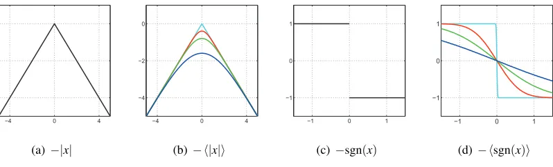
Figure 1: Non-differentiable functions and their Gaussian expectations. Figures (a) and (c) plot the non-differentiable function ψ(x) =−|x| and the non-continuous function ψ(x) =
−sgn(x). Figures (b) and (c) plot the expectations of those functions for Gaussian dis-tributedx as a function of the Gaussian meanm: hψ(x)iN(x|m,σ2). The expectations are
smooth w.r.t. the Gaussian mean. As the variance of the Gaussian tends to zero the ex-pectation converges to the underlying function value. Gaussian exex-pectations taken w.r.t.
N
x|m,σ2whereσ=0.0125,0.5,1,2.3.1 G-KL Bound Differentiability
Whilst the target density of our model may not be differentiable inwthe G-KL bound with respect to the variational momentsm,S frequently is. See Figure 1 for a depiction of this phenomenon for two, simple, non-differentiable functions. The G-KL bound is in fact smooth for potential functions that are neither differentiable nor continuous (for example they have jump discontinuities). In Appendix C we show that the G-KL bound is smooth for potential functions that are piecewise smooth with a finite number of discontinuities, and where the logarithm of each piecewise segment is a quadratic. This class of functions includes the widely used Laplace density amongst others.
3.2 G-KL Bound Concavity
If each site potential{φn}Nn=1is log-concave then the G-KL bound
B
KL(m,S)is jointly concave withrespect to the variational Gaussian meanmandCthe upper triangular Cholesky decomposition of covariance such thatS=CTC. We say that f(x)is log-concave if logf(x)is concave inx.
Since the bound depends on the logarithm of ∏Nn=1φnwithout loss of generality we may take N=1. Ignoring constants with respect tomandC, we can write the G-KL bound as
B
KL(m,C)=c. D∑
d=1
logCdd−
1 2m
T
Σ−1m+µTΣ−1m−1
2trace Σ
−1CCT+logφ(wT
h). (8)
Excludinglogφ(wT
To complete the proof1we need to show thatlogφ(wT
h)is jointly concave inmandC. Log-concavity ofφ(x)is equivalent to the statement that for anyx1,x2∈Rand anyθ∈[0,1]
logφ(θx1+ (1−θ)x2)≥θlogφ(x1) + (1−θ)logφ(x2). (9)
Therefore, to show that
E
(m,C):=logφ(wTh)N(w|m,CTC)is concave it suffices to show for any θ∈[0,1]that
E
(θm1+ (1−θ)m2,θC1+ (1−θ)C2)≥θE
(m1,C1) + (1−θ)E(m2,C2).This can be done by making the substitutionw=θm1+ (1−θ)m2+ (θC1+ (1−θ)C2)Tz, giving
E
(θm1+ (1−θ)m2,θC1+ (1−θ)C2) =Z
N
(z|0,I)×logφ θhT m1+CT1z+ (1−θ)hT m2+CT2zdz. Using concavity of logφ(x) with respect to x and Equation (9) with w1=m1+CT1z and w2= m2+CT2zwe have that
E
(θm1+ (1−θ)m2,θC1+ (1−θ)C2)≥θZ
N
(z|0,I)logφ hT m1+CT
1z
dz
+ (1−θ)
Z
N
(z|0,I)logφ hT m2+CT
2z
dz
=θ
E
(m1,C1) + (1−θ)E
(m2,C2).Thus the G-KL bound is jointly concave in m,C provided all site potentials {φn}Nn=1 are
log-concave.
With consequence to the theoretical convergence rates of gradient based optimisation proce-dures, the bound is also strongly-concave. A function f(x)is strongly-concave if there exists some
c<0 such that for all x, ∇2f(x)cI (Boyd and Vandenberghe, 2004, Section 9.1.2).2 For the
G-KL bound the constantccan be assessed by inspecting the covariance of the Gaussian potential, Σ. If we arrange the set of all G-KL variational parameters as a vector formed by concatenating
mand the non-zero elements of the column’s ofCthen the Hessian oflog
N
(w|µ,Σ)is a block diagonal matrix. Each block of this Hessian is either−Σ−1or its submatrix−Σ−1i:D,i:D, where i=2, . . . ,D. The set of eigenvalues of a block diagonal matrix is the union of the eigenvalues of each of the block matrices’ eigenvalues. Furthermore, the eigenvalues of each submatrix are bounded by the upper and lower eigenvalues of−Σ−1. Therefore∇2
B
KL(m,S)cIwherec is−1 times the smallest eigenvalue of Σ−1. The sum of a strongly-concave function and a concave function is strongly-concave and thus the G-KL bound as a whole is strongly-concave.3.3 Summary
In this section, and in Appendix C, we have provided conditions for which the G-KL bound is strongly concave, smooth, has closed sublevel sets and Lipschitz continuous Hessians. Under these
1. This proof was provided by Michalis K. Titsias and simplifies the original presentation made in (Challis and Barber, 2011).
conditions optimisation of the G-KL bound will have quadratic convergence rates using Newton’s method and super-linear convergence rates using quasi-Newton methods (Nocedal and Wright, 2006; Boyd and Vandenberghe, 2004). For larger problems, where cubic scaling properties aris-ing from the approximate Hessian calculations required by quasi-Newton methods are infeasible, we will use limited memory quasi-Newton methods, nonlinear conjugate gradients or Hessian free Newton methods to optimise the G-KL bound.
Concavity with respect to the G-KL mean is clear and intuitive—for any fixed G-KL covariance the G-KL bound as a function of the mean can be interpreted as a Gaussian blurring of logp(w)— see Figure 1. AsS=ν2I→0thenm∗→wMAPwherem∗is the optimal G-KL mean andwMAPis
the maximum a posteriori (MAP) parameter setting.
Another deterministic Gaussian approximate inference procedure for models of the form of Equation (2) are local variational bounding methods (discussed at further length in Section 5.1.1). For log-concave potentials local variational bounding methods, which optimise a different criterion with a different parameterisation to the G-KL bound, have also been shown to result in a convex optimisation problem (Seeger and Nickisch, 2011b). To the best of our knowledge, local varia-tional bounding and G-KL approximate inference methods are the only known concave variavaria-tional inference procedures for models of the form of Equation (2).
Whilst G-KL bound optimisation and MAP estimation share conditions under which they are concave problems, the G-KL objective is often differentiable when the MAP objective is not. Non-differentiable potentials are used throughout machine learning and statistics. Indeed, the practical utility of such non-differentiable potentials in statistical modelling has driven a lot of research into speeding up algorithms to find the mode of these densities—for example see Schmidt et al. (2007). Despite recent progress these algorithms tend to have slower convergence rates than quasi-Newton methods on smooth, strongly-convex objectives with Lipschitz continuous gradients and Hessians.
One of the significant practical advantages of G-KL approximate inference over MAP estima-tion and the Laplace approximaestima-tion is that the target density is not required to be differentiable. With regards to the complexity of G-KL bound optimisation, whilst an additional cost is incurred over MAP estimation from specifying and optimising the variance of the approximation, a saving is made in the number of times the objective and its gradients need to be computed. Quantifying the net saving (or indeed cost) of G-KL optimisation over MAP estimation is an interesting question reserved for later work.
4. Complexity : G-KL Bound and Gradient Computations
In the previous section we provided conditions for which the G-KL bound is strongly concave and differentiable and so provided conditions for which G-KL bound optimisation using quasi-Newton methods will exhibit super-linear convergence rates. Whilst such convergence rates are highly desirable they do not in themselves guarantee that optimisation is scalable. An important practical consideration is the numerical complexity of the bound and gradient computations required by any gradient ascent optimisation procedure.
Discussing the complexity of G-KL bound and gradient evaluations in full generality is com-plex we therefore restrict ourselves to considering one particularly common case. We consider models where the covariance of the Gaussian potential in Equation (2) is spherical,Σ=ν2I, and each potential function is a site projection,φn(w) =φn(wT
computations for each G-KL covariance parameterisation presented in Section 4.1.3 and a range of parameterisations for the Gaussian potential
N
(w|m,Σ).Note that problems whereΣis not a scaling of the identity can be reparameterised to an equiv-alent problem for which it is. For some problems this reparameterisation can provide significant reductions in complexity. The procedure, the domains for which it is suitable, and the possible computational savings it provides are discussed at further length in Appendix E.
For Cholesky factorisations of covariance, S=CTC, of dimension D the bound and gradi-ent contributions from the log det(S)and trace(S) terms in Equation (7) scaleO(D) andO D2
respectively. Terms in Equation (7) that are a function exclusively of the G-KL mean,m, scale at mostO(D)and are the cheapest to evaluate. The computational bottleneck arises from the projected variational variancess2n=kCThnk2required to compute eachlogφn(wT
hn)term. Computing all such projected variances scalesO ND2.3
A further computational expense is incurred from computing theN one dimensional integrals required to evaluate∑Nn=1logφn(wT
hn). These integrals are computed either numerically or ana-lytically depending on the functional form ofφn. Regardless, this computation scalesO(N),
possi-bly though with a significant prefactor. When numerical integration is required, we note that since
logφn(wThn)
can be expressed ashlogφn(mn+zsn)iN(z|0,1) we can usually assert that the
inte-grand’s significant mass lies forz∈[−5,5]and so that quadrature will yield sufficiently accurate results at modest computational expense. For all the experiments considered here we used fixed width rectangular quadrature and performing these integrals was not the principal bottleneck. For modelling scenarios where this is not the case we note that a two dimensional lookup table can be constructed, at a one off cost, to approximatehlogφ(m+zs)iN(z|0,1)and its derivatives as a function ofmands.
Thus for a broad class of models the G-KL bound and gradient computations scaleO ND2for general parameterisations of the covarianceS=CTC. In many problems of interest the fixed vectors
hn are sparse. LettingL denote the number of non-zero elements in each vector hn, computing
s2n Nn=1 scales nowO(NDL) where frequentlyL≪D. Nevertheless, such scaling for the G-KL method can be prohibitive for large problems and so constrained parameterisations are required.
4.1 Constrained Parameterisations of G-KL Covariance
Unconstrained G-KL approximate inference requires storing and optimising 12D(D+1)parameters to specify the G-KL covariance’s Cholesky factorC. In many settings this can be prohibitive. To this end we now consider constrained parameterisations of covariance that reduce both the time and space complexity of G-KL procedures.
Gaussian densities can be parameterised with respect to the covariance or its inverse the preci-sion matrix. A natural question to ask is which of these is best suited for G-KL bound optimisation. Unfortunately, the G-KL bound is neither concave nor convex with respect to the precision ma-trix. What is more, the complexity of computing the φn site potential contributions to the bound
increases for the precision parameterised G-KL bound. Thus the G-KL bound seems more naturally parameterised in terms of covariance than precision.
3. We note that since a Gaussian potential,N(w|µ,Σ), can be written as a product overDsite projection potentials
4.1.1 OPTIMALG-KL COVARIANCESTRUCTURE
As originally noted by Seeger (1999a), the optimal structure for the G-KL covariance can be as-sessed by calculating the derivative of
B
KL(m,S)with respect toSand equating it to zero. Doing so,SsatisfiesS−1=Σ−1+HΓHT, (10)
whereH= [h1, . . . ,hn]andΓis diagonal such that
Γnn=
z2−1logφn(mn+zsn) 2s2
n
N(z|0,1)
. (11)
Γdepends onSthrough the projected variance termss2n=hTnShnand Equation (10) does not provide a closed form expression to solve forS. Furthermore, iterating Equation (10) is not guaranteed to converge to a fixed point or uniformly increase the bound. Indeed this iterative procedure frequently diverges. We are free, however, to directly optimise the bound by treating the diagonal entries of Γas variational parameters and thus change the number of parameters required to specifySfrom
1
2D(D+1)toN. This procedure, whilst possibly reducing the number of free parameters, requires
us to compute log det(S) whereShas no convenient structure and so in general scalesO D3— infeasible whenD≫1.
A further consequence of using this parameterisation of covariance is that the bound is non-concave. We know from Seeger and Nickisch (2011b) that parameterising Saccording to Equa-tion (10) renders log det(S)concave with respect to(Γnn)−1. However the site projection potentials
are not concave with respect to(Γnn)−1thus the bound is neither concave nor convex for this
param-eterisation resulting in convergence to a possibly local optimum. Non-convexity andO D3scaling motivates the search for better parameterisations of covariance. In Appendix B we provide equa-tions for each term of the G-KL bound and its gradient for each of the covariance parameterisaequa-tions considered below.
4.1.2 FACTORANALYSIS
Parameterisations of the formS=ΘΘT
+diag d2can capture theKleading directions of variance
for aD×K dimensional loading matrixΘ. Unfortunately this parameterisation renders the G-KL bound non-concave. Non-concavity is due to the entropic contribution log det(S) which is not even unimodal. All other terms in the bound remain concave under this factorisation. Provided one is happy to accept convergence to possibly local optima, this is still a useful parameterisation. Computing the projected variances withSin this form scalesO(NDK)and evaluating log det(S)
and its derivative scalesO K2(K+D).
4.1.3 CONSTRAINEDCONCAVEPARAMETERISATIONS
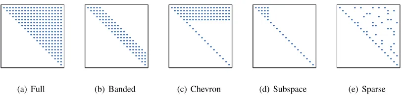
(a) Full (b) Banded (c) Chevron (d) Subspace (e) Sparse
Figure 2: Sparsity structure for constrained concave Cholesky decompositions of covariance.
a marginal independence relation between parameterswi andwj. Conversely, a zero at the(i,j)th
element of precision corresponds to a independence relation between parameterswi andwj when
conditioned on the other remaining parameters.
Banded Cholesky. The simplest option is to constrain the Cholesky matrix to be banded, that isCi j =0 for j>i+BwhereBis the bandwidth. Doing so reduces the cost of a single bound or
gradient computation to O(NDB). Such a parameterisation describes a sparse covariance matrix and assumes zero covariance between variables that are indexed out of bandwidth. The precision matrix for banded Cholesky factorisations of covariance will in general be non-sparse.
Chevron Cholesky. We constrain C such thatCi j =Θi j when j≥i and i≤K, Cii=di for i>Kand 0 otherwise. We refer to this parameterisation as the chevron Cholesky since the sparsity structure has a broad inverted ‘V’ shape—see Figure 2. Generally, this constrained parameterisation results in a non-sparse covariance but sparse precision. This parameterisation is not invariant to index permutations and so not all covariates have the same representational power. For a Cholesky matrix of this form bound and gradient computations scaleO(NDK).
Sparse Cholesky.In general the bound and gradient can be evaluated more efficiently if we im-pose any fixed sparsity structure on the Cholesky matrixC. In certain modelling scenarios we know a priori which variables are marginally dependent and independent and so may be able construct a sparse Cholesky matrix to reflect that domain knowledge. This is of use in cases where a low band width index ordering cannot be found. For a sparse Cholesky matrix withDK non-zero elements bound and gradient computations scaleO(NDK).
Subspace Cholesky. Another reduced parameterisation of covariance can be obtained by consid-ering arbitrary rotations in parameter space,S=ET
CT
CEwhereEis a rotation matrix which forms an orthonormal basis overRD. Substituting this form for the covariance into Equation (8) and for Σ=ν2Iwe obtain, up to a constant,
B
KL(m,C)=c.∑
ilogCii−
1 2ν2
kCk2+kmk2+ 1
ν2µ
T
m+
∑
nhlogφ(mn+zsn)iz
where sn =kCTEThnk. One may reduce the computational burden by decomposing E into two
submatrices such thatE= [E1,E2]whereE1isD×KandE2isD×LforL= (D−K). Constraining Csuch thatC=blkdiag(C1,cIL×L), withC1aK×KCholesky matrix we have that
s2n=kCT1ET1hnk2+c2(khnk2− kET1hnk2),
scaling inKnotD. Further savings can be made if we use banded subspace Cholesky matrices: for
C1having bandwidthBeach bound evaluation and associated gradient computation scalesO(NBK). The success of the subspace Cholesky factorisation depends on how wellE1captures the leading
directions of variance. One simple approach to selectE1is to use the leading principal components
of the ‘data set’H. Another option is iterate between optimising the bound with respect to{m,C1,c}
andE1. We consider two approaches for optimisation with respect toE1. The first uses the form for
the optimal G-KL covariance, Equation (11). By substituting in the projected mean and variance termsmnands2ninto Equation (11) we can setE1to be a rankK approximation to thisS. The best
rankKapproximation is given by evaluating the smallestKeigenvectors ofΣ−1+HΓHT
. For very large sparse problemsD≫1 we approximate this using the iterative Lanczos methods described by Seeger and Nickisch (2010). For smaller non-sparse problems more accurate approximations are available. The second approach is to optimise the G-KL bound directly with respect toE1under the
constraint that the columns ofE1are orthonormal. One route to achieving this is to use a projected
gradient ascent method. Each of these methods and the associated subspace G-KL gradients are presented in greater detail in Appendix B.4.
5. Comparing Gaussian Approximate Inference Procedures
Due to their favourable computational and analytical properties multivariate Gaussian densities are used by many deterministic approximate inference routines. For models of the form of Equa-tion (2) three popular, deterministic, Gaussian, approximate inference techniques are local varia-tional bounding, Laplace approximations, and expectation propagation with an assumed Gaussian density. In this section we briefly review and compare these methods to the G-KL procedure.
Of the three Gaussian approximate inference methods listed above only one, local variational bounding, provides a lower-bound to the normalisation constantZ. In Section 5.1 we give a brief overview of local bounding procedures and show that the G-KL lower-bound dominates the local lower-bound on logZ.
In Section 5.2 we discuss the applicability of each Gaussian approximate inference method. Specifically we describe the computational scaling properties of each of the algorithms and the potential functions to which they can successfully be applied
5.1 Gaussian Lower-Bounds
An attractive property of G-KL approximate inference is that it provides a strict lower-bound on logZ. Lower-bounding procedures are particularly useful for a number of theoretical and practical reasons. The primary theoretical advantage is that it provides concrete exact knowledge aboutZ
and thus also the target density p(w). Lower-bounds may also be used in conjunction with upper bounds to form bounds on marginal quantities of interest (Gibbs and MacKay, 2000). Thus the tighter the lower-bound on logZthe more informative it is. Practically, optimising a lower-bound is often a more numerically stable task than the criteria provided by other deterministic approximate inference methods.
−2 0 2 0
0.5 1
(a)
−5 0 5
0 0.5 1
(b)
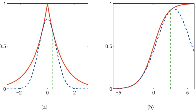
Figure 3: Exponentiated quadratic lower-bounds for two super-Gaussian potential functions: (a) Laplace potential and lower-bound with operating point at 0.5; (b) Logistic sigmoid po-tential and lower-bound with operating point at 2.5.
of local variational bounding procedures. In Section 5.1.2 we prove that G-KL provides a tighter lower-bound onZthan local lower-bounding methods.
5.1.1 LOCALVARIATIONALBOUNDS
Local variational procedures lower-bound Z by replacing each potential φn in Equation (2) with
a function that lower-bounds it and that renders the integral as a whole analytically tractable. Tractability is obtained by using exponentiated quadratic lower-bounds for each non-Gaussian site potential {φn}Nn=1. Local variational bounding procedures that use exponentiated quadratic site
bounds return a Gaussian approximation to the target densityp(w).
Site potentialsφnare known to have tight exponentiated quadratic lower-bounds provided they
are super-Gaussian (Palmer et al., 2006). A function f(x)is said to be super-Gaussian if∃b∈R s.t. forg(x):=logf(x)−bxis even, convex and decreasing as a function ofy=x2. A number of potential functions of significant practical utility are super-Gaussian, examples include: the logistic sigmoidφ(x) = (1+exp(−x))−1, the Laplace densityφ(x)∝exp(−|x|)and the Student’stdensity—
see Figure 3 for plots of these potential functions and their respective lower-bounds.
Each site projection potential function is lower-bounded by an exponentiated quadratic param-eterised inwand a variational parameterξn. Since exponentiated quadratics are closed under
mul-tiplication one may bound the product of site potentials by an exponentiated quadratic also
∏
n
φn(w
T
hn)≥c(ξ)e− 1 2w
T
F(ξ)w+wT
f(ξ), (12)
where the matrixF(ξ), vectorf(ξ)and scalarc(ξ)depend on the specific functions{φn}Nn=1and the
any setting ofwthere exists a setting ofξfor which the bound is tight. Thus we can obtain a bound onZby substituting Equation (12) into Equation (2):
Z=
Z
N
(w|µ,Σ)N
∏
n=1
φn(w
T
hn)dw
≥ Z
N
(w|µ,Σ)c(ξ)e−12wT
F(ξ)w+wT f(ξ)dw
=c(ξ) e− 1 2µ
T
Σ−1µ
p
det(2πΣ)
Z
e−12w
T Aw+wT
bdw, (13)
where
A:=Σ−1+F(ξ) and b:=Σ−1µ+f(ξ). (14) Whilst bothA and bare functions of ξ, we drop this dependency for a more compact notation. One can interpret Equation (13) as a Gaussian approximation to the target density where p(w)≈
N
w|A−1b,A−1. Completing the square in Equation (13) and integrating, we have logZ≥B(ξ), whereB
(ξ) =logc(ξ)−12µ T
Σ−1µ+1 2b
T
A−1b−1
2log det(2πΣ)− 1
2log det(2πA).
To obtain the tightest bound on logZone then maximises
B(ξ)
with respect toξ.5.1.2 COMPARINGG-KLANDLOCALBOUNDS
An important question is which method, local or G-KL, gives a tighter lower-bound on logZ. Each bound derives from a fundamentally different criterion and it is not immediately clear which if either is superior. The G-KL bound has been noted before, empirically in the case of binary classifi-cation (Nickisch and Rasmussen, 2008) and analytically for the special case of symmetric potentials (Seeger, 2009), to be tighter than the local bound. It is tempting to conclude that such observed su-periority of the G-KL method is to be expected since the G-KL bound has potentially unrestricted covarianceSand so a richer parameterisation. However, many problems have more site potentials φnthan Gaussian moment parameters, that isN>12D(D+3), and the local bound in such cases has
a richer parameterisation than the G-KL.
We derive a relation between the local and G-KL bounds for {φn}Nn=1 generic super-Gaussian
site potentials. We first substitute the local bound on ∏Nn=1φn(wThn), Equation (12), into
Equa-tion (4) to obtain a new bound
B
KL(m,S)≥B
˜KL(m,S,ξ),where
2 ˜
B
KL=−2hlogq(w)i −log det(2πΣ) +2 logc(ξ)−D(w−µ)TΣ−1(w−µ)E−wTF(ξ)w+2wTf(ξ).
Using Equation (14) this can be written as
˜
B
KL=−hlogq(w)i −12log det(2πΣ) +logc(ξ)− 1 2µ
T
Σ−1µ−1 2
m
,
S
B
(
m
,
S
)
˜
B
KLm
ξ,
S
ξB
KL(
m
ξ,
S
ξ)
B
(
ξ
) =
B
˜
KL(
m
ξ,
S
ξ,
ξ
)
B
KLm
∗,
S
∗B
KL(
m
∗,
S
∗)
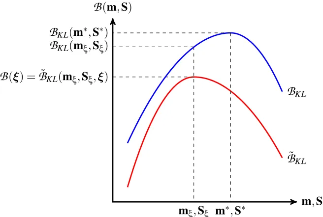
Figure 4: Schematic of the relation between the G-KL bound,
B
KL (blue), and the weakened KL bound, ˜B
KL (red), plotted as a function of the Gaussian moments m and Swith ξ fixed. For any setting of the local site bound parameters ξ we have that
B
KL(m,S) ≥B
˜KL(m,S,ξ). We show in the text that the local bound,B(ξ)
, is the maximum of the weakened KL bound, that is thatB
(ξ) = maxm,SB
˜(m,S,ξ) withmξ,Sξ=argmaxm,S
B(m
˜ ,S,ξ)in the figure. The G-KL bound can be optimised beyondB
KL mξ,Sξ
to obtain different, optimal G-KL momentsm∗andS∗that achieve a tighter lower-bound on logZ.
By defining ˜q(w) =
N
w|A−1b,A−1we obtain˜
B
KL=−KL(q(w)|q˜(w))−12log det(2πΣ) +logc(ξ)− 1 2µ
T Σ−1µ
+1
2b T
A−1b−1
2log det(2πA).
Sincem,Sonly appear viaq(w)in the KL term, the tightest bound is given whenm,Sare set such thatq(w) =q˜(w). At this setting the KL term in ˜
B
KLis zero andmandSare given bySξ= Σ−1+F(ξ)
−1
, mξ=Sξ Σ−1µ+f(ξ)
,
and ˜
B
KL mξ,Sξ,ξ
=
B
(ξ). To reiterate,mξ andSξmaximise ˜B
KL(m,S,ξ) for any fixed settingofξ. Since
B
KL(m,S)≥B
˜KL(m,S,ξ)we have that,The G-KL bound can be optimised beyond this setting and can achieve an even tighter lower-bound on logZ,
B
KL(m∗,S∗) =maxm,S
B
KL(m,S)≥B
KL(mξ,Sξ).Thus optimal G-KL bounds are provably tighter than both the local variational bound and the G-KL bound calculated using the optimal local bound momentsmξandSξ. A graphical depiction of this result is presented in Figure 4.
The experimental results presented in Section 6 show that the improvement in bound values can be significant. Furthermore, constrained parameterisations of covariance, introduced in Sec-tion 4, which are required whenD≫1, are also frequently observed to outperform local variational solutions despite the fact that they are not provably guaranteed to do so.
5.2 Complexity and Model Suitability Comparison
We briefly review the core computational bottlenecks and the conditions placed on the potential functions by the local variational bounding, the Laplace approximation and the Gaussian expecta-tion propagaexpecta-tion approximate inference methods. A more thorough comparison of these techniques in the context of binary Gaussian Process classification can be found in Nickisch and Rasmussen (2008). Subsequently, we go onto summarise and compare these properties versus the G-KL proce-dure.
5.2.1 LAPLACE APPROXIMATIONS
Laplace methods, see Barber (2012) for an introduction, approximate the target density with a Gaussian whose mean is centered at the mode of p(w)and whose covariance is the inverse Hes-sian at the mode of logp(w). The computational complexity of finding the mode is that of a continuous optimisation problem overD real valued parameters on the joint likelihood objective
N
(w|µ,Σ)∏nφn(w). Evaluating the Laplace estimate to logZ requires computing the determi-nant of the Hessian, and so scalesO D3which, importantly, only needs to be computed once. To apply the Laplace approximation we require that the target density be twice continuously differen-tiable, that is we require that each potential function{φn}Nn=1be twice continuously differentiable.Provided the Laplace approximation is valid it is generally the fastest of the methods listed here.
5.2.2 LOCALVARIATIONALBOUNDING
Local variational bounding methods, as detailed in Section 5.1.1, haveNfree variational parameters— one for each site potentialφn. Optimising the bound, using either generalised expectation
maximi-sation or gradient based methods, requires solving N linear symmetric D×Dsystems. Efficient exact implementations of this method maintain the covariance using its Cholesky factorisation and perform efficient rank one Cholesky updates (Seeger, 2007). Doing so each round of updates scales
O ND2. As detailed in Section 5.1.1, local variational bounding procedures are applicable pro-vided tight exponentiated quadratic lower-bounds to the site projection potentials{φn}Nn=1 exist—
that is each site potential is required to be super-Gaussian (Palmer et al., 2006).
Section 5.1.1, and its derivative needs to be computed. Second, these algorithms use approximate methods to evaluate the marginal variances that are required to drive local variational bound opti-misation. Marginal variances are approximated either by constructing low rank factorisations ofA
using iterative Lanczos methods or by perturb and MAP sampling methods (Papandreou and Yuille, 2010; Seeger, 2010; Ko and Seeger, 2012). Both of these approximations can greatly increase the speed of inference and the size of problems to which local procedures can be applied. Unfortunately, these relaxations are not without consequence regarding the quality of approximate inference. For example, the log det(A)term is no longer exactly computed and a lower-bound on logZis no longer maintained—only an estimate of logZ is provided. Lanczos approximated marginal variances are often found to be strongly underestimated and bound values strongly overestimated. Whilst the scaling properties are in general problem and user dependent, roughly speaking, these relaxations reduce the computational complexity to scaling O KD2 whereK is the rank of the approximate covariance factorisation.
5.2.3 GAUSSIANEXPECTATIONPROPAGATION
Gaussian expectation propagation methods seek to approximate the target density by sequentially matching moments between marginals of the variational Gaussian distribution and a density con-structed from the Gaussian approximation and individual site potentials (Minka, 2001). Gaussian expectation propagation (G-EP), for problems of the form of Equation (2), is parameterised us-ing 2N free variational parameters, updating each of which requiresN rank oneD×DCholesky updates and the solution ofNsymmetricD-dimensional linear systems—thus scalingO ND2 as-suming N >D. Importantly, G-EP optimises neither a convex nor concave objective and is not guaranteed to converge. Whilst G-EP does not require the site projection potentials to be either smooth or super-Gaussian, convergence issues can occur if they are multimodal or not log-concave.
Provably convergent double loop extensions to G-EP have been developed—see Opper and Winther (2005) and references therein for details. Typically these methods are slower than vanilla G-EP implementations. However, recent algorithmic developments have yielded significant speed ups over vanilla G-EP whilst maintaining the convergence guarantees (Seeger and Nickisch, 2011a). Importantly, however, these procedures require the exact solution of rankDsymmetric linear sys-tems and thus scaleO D3.
5.2.4 G-KL
G-KL approximate inference methods require that each site projection potential has unbounded support onR. Unlike Laplace procedures G-KL is applicable for models with non-differentiable site potentials. Unlike local variational bounding procedures G-KL does not require the site potentials to be super-Gaussian. In contrast to G-EP, which is known to suffer from convergence issues for non log-concave sites, G-KL procedures optimise a strict lower-bound and convergence is guaranteed for gradient ascent optimisation.
When {φn}Nn=1 are log-concave G-KL bound optimisation is a concave problem and we are
Exact implementations of G-KL approximate inference require storing and optimising over
1
2D(D+3)parameters to specify the Gaussian mean and covariance. Often the number of G-KL
parameters is greater than that for Laplace, G-EP or local variational bounding methods. However, the computations required by G-KL methods scale similarly to these other Gaussian approxima-tion methods. Empirically, as we show in Secapproxima-tion 6, G-KL approximate inference is seen to have comparable convergence speeds to local bounding methods and G-EP.
Importantly, G-KL procedures can be made scalable by using constrained parameterisations of covariance that do not require making a priori factorisation assumptions for the approximate posterior density. Scalable covariance decompositions for G-KL inference maintain a strict lower-bound on logZ whereas approximate local bound optimisers do not. G-EP, being a fixed point procedure, has been shown to be unstable when using low-rank covariance approximations and appears constrained to scaleO ND2(Seeger and Nickisch, 2011a).
6. Applications
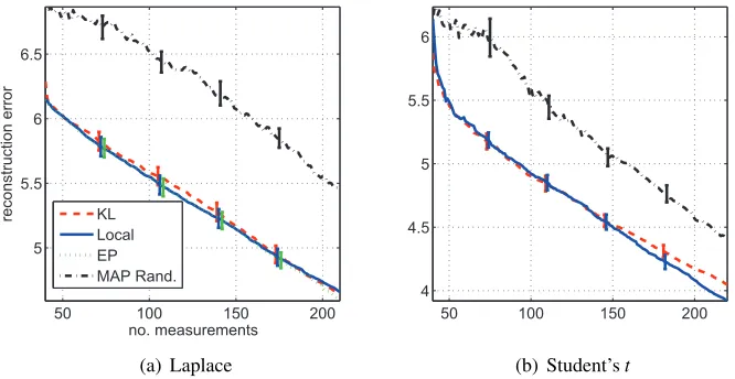
In this section we present results obtained from applying Gaussian KL approximate inference meth-ods to three popular machine learning models. In Section 6.1 we compare deterministic Gaussian approximate inference methods in robust Gaussian process regression models. In Section 6.2 we compare the performance of the constrained parameterisations of G-KL covariance that we pre-sented in Section 4.1.3 in large scale Bayesian logistic regression models. In Section 6.3 we com-pare Gaussian approximate inference methods to drive sequential experimental design procedures in Bayesian sparse linear models.
6.1 Robust Gaussian Process Regression
Gaussian Processes (GP) are a popular non-parametric approach to supervised learning problems, see Rasmussen and Williams (2006) for a thorough introduction, for which inference falls into the general form of Equation (2). Excluding limited special cases, computing Z and evaluating the posterior density, necessary to make predictions and set hyperparameters, is analytically intractable. The supervised learning model for fully observed covariatesX∈RN×Dand corresponding
de-pendent variablesy∈RN is specified by the GP prior on the latent function valuesw∼
N
(µ,Σ) and the likelihoodp(y|w). The GP prior moments are constructed by the GP covariance and mean functions which take the covariatesXand a vector of hyperparametersθas arguments. The posterior on the latent function values,w, is given byp(w|y,X,θ) = 1
Zp(y|w)N(w|µ,Σ).
The likelihood factorises over data instances,p(y|w) =∏Nn=1φ(wn), thus the GP posterior is of the
form of Equation (1) with site projection potentials of the form of Equation (5).
6.1.1 GP REGRESSION
−2 0 2 −2
0 2
(a) Gaussian likelihood
−2 0 2
−2 0 2
(b) Student’stlikelihood
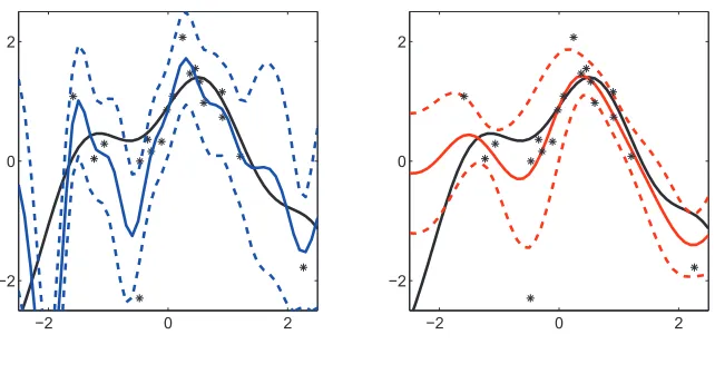
Figure 5: Gaussian process regression with a squared exponential covariance function and (a) a Gaussian or (b) a Student’stlikelihood. Covariance hyperparameters are optimised for a training data set with outliers. Latent function posterior mean (solid) and±1 standard de-viation (dashed) values are plotted in blue (a) and red (b). The data generating function is plotted in black. The Student’stmodel makes more conservative interpolated predictions whilst the Gaussian model appears to over-fit the data.
function rapidly tends to zero for values far from the mean—see Figure 6. Outliers in the training set then do not have to be too extreme to negatively affect test set predictive accuracy. This effect can be especially severe for GP models that have the flexibility to incorporate training set outliers to areas of high likelihood—essentially over-fitting the data.
An example of GP regression applied to a data set with outliers is presented in figure 5(a). In this figure a GP prior with squared exponential covariance function coupled with a Gaussian likelihood over-fits the training data and the resulting predicted values differ significantly from the underlying data generating function.
One approach to prevent over-fitting is to use a likelihood that is robust to outliers. Heavy tailed likelihood densities are robust to outliers in that they do not penalise too heavily observations far from the latent function mean. Two distributions are often used in this context: the Laplace otherwise termed the double exponential, and the Student’s t. The Laplace probability density function can be expressed as
p(y|µ,τ) = 1
2τe−|
y−µ|/τ,
whereτcontrols the variance of the random variableywith var(y) =2τ2. The Student’stprobability
density function can be written as
p(y|µ,ν,σ2) = Γ 1 2(ν+1)
Γ 1 2ν
√
πνσ2 1+
(y−µ)2
νσ2
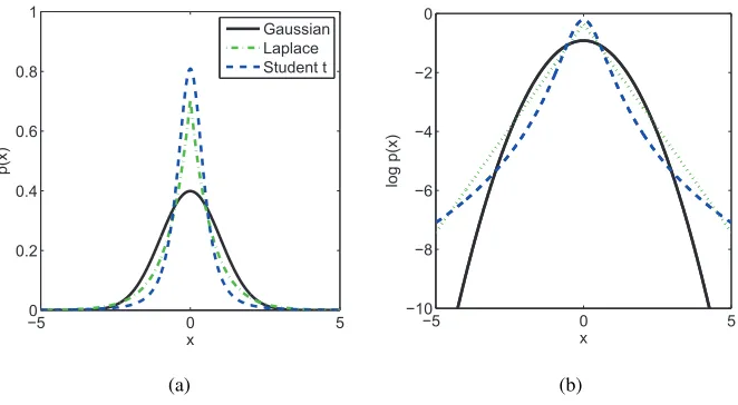
−50 0 5 0.2
0.4 0.6 0.8 1
x
p
(x)
Gaussian Laplace Student t
(a)
−5 0 5
−10 −8 −6 −4 −2 0
x
lo
g
p
(x)
(b)
Figure 6: Gaussian, Laplace and Student’st densities with unit variance: (a) probability density functions and (b) log probability density functions. Laplace and Student’s t densities have stronger peaks and heavier tails than the Gaussian. Student’stwith d.o.f. ν=2.5 and scaleσ2=0.2, Laplace withτ=1/√2.
where ν∈R+ is the degrees of freedom parameter, σ∈R+ the scale parameter, and var(y) = σ2ν/(ν−2) forν>2. As the degrees of freedom parameter becomes increasingly large the
Stu-dent’st distribution converges to the Gaussian distribution. See Figure 6 for a comparison of the Student’st, Laplace and Gaussian density functions.
GP models with outlier robust likelihoods such as the Laplace or the Student’stcan yield signif-icant improvements in test set accuracy versus Gaussian likelihood models (Vanhatalo et al., 2009; Jylanki et al., 2011; Opper and Archambeau, 2009). In figure 5(b) we model the same training data as in figure 5(a) but with a heavy tailed Student’st likelihood, the resulting predictive values are more conservative and lie closer to the true data generating function than for the Gaussian likelihood model.
6.1.2 APPROXIMATEINFERENCE
Whilst Laplace and Student’s t likelihoods can successfully ‘robustify’ GP regression models to outliers they also render inference analytically intractable and approximate methods are required. In this section we compare G-KL approximate inference to other deterministic Gaussian approximate inference methods, namely: the Laplace approximation (Lap), local variational bounding (VB) and Gaussian expectation propagation (G-EP).
Gauss Student’st Laplace
Exact G-KL VB Lap G-KL VB G-EP
C. ST
LML −15±2 −75±2 −240±21 −7±1 8±5 2±2 −−±−− MSE 1.15±0.2 1.6±0.2 23.8±4 2.2±0.4 1.3±1.1 1.2±1.0 −−±−− TLP 0.79±0.10 0.73±0.05 −0.65±0.06 0.41±0.03 0.97±0.06 0.91±0.05 −−±−−
Friedman
LML 70±6 −159±7 −578±34 −97±4 −69±6 −73±8 −−±−− MSE 10±3 5±1 17±2 13±1 5±1 3±1 −−±−− TLP −0.26±0.09 0.12±0.09 −0.54±0.06 −0.65±0.06 0.07±0.09 0.25±0.11 −−±−−
Neal
LML 39±10 −171±14 −962±1 −21±15 −26±9 −27±8 −14±7 MSE 1.7±0.6 2.9±1.1 4.4±1.3 0.9±0.5 0.9±0.4 0.9±0.4 0.9±0.5 TLP 0.22±0.12 0.88±0.03 0.36±0.02 0.67±0.08 0.86±0.04 1.13±0.02 0.91±0.04
Boston
LML 51±3 −133±13 −551±37 −53±3 −60±3 −61±3 −53±4 MSE 26±1 25±2 26±1 23±2 25±2 26±1 22±1 TLP −0.74±0.07 −0.44±0.03 −0.58±0.03 −0.44±0.03 −0.52±0.06 −0.51±0.02 −0.46±0.03
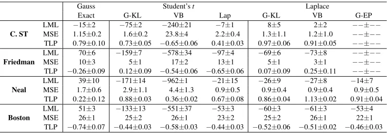
Table 1: Gaussian process regression results for different (approximate) inference procedures, like-lihood models and data sets. First column section: Gaussian likelike-lihood results with exact inference. Second column section: Student’st likelihood results with G-KL, local vari-ational bounding (VB) and Laplace (Lap) approximate inference. Third column section: Laplace likelihood results with G-KL, VB and Gaussian expectation propagation (G-EP) approximate inference. Each row presents the (approximate or lower-bound) log marginal likelihood (LML), test set mean squared error (MSE), or approximate test set log proba-bility (TLP) values obtained by data set. Table values are the mean and standard error of the values obtained over the 10 random partitions of the data.
2011) has alleviated some of G-EP’s convergence issues for Student’s t GP regression, however, these extensions are beyond the scope of this work.
Local variational bounding and G-KL procedures are applied to both likelihood models. For local variational bounding, both the Laplace and Student’stdensities are super-Gaussian and thus tight exponentiated quadratic lower-bounds exist—see Seeger and Nickisch (2010) for the precise forms that are employed in these experiments. Laplace, local variational bounding and G-EP results are obtained using theGPMLtoolbox (Rasmussen and Nickisch, 2010).4 G-KL approximate infer-ence is straightforward, for the G-KL approximate posterior q(w) =
N
(w|m,S) the likelihood’s contribution to the bound ishlogp(y|w)iq(w)=
∑
nD
logφn(mn+z
p
Snn)
E
N(z|0,1).
The equation above is equivalent to Equation (6) withhn=en the unit norm basis vector andφn
the likelihood of thenthdata point. The expectations for the Laplace likelihood site potentials have simple analytic forms—see Appendix B.2.1. The expectations for the Student’st site potentials are evaluated numerically. All other terms in the G-KL bound have simple analytic forms and computations that scale≤O D3. G-KL results are obtained, as for all other results in this paper, using thevgai Matlab package—see Section 8. For the Laplace likelihood model, which is log-concave, Hessian free Newton methods were used to optimise the G-KL bound. For the Student’st
likelihood, which is not log-concave, LBFGS was used to optimise the G-KL bound.
6.1.3 EXPERIMENTALSETUP
We consider GP regression with training data
D
={(yn,xn)}Nn=1 for covariates xn∈RD andde-pendent variablesyn∈R. We assume a zero mean Gaussian process prior on the latent function
values,w= [w1, ...,wN]
T
∼
N
(0,Σ). The covariance,Σ, is constructed as the sum of the squared exponential kernel and the independent white noise kernel,Σmn=k(xm,xn,θ) =σ2see−∑d(xnd−xmd) 2
/ld2+γ2δ(n,m),
wherexnd refers to thedth element of thenthcovariate,σ2seis the ‘signal variance’ hyperparameter, ldthe squared exponential ‘length scale’ hyperparameter, andγthe independent white noise
hyper-parameter (aboveδ(x,y) is the Kronecker delta such thatδ(n,m) =1 ifn=mand 0 otherwise). Covariance hyperparameters are collected in the vectorθ.
We follow the evidence maximisation or maximum likelihood two (ML-II) procedure to es-timate the covariance hyperparameters, that is we set covariance hyperparameters to maximise
p(y|X,θ). Since p(y|X,θ) cannot be evaluated exactly we use the approximated values offered by each of the approximate inference methods. Covariance hyperparameters are optimised numeri-cally using nonlinear conjugate gradients. The marginal likelihood, p(y|X,θ), is not unimodal and we are liable to converge to a local optimum regardless of which inference method is used. All methods were initialised with the same hyperparameter setting. Hyperparameter derivatives for the G-KL bound are presented in Appendix F.2.
Likelihood hyperparameters were selected to maximise the log predicted probability scores on a held out validation data set. Simultaneous likelihood and covariance ML-II hyperparameter opti-misation for the Student’stand Laplace likelihoods yielded poor test set performance regardless of the approximate inference method used (as has been previously reported for Student’stlikelihoods in other experiments (Vanhatalo et al., 2009; Jylanki et al., 2011). For the Student’st likelihood model the d.o.f. parameter was fixed withν=3.
Results were obtained for the four approximate inference procedures on the four data sets using both the Laplace and the Student’st likelihoods. Two UCI data sets were used:5 Boston housing and Concrete Slump Test. And two synthetic data sets: Friedman6 and Neal.7 Each experiment was repeated over 10 randomly assigned training, validation and test set partitions. The size of each data set is as follows: Concrete Slump TestD=9,Ntrn=50,Nval=25,Ntst=28; BostonD=13, Ntrn=100,Nval =100,Ntst=306; Friedman D=10, Ntrn=100,Nval=100, Ntst =100; Neal D=1, Ntrn=100, Nval=100, Ntst =100. Each partition of the data was normalised using the
mean and standard deviation statistics of the training data.
To asses the validity of the Student’stand Laplace likelihoods we also implemented GP regres-sion with a Gaussian likelihood and exact inference.
6.1.4 RESULTS
Results are presented in Table 1. Approximate log marginal likelihood (LML), test set mean squared error (MSE) and approximate test set log probability (TLP) mean and standard error values obtained over the 10 partitions of the data are provided. It is important to stress that the TLP values are approximate values for all methods, obtained by summing the approximate log probability of each
5. UCI data sets can be downloaded fromarchive.ics.uci.edu/ml/datasets/.
test point using the surrogate score presented in Appendix F.1. For G-KL and VB procedures the TLP values are not lower-bounds.
The results confirm the utility of heavy tailed likelihoods for GP regression models. Test set predictive accuracy scores are higher with robust likelihoods and approximate inference methods than with a Gaussian likelihood and exact inference. This is displayed in the lower MSE error and higher TLP scores of the best performing robust likelihood results than for the Gaussian likelihood. Exact inference for the Gaussian likelihood model achieves the greatest LML in all problems except the Concrete Slump Test data. That exact inference with a Gaussian likelihood achieves the strongest LML and weak test set scores implies the ML-II procedure is over-fitting the training data with this likelihood model.
For the Student’s t likelihood the performance of each approximate inference method varied significantly. VB results were uniformly the weakest. We conjecture this is an artifact of the squared exponential local site bounds employed by thegpmltoolbox poorly capturing the non log-concave potential functions mass. For Student’st potentials improved VB performance has been reported by employing bounds that are composed of two terms on disjoint partitions of the domain (Seeger and Nickisch, 2011b), validating their efficacy in the context of Student’stGP regression models is reserved for future work. For the test set metrics G-KL approximate inference achieves the strongest performance.
Broadly, the Laplace likelihood achieved the best results on all data sets. G-EP frequently did not converge for both the Friedman and Concrete Slump Test problems and so results are not pre-sented. Unlike the Student’st likelihood model, results are more consistent across approximate inference methods. G-KL achieves a narrow but consistently superior LML value to VB. Approxi-mate test set predictive values are roughly the same for all inference methods with VB achieving a small advantage.
We reiterate that standard G-EP approximate inference, as implemented in the GPML toolbox, was used to obtain these results. The authors did not anticipate convergence issues for G-EP in the GP models considered—the Laplace likelihood model’s log posterior is concave and the system has full rank. Power G-EP, as proposed in Minka (2004), has previously been shown to have robust convergence for under determined linear models with Laplace potentials (Seeger, 2008). Similarly, we expect that power G-EP would also exhibit robust convergence in GP models with Laplace like-lihoods. Verifying this experimentally and assessing the performance of power G-EP approximate inference in noise robust GP regression models is left for future work.
The G-KL LML uniformly dominates the VB values. This is theoretically guaranteed for a model with fixed hyperparameters and log-concave site potentials, see Section 5.1.2 and Section 3.2. However, the G-KL bound is seen to dominate the local bound even when these conditions are not satisfied. The results show that both G-KL bound optimisation and G-KL hyperparameter opti-misation is numerically stable. G-KL approximate inference appears more robust than G-EP and VB—G-KL hyperparameter optimisation always converged, often to a better local optima.
6.1.5 SUMMARY
likelihood function p(yn|wn). Furthermore, we have seen that G-KL optimisation is numerically
robust, in all the experiments G-KL converged and achieved strong performance.
6.2 Bayesian Logistic Regression
In this section we examine the relative performance, in terms of speed and accuracy of inference, of each of the constrained G-KL covariance decompositions presented in Section 4.1.3. As a bench mark, we also compare G-KL approximate inference results to scalable approximate VB meth-ods with marginal variances approximated using iterative Lanczos methmeth-ods (Seeger and Nickisch, 2011b). Our aim is not make a comparison of deterministic approximate inference methods for Bayesian logistic regression models, see Nickisch and Rasmussen (2008) to that end, but to investi-gate the time accuracy trade-offs of each of the constrained G-KL covariance parameterisations.
Given a data set,
D
={(yn,xn),n=1, . . . ,N}with class labelsyn∈ {−1,1}and covariatesxn∈RD, Bayesian logistic regression models the class conditional distribution using p(y=1|w,x) = σ wTx, withσ(x):=1/(1+e−x)the logistic sigmoid function andw∈RDa vector of parameters. Under a Gaussian prior,
N
(w|0,Σ), the posterior is given byp(w|
D
) = 1Z
N
(w|0,Σ) N∏
n=1
σ ynwTxn. (15)
Where we have used the symmetry property of the logistic sigmoid such that p(y=−1|w,x) =
1−p(y=1|w,x) =σ −wT
x. The expression above is of the form of Equation (2) with log-concave site projection potentialsφn(x) =σ(x)andhn=ynxn.
6.2.1 EXPERIMENTALSETUP
We synthetically generate the data sets. The data generating parameter vectorwtr∈RDis sampled
from a factorising standard normalwtr∼
N
(0,I). The covariates, {xn}Nn=1, are generated by first sampling an independent standard normal, then linearly transforming these vectors to impose corre-lation between some of the dimensions, and finally the data is renormalised so that each dimension has unit variance. The linear transformation matrix we use to impose correlation between covariates is a sparse square matrix generated as the sum of the identity matrix and a sparse matrix with one el-ement from each row sampled from a standard normal. Class labelsyn∈ {1,−1}are sampled fromthe likelihoodp(yn=1|w,xn) =σ(wTxn). The inferential model’s prior and likelihood distributions
are set to match the data generating process.
Results are obtained for a range of data set dimensions: D=250,500,1000 andN=1
2D,D,5D.
We also vary the size of the constrained covariance parameterisations, which is reported asKin the result tables. For chevron CholeskyKrefers to the number of non-diagonal rows ofC. For subspace CholeskyKis the dimensionality of the subspace. For banded CholeskyKrefers to the band width of the parameterisation. For the factor analysis (FA) parameterisationK refers to the number of factor loading vectors. For local variational bounding (VB) approximate inferenceKrefers to the number of Lanczos vectors used to update the variational parameters. The parameterKis varied as a function of the parameter vector dimensionality withK=0.05×DandK=0.1×D.
Ntrn=250 Ntrn=500 Ntrn=2500 K=25 K=50 K=25 K=50 K=25 K=50 Time (s) G-KL
Chev 0.49±0.02 0.69±0.08 1.25±0.04 1.36±0.04 16.50±0.89 17.31±0.82 Band 0.96±0.02 1.37±0.02 2.25±0.10 4.06±0.29 24.31±0.96 29.60±1.18 Sub 0.73±0.01 0.93±0.03 1.41±0.03 1.93±0.04 11.89±0.54 15.26±1.02 FA 2.05±0.26 2.29±0.21 2.92±0.17 3.47±0.17 20.06±1.51 22.69±2.70 VB 0.37±0.00 0.47±0.01 0.46±0.02 0.52±0.00 1.56±0.03 1.85±0.01 ˜
B G-KL
Chev −1.19±0.01 −1.15±0.01 −0.93±0.01 −0.91±0.01 −0.42±0.00 −0.41±0.00 Band −1.15±0.01 −1.09±0.01 −0.92±0.01 −0.88±0.01 −0.42±0.00 −0.41±0.00 Sub −3.08±0.02 −2.20±0.01 −1.90±0.01 −1.46±0.01 −0.62±0.00 −0.54±0.00 FA −1.19±0.01 −1.17±0.01 −0.93±0.01 −0.91±0.01 −0.41±0.00 −0.40±0.00
VB –±– –±– –±– –±– –±– –±–
kw−wtrk2/D G-KL
Chev 0.88±0.00 0.87±0.00 0.84±0.00 0.84±0.00 0.64±0.00 0.64±0.00 Band 0.87±0.00 0.87±0.00 0.84±0.00 0.84±0.00 0.64±0.00 0.64±0.00 Sub 0.88±0.00 0.87±0.01 0.87±0.00 0.86±0.00 0.71±0.00 0.70±0.00 FA 0.88±0.00 0.87±0.01 0.84±0.00 0.84±0.00 0.64±0.00 0.64±0.00 VB 0.90±0.00 0.89±0.00 0.89±0.00 0.88±0.00 0.72±0.00 0.72±0.00 logp(y∗|X∗)/Ntst
G-KL
Chev −0.58±0.01 −0.58±0.01 −0.50±0.01 −0.49±0.01 −0.18±0.00 −0.18±0.00 Band −0.58±0.01 −0.57±0.01 −0.50±0.01 −0.49±0.01 −0.18±0.00 −0.18±0.00 Sub −0.72±0.02 −0.65±0.02 −0.63±0.01 −0.59±0.01 −0.20±0.00 −0.20±0.00 FA −0.58±0.01 −0.58±0.01 −0.51±0.01 −0.50±0.01 −0.18±0.00 −0.18±0.00 VB −0.75±0.02 −0.77±0.02 −0.63±0.01 −0.64±0.01 −0.20±0.00 −0.20±0.00
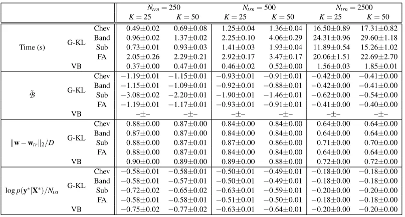
Table 2: Synthetic Bayesian logistic regression results for a model with unit variance Gaussian priorw∼
N
(0,I)with dim(w) =500, likelihood p(y|w,X) =∏Ntrnn=1σ(ynw
T
xn), class la-bels yn∈ {+1,−1} andNtst =5000 test points. G-KL results obtained using chevron
Cholesky (Chev), banded Cholesky (Band), subspace Cholesky (Sub) and factor analysis (FA) constrained parameterisations of covariance. Approximate local variational bound-ing (VB) results are obtained usbound-ing low-rank factorisations of covariance computed usbound-ing iterative Lanczos methods. ParameterK denotes the size of the constrained covariance parameterisation.
and updating the subspace basis vectors E each five times. The subspace vectors were updated using the fixed point iteration with the Lanczos approximation (see Appendix B.4.3 for details). For the FA parameterisation the G-KL bound is not concave so we use LBFGS to perform gradient ascent. All otherminFuncoptions were set to default values.
VB approximate inference is achieved using the glm-ie 1.4 package (Nickisch, 2012). VB inner loop optimisation used nonlinear conjugate gradients with at most 50 iterations. The maximum number of VB outer loop iterations was set to 10. All other VBglm-ieoptimisation settings were set to default values. All results for these experiments were obtained using Matlab 2011a on a Intel E5450 3Ghz machine with 8 cores and 64GB of RAM.
6.2.2 RESULTS
Results forD=500 are presented in Table 2. For reasons of space, results forD=250 andD=1000 are presented in Table 3 and Table 4 in Appendix G. The tables present average and standard error scores obtained from 10 synthetically generated data sets.