Mode-Seeking Clustering and Density Ridge Estimation
via Direct Estimation of Density-Derivative-Ratios
Hiroaki Sasaki [email protected]
Graduate School of Information Science Nara Institute of Science and Technology Nara, Japan
Takafumi Kanamori [email protected]
Department of Mathematical and Computing Science Tokyo Institute of Technology
Tokyo, Japan
Center for Advanced Intelligence Project RIKEN
Tokyo, Japan
Aapo Hyv¨arinen [email protected]
Gatsby Computational Neuroscience Unit University College London
London, United Kingdom Department of Computer Science University of Helsinki
Helsinki, Finland
Canadian Institute for Advanced Research
Gang Niu [email protected]
Graduate School of Frontier Sciences The University of Tokyo
Chiba, Japan
Center for Advanced Intelligence Project RIKEN
Tokyo, Japan
Masashi Sugiyama [email protected]
Center for Advanced Intelligence Project RIKEN
Tokyo, Japan
Graduate School of Frontier Sciences The University of Tokyo
Chiba, Japan
Editor:Miguel ´A. Carreira-Perpi˜n´an
Abstract
Modes and ridges of the probability density function behind observed data are useful geometric features. Mode-seeking clustering assigns cluster labels by associating data samples with the near-est modes, and near-estimation of density ridges enables us to find lower-dimensional structures hidden in data. A key technical challenge both in mode-seeking clustering and density ridge estimation
c
is accurate estimation of the ratios of the first- and second-order density derivatives to the density. A naive approach takes a three-step approach of first estimating the data density, then computing its derivatives, and finally taking their ratios. However, this three-step approach can be unreliable because a good density estimator does not necessarily mean a good density derivative estimator, and division by the estimated density could significantly magnify the estimation error. To cope with these problems, we propose a novel estimator for thedensity-derivative-ratios. The proposed estimator does not involve density estimation, but ratherdirectlyapproximates the ratios of den-sity derivatives of any order. Moreover, we establish a convergence rate of the proposed estimator. Based on the proposed estimator, novel methods both for mode-seeking clustering and density ridge estimation are developed, and the respective convergence rates to the mode and ridge of the underlying density are also established. Finally, we experimentally demonstrate that the developed methods significantly outperform existing methods, particularly for relatively high-dimensional data.
Keywords: Density Derivative, Geometric Feature, Mode-Seeking Clustering, Density Ridge Estimation
1. Introduction
Characterizing the probability density function underlying observed data is a fundamental problem in machine learning. One approach is to consider geometric properties of the density such as modes and ridges. Estimation of such geometric properties is a challenging task, yet offers a variety of applications (Wasserman, 2018).
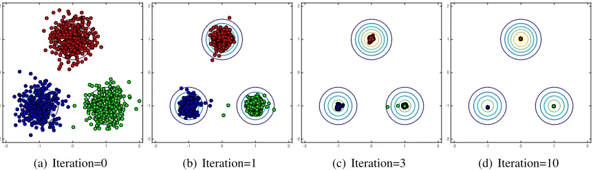
The modes(i.e., local maxima) of probability density functions have received much attention over the years. A motivation of estimating the modes classically appeared in the seminal work on kernel density estimation (Parzen, 1962). More recently, the modes of density functions for random curves have been used in functional data analysis (Gasser et al., 1998). Furthermore, in supervised learning, modal regression associates input variables with the modes of the conditional density function of the output variable, and enables us to simultaneously capture multiple functional rela-tionships between the input and output (Sager and Thisted, 1982; Carreira-Perpi˜n´an, 2000, 2001; Einbeck and Tutz, 2006; Chen et al., 2016a; Sasaki et al., 2016). One of the most natural appli-cations is clustering. Mean shift clustering(MS) makes use of the modes of the estimated density function (Fukunaga and Hostetler, 1975; Cheng, 1995; Comaniciu and Meer, 2002): MS initially re-gards all data samples as candidates for cluster centers, and then iteratively updates them toward the nearest modes of the estimated density by gradient ascent (Fig.1). Finally, the data samples which converge to the same mode are assigned the same cluster label. Unlike standard clustering meth-ods such as k-means clustering (MacQueen, 1967) and mixture-model-based clustering (Melnykov and Maitra, 2010), the notable advantage is that the number of clusters is automatically determined according to the number of detected modes. MS has been applied to a wide range of tasks such as image segmentation (Comaniciu and Meer, 2002; Tao et al., 2007; Wang et al., 2004) and object tracking (Collins, 2003; Comaniciu et al., 2000). (See also a recent review article by Carreira-Perpi˜n´an (2015))
-2 -1 0 1 2 -2
-1 0 1 2
(a) Iteration=0
-2 -1 0 1 2
-2 -1 0 1 2
(b) Iteration=1
-2 -1 0 1 2
-2 -1 0 1 2
(c) Iteration=3
-2 -1 0 1 2
-2 -1 0 1 2
(d) Iteration=10
Figure 1: Illustration of a mode-seeking process. The contour plot indicates the probability density function that generates the data samples.
Figure 2: Examples of the density ridges hidden in data. Gray dot points and green curves indicate data samples and density ridges, respectively.
applications). Density ridge estimation is closely related to manifold estimation. When data is as-sumed to be generated on a lower-dimensional manifold with additive Gaussian noise, density ridge estimation offers a way to circumvent the difficulty of manifold estimation: Genovese et al. (2014) theoretically proved that the density ridges capture the essential properties of such manifolds and es-timating the density ridge is substantially easier than eses-timating the manifold. A practical algorithm calledsubspace constrained mean shift(SCMS) by Ozertem and Erdogmus (2011). SCMS is an extension to MS, but a projected gradient ascent method is performed to find density ridges instead of the gradient ascent method in MS; the gradient vector of the estimated density is projected to the subspace which is orthogonal to the ridge. Such a subspace can be obtained by applying principal component analysis to an estimate of the Hessian matrix of the log-density, which is composed of the ratios of the first- and second-order density derivatives to the density. Along the projected gra-dient vector, SCMS updates data points toward the ridge of the estimated density until convergence. For MS, the technical challenge is accurate estimation of the derivatives of the probability den-sity function. To derive practical methods, MS takes a two-step approach, firstly estimating the probability density function and then computing its derivatives (Comaniciu and Meer, 2002, Sec-tion 2).1 However, this approach can be unreliable because a good density estimator does not
necessarily imply a good density derivative estimator in many practical situations. For example, small random fluctuations in a density estimate can create fake modes and may produce large errors in density-derivative estimation, even if the density estimate is fairly good in terms of density esti-mation (Genovese et al., 2016, Fig.1). Therefore, testing methods have been proposed to investigate whether the estimated modes are real modes from the underlying data density or fake modes due to the random fluctuations (Godtliebsen et al., 2002; Duong et al., 2008; Genovese et al., 2016). For SCMS, it is even more challenging to estimate the ratios of density derivatives to the density, but SCMS also naively estimates the ratios by adding one more step to the two-step approach in MS: the computed density derivatives are divided by the estimated density. However, such a division could strongly magnify estimation error.
To cope with these problems, we propose a novel estimator of the ratios of density derivatives to the density. In stark contrast with the approaches in MS and SCMS, the key idea is todirectly
estimate the ratios without going through density estimation. Moreover, we theoretically analyze the proposed estimator and establish a convergence rate. The direct approach has been adopted and proved to be useful both empirically and theoretically when estimating the ratio of two proba-bility density functions (Sugiyama et al., 2008; Nguyen et al., 2008; Kanamori et al., 2009, 2012; Sugiyama et al., 2012; Kpotufe, 2017). Here, we follow the direct approach in the context of a different problem and derive an estimator in a substantially different way. Previously, a direct es-timator has been proposed for the log-density derivatives (Beran, 1976; Cox, 1985), which are the ratios of first-order density derivatives to the density. On the other hand, the proposed estimator in this paper approximates the ratio of the derivatives of any order to the density, and thus generalizes the previous estimator.
The proposed estimator is first applied to mode-seeking clustering. We derive an update rule for mode-seeking based on a fixed-point algorithm, while inheriting the advantage of MS: the proposed clustering method also does not require the number of clusters to be specified in advance. This is advantageous because clustering is an unsupervised learning problem and tuning the number of clusters is not straightforward in general. Next, based on the mode-seeking clustering, we propose a novel method for density ridge estimation. For both methods, we prove the consistency of the mode and ridge estimators, and establish the convergence rates. Finally, we experimentally demonstrate that our proposed methods outperform MS and SCMS, particularly for high(er)-dimensional data.
2. Direct Estimation of Density-Derivative-Ratios
This section proposes a novel estimator of the ratios of density derivatives to the density and per-forms theoretical analysis.
2.1 Problem Formulation
Suppose thatni.i.d. samples, which were drawn from a probability distribution onRD with density p(x), are available:
D:={xi = (x(1)i , x
(2)
i , . . . , x
(D)
i ) >}n
i=1
i.i.d.
∼ p(x).
Here, our goal is to estimate the ratio of the |j|-th order partial derivative ofp(x) to p(x) from
D={xi}ni=1,
∂jp(x)
p(x) , (1)
where∂j = ∂
|j|
∂j1x(1)∂j2x(2)...∂jDx(D),j = (j1, j2, . . . , jD)
>and|j|= j
1+j2+· · ·+jD for
non-negative integersji = 0,1, . . . ,|j|. For instance, when |j| = 1(or |j| = 2),∂jp(x)/p(x) is a
single element of∇p(x)/p(x)(or of∇∇p(x)/p(x)).
2.2 Least-Squares Density-Derivative-Ratios
Our main idea is to directly fit a modelrj(x)to∂jp(x)/p(x)under the squared-loss:
Jj(rj) :=
Z
rj(x)−
∂jp(x)
p(x)
2
p(x)dx
=
Z
{rj(x)}2p(x)dx−2
Z
rj(x)∂jp(x)dx+
Z
∂jp(x)
p(x)
2
p(x)dx. (2)
The first term on the right-hand side of (2) can be naively estimated from samples and the third term is ignorable, but it seems challenging to estimate the second term because it includes the derivative of the unknown density. However, as in Sasaki et al. (2015), repeatedly applying integration by partsallows us to transform the second term as
Z
rj(x){∂jp(x)}dx= (−1)|j|
Z
{∂jrj(x)}p(x)dx, (3)
where we assumed that as|x(j)| → ∞ for allj, the product of∂
j1rj(x) and∂j2p(x)approaches
zero for any pairs ofj1andj2satisfying|j1|+|j2|=|j| −1for|j1|,|j2|= 0,1, . . . ,|j| −1. As a
result, the right-hand side of (3) can be easily estimated from samples. Then, an empirical version of (2) is given by
b
Jj(rj) :=
1
n
n
X
i=1
n
rj(xi)2−2(−1)|j|∂jrj(xi)
o
After adding the regularizerR(rj), the estimator is defined as the minimizer of
b
rj := argmin
rj
h
b
Jj(rj) +λjR(rj)
i
, (5)
whereλjis the regularization parameter.
We call this method the least-squares density-derivative ratios (LSDDR). Note that when
|j|= 1,Jjis called the Fisher divergence and has been used for parameter estimation of
unnnormal-ized statistical models (Hyv¨arinen, 2005), density estimation with the computationally intractable partition function (Sriperumbudur et al., 2017), and direct estimation of log-density derivatives (Be-ran, 1976; Cox, 1985; Sasaki et al., 2014). Therefore, LSDDR can be regarded as a generalization of such methods to higher-order derivatives.
2.3 Theoretical Analysis of LSDDR
Next, we theoretically analyze LSDDR.
2.3.1 PRELIMINARIES ANDNOTATIONS
For aD-dimensional vectorx∈RD, the norm is defined bykxk:=qPD
j=1(x(j))2. For a domain X(⊆ RD),C(X)denotes the space of all continuous functions onX. Furthermore, we define the
Lp space of functionsf onX: For1 ≤ p ≤ ∞, Lp(X) := {f : kfk
p < ∞}where k · kp is
theLpnorm defined bykfkp :=
R
|f(x)|pdxp1
with the Lebesgue measure for1≤p < ∞and
kfk∞:= ess supx∈X|f(x)|. Forf ∈L1(RD), theFourier transformis defined as
f∧(ω) := 1 (2π)D/2
Z
f(x)e−iω>xdx,
whereidenotes the imaginary unit.
Let H be a reproducing kernel Hilbert space (RKHS) over X uniquely associated with the reproducing kernel k : X × X → R. The norm and inner product on H are denoted byk · kH
andh·,·iH, respectively. k is a real-valued, symmetric and positive definite function and has the
reproducing property: For allx∈ X andf ∈ H,hf, k(·,x)iH=f(x). An example of reproducing
kernels is the Gaussian kernel, k(x,y) = exp
−kx2−σy2k2
whereσ > 0 is the width parameter.
Another example is theMat´ern kernel,k(x,y) =ψ(x−y) = 2Γ(1−s)skx−yks−D/2K
D/2−s(kx−yk),
whose corresponding RKHSHcoincides with the Sobolev spaceH2swith the smoothness parameter s > D/2(Wendland, 2004, Chapter 10):
H=H2s:=
f ∈L2(RD)∩C(RD) :
Z
(1 +kωk2)s|f∧(ω)|2dω<∞
.
Γ(·)denotes the Gamma function, andKv(·)is the modified Bessel function of the second kind of
2.3.2 THECONVERGENCERATE OFLSDDR
Here, we derive a rate of convergence for LSDDR under the RKHS norm. To this end, we assume that the true density-derivative-ratio is contained inH:
r∗j(x) := ∂jp(x)
p(x) ∈ H.
Furthermore, we restrict the search space ofrj toHand express LSDDR withR(rj) =krjk2Has
b
rj = argmin
rj∈H
h
b
Jj(rj) +λjkrjk2H
i
. (6)
To establish a convergence rate under the RKHS norm, we make the following assumptions as in Sriperumbudur et al. (2013):
(A) X is compact.
(B) kis2|j|continuously differentiable.
(C) The following equation holds:
Z
X
k(·,x)∂jp(x)dx= (−1)|j|
Z
X
∂jk(·,x)p(x)dx.
(D) For allj, there exists≥1subject to
Z
X
kk(·,x)k2Hp(x)dx
1
2
<∞ and
Z
X
k∂jk(·,x)kHp(x)dx
1
<∞.
Assumption(A)makesHseparable (Steinwart and Christmann, 2008, Lemma 4.33) and the sepa-rability ofHis required to apply Proposition A.2 in Sriperumbudur et al. (2013). Assumption(B)
ensures that arbitrary functions inHare2|j|continuously differentiable (Steinwart and Christmann, 2008, Corollary 4.36). Assumption(C)holds under mild assumptions ofkandpas in (3). From As-sumption(D),Jj(rj) <∞when= 1. Then, the following theorem establishes the convergence
rate under the RKHS norm:
Theorem 1 Let
C :=
Z
X
k(·,x)⊗k(·,x)p(x)dx,
where⊗denotes the tensor product, be an operator onH. If there existsγ >0such thatrj∗ is in the range ofCγ(i.e.,rj∗ ∈ R(Cγ)), then
kbrj−r∗jkH=OP
n−min
n 1 4,
γ
2(γ+1)
o
,
with= 2andλj =O
n−max
n 1 4,
1 2(γ+1)
o
The proof is given in Appendix A. We followed the proof techniques in Sriperumbudur et al. (2013), but adopted them to a different problem: Sriperumbudur et al. (2013) proposed and analyzed a non-parametric estimator for log-densities with the intractable partition functions based on the Fisher divergence, which is a special case ofJj at|j|= 1. The range space assumptionrj∗ ∈ R(Cγ)is
closely related to the smoothness ofr∗j (Sriperumbudur et al., 2013, Section 4.2): Largerγ implies thatrj∗ is smoother. As seen in Sections 3.3.3 and 4.3.2, Theorem 1 is particularly useful in the analysis of our mode-seeking clustering and density ridge estimation methods.
Remark 2 By following Sriperumbudur et al. (2017, Section 4.2), Theorem 1 has some connection to the minimax theory (Tsybakov, 2009) under Sobolev spaces where for any α > s ≥ 0, the minimax rate is given by
inf
b
rj,n
sup rj∗∈Hα
2
kbrj,n−rj∗kHs
2 n
− α−s
2(α−s)+D.
inf is taken over possible estimators brj,n, andan bnmeans that an/bn has lower- and upper-bounds away from zero and infinity, respectively. To establish a connection to Sobolev spaces, suppose that the Mat´ern kernel is employed whose corresponding RKHS is a Sobolev spaceH =
Hs
2 with the smoothness parameter s > D/2. As proved in Appendix B, when the true density
belongs toL1(RD)(i.e., p ∈ L1(RD)),r∗j ∈ R(Cγ)forγ ≥ 1implies thatrj∗ ∈ H
3D
2 −
1 2+
2 for
arbitrarily small >0. Then, the convergence raten−14 is minimax optimal underH=HD− 1 2+
2 .
Furthermore, this result implies that the dimension effect is veiled through the relative smoothness
between two Sobolev spaces (H
3D
2 −
1 2+
2 and H
D−1 2+
2 ), and therefore the rate in Theorem 1 is
independent of data dimensionD. Details are provided in Appendix B.
2.4 Practical Implementation of LSDDR
Here, we describe practical implementation of LSDDR.
• A practical version of LSDDR: The representer theorem (Zhou, 2008, Theorem 2) states that the estimatorbrj should take the following form:
b
rj(x) =
n
X
i=1
αj(i)k(x,xi) +βj(i)∂j0k(x,x0)
x0=x
i
=
2n
X
i=1
θ(ji)ψ(ji)(x) =θ>jψj(x), (7)
where∂j0 denotes the partial derivative with respect tox0,
θ(ji) :=
(
αj(i) i= 1, . . . , n,
βj(i−n) i=n+ 1, . . . ,2n, ψ
(i)
j (x) :=
(
k(x,xi) i= 1, . . . , n,
∂j0k(x,x0)
x0=x
i−n
i=n+ 1, . . . ,2n.
To estimate θj, we substitute (7) into Jbj in (4). Then, when R(rj) = θj>θj, the optimal
solution ofθjcan be computed analytically as
b
θj := argmin θj
h
θj>Gbjθj−2(−1)|j|θj>hbj+λjθ>jθj i
= (−1)|j|Gbj+λjI2n
−1
b
whereI2ndenotes the2nby2nidentity matrix,
b
Gj :=
1
n
n
X
i=1
ψj(xi)ψj(xi)> and bhj :=
1
n
n
X
i=1
∂jψj(xi).
Finally, a practical version of LSDDR is given by
b
rj(x) :=θbj>ψj(x) =
n
X
i=1
b
α(ji)k(x,xi) +βb
(i)
j ∂
0
jk(x,x
0 )
x0=x
i .
• Model selection by cross-validation: Model selection is a crucial problem in LSDDR. As in standard model selection methods for kernel density estimation (Bowman, 1984; Sheather, 2004), we take a least-squares approach based on (2), and optimize the model parameters (parameters ink(·,·)and the regularization parameterλj) by cross-validation as follows:
1. Divide the samplesD={xi}ni=1 intoT disjoint subsets{Dt}Tt=1.
2. Obtain the estimator br(jt)(x) from D \ Dt (i.e., Dwithout Dt), and then compute Jbj
from the hold-out samples as
CV(t) := 1
|Dt|
X
x∈Dt
n
b
r(jt)(x)
o2
−2(−1)|j|∂jbr
(t)
j (x)
,
where|Dt|denotes the number of elements inDt.
3. Choose the model that minimizes T1 PT
t=1CV(t).
2.5 Notation
In the rest of this paper, we consider LSDDR only for|j|= 1and|j|= 2. Therefore, we use more specific notations as follows:
• (Sections 3 and 4) For|j|= 1, a first order density-derivative-ratio corresponds to a first order derivative of the log-density, and we express the true derivative as
gj(x) :=
∂jp(x)
p(x) =∂jlogp(x),
where∂j := ∂x∂(j). Then, LSDDR togj(x)is denoted by
b
gj(x) :=
2n
X
i=1
b
θ(ji)ψ(ji)(x) = n
X
i=1
b
α(ji)k(x,xi) +βb
(i)
j ∂ 0
jk(x,x0)
x0=x
i ,
where ∂j0 denotes the partial derivative with respect to the j-th coordinate in x0, and the subscriptjofθb
(i)
j is simplified fromjbecause only one element injis one and the others are
zeros when|j|= 1.
• (Section 4) For |j| = 2, we express a true second order density-derivative-ratio by
[H(x)]ij := ∂i∂p(jpx()x) where [H(x)]ij denotes the (i, j)-th element of the matrix H(x).
3. Application to Mode-Seeking Clustering
This section applies LSDDR to mode-seeking clustering.
3.1 Problem Formulation for Clustering
Suppose that we are given a collection of data samples D = {xi}ni=1. The goal of clustering is
to assign a cluster labelci ∈ {1, . . . , c} to each data sample xi, wherec denotes the number of
clusters, and isunknown.
3.2 Brief Review of Mean Shift Clustering
Mean shift clustering (MS) (Fukunaga and Hostetler, 1975; Cheng, 1995; Comaniciu and Meer, 2002) is a popular clustering method, and has been applied in a wide-range of fields such as im-age segmentation (Comaniciu and Meer, 2002; Tao et al., 2007; Wang et al., 2004) and object tracking (Collins, 2003; Comaniciu et al., 2000) (see a recent review article by Carreira-Perpi˜n´an (2015)). MS initially regards all data samples as candidates of cluster centers, and updates them toward the nearest modes of the estimated density by gradient ascent. Finally, the same cluster la-bel is assigned to the data samples which converge to the same mode. Unlike standard clustering methods such ask-means clustering(MacQueen, 1967), MS automatically determines the number of clusters according to the number of detected modes.
To update data samples, the technical challenge is to accurately estimate the gradient ofp(x). MS takes a two-step approach: The first step performs kernel density estimation (KDE) as
b
pKDE(x) :=
1
Zn,h n
X
i=1
KKDE
kx−xik2 2h2
!
,
where KKDE is a kernel function for KDE, Zn,h is the normalizing constant, andh denotes the
bandwidth parameter. Then, the second step computes the partial derivatives ofpbKDE(x)as
∂jbpKDE(x) =
1
h2Z
n,h n
X
i=1
(x(ij)−x(j))GKDE
kx−xik2 2h2
!
= 1
h2Z
n,h
( n
X
i=1
GKDE
kx−xik2 2h2
!)
Pn
i=1x (j)
i GKDE
kx−x
ik2
2h2
Pn
i=1GKDE
k
x−xik2
2h2
−x
(j)
,
whereGKDE(t) =−ddtKKDE(t).
By denoting theτ-th update of a data sample byzkτ = (z(kτ,1), zk(τ,2), . . . , z(kτ,D))>wherezk0 =
xk, setting∂jpbKDE(x) = 0yields the following fixed-point iteration formula:
zk(τ+1,j) =
Pn
i=1x (j)
i GKDE
kzτ k−xik
2
2h2
Pn
i=1GKDE
kzτ k−xik
2
2h2
Simple calculation shows that (8) can be equivalently expressed as
zτk+1 =zkτ+ h
2Z
n,h
Pn
i=1GKDE
kzkτ−xik
2
2h2
∇pbKDE(x)|x=zkτ =z
τ
k+cmKDE(z
τ
k), (9)
where ∇ denotes the vector differential operator with respect to x, and cmKDE(z) =
(mb(1)KDE(z),mb(2)KDE(z), . . . ,mb(KDED) (z))>is called themean shift vectorand defined by
c
mKDE(z) =
h2Zn,h
Pn
i=1GKDE
kz−x
ik2
2h2
∇pbKDE(x)|x=z. (10)
Eq.(9) indicates that MS performs gradient ascent. To speed up MS, acceleration strategies were also developed in Carreira-Perpi˜n´an (2006).
Properties of MS have been theoretically well-investigated (Cheng, 1995; Fashing and Tomasi, 2005; Ghassabeh, 2013; Arias-Castro et al., 2016). For instance, a sequence{zτk, τ = 0,1,2, . . .}
generated by MS converges to a mode ofpbKDE(x)asτ goes infinity (Comaniciu and Meer, 2002;
Li et al., 2007; Ghassabeh, 2013); Carreira-Perpi˜n´an (2007) showed that the algorithm of MS is equivalent to the EM algorithm (Dempster et al., 1977) whenKKDE(t) = exp(−t); Furthermore,
Fashing and Tomasi (2005) proved that MS performs a bound optimization. Although MS has good theoretical properties, the two-step approach in gradient estimation seems practically inappropriate because a good-density estimator does not necessarily mean a good-density gradient estimator. A more appropriate way would be to directly estimate the gradient. Following this idea, we apply LSDDR to mode-seeking clustering.
3.3 Least-Squares Log-Density Gradient Clustering
Here, LSDDR is employed to develop a novel mode-seeking clustering method because LSDDR is an estimator of a single element in the log-density gradient when|j|= 1. The proposed clustering method is called theleast-squares log-density gradient clustering(LSLDGC).
3.3.1 FIXED-POINTITERATION
First, when we estimate thej-th element ing(x) = ∇logp(x), the form of the kernel function is restricted as
k(x,xi) =φ
kx−xik2 2σ2
j
!
,
whereσj denotes a bandwidth parameter, andφis a non-negative, monotonically non-increasing,
convex and differentiable function. For example, whenφ(t) = exp(−t),k(x,xi) is the Gaussian
kernel. Under the restriction, LSDDR can be rewritten as
b
gj(x) = n
X
i=1
"
b
αj(i)φ kx−xik
2
2σ2j
!
+βe
(i)
j
x(ij)−x(j) σj2 ϕ
kx−xik2 2σj2
!#
, (11)
whereβe
(i)
j =−βb
(i)
For our mode-seeking clustering method, we derive a fixed-point iteration similarly to MS.
WhenPn
i=1βe
(i)
j ϕ
kx−xik2
2σ2
j
6
= 0, (11) can be expanded as
b
gj(x) = n
X
i=1
"
b
α(ji)φ kx−xik
2
2σj2
!
+βe
(i)
j x
(j)
i
σj2 ϕ
kx−xik2 2σ2j
!#
−x
(j)
σ2j
n
X
i=1
e
βj(i)ϕ kx−xik
2
σ2j
! = 1 σ2 j n X i=1 e
βj(i)ϕ kx−xik
2
2σ2
j ! Pn i=1
σj2αb(ji)φ
kx−xik2
2σ2
j
+βe
(i)
j x
(j)
i ϕ
kx−xik2
2σ2
j
Pn
i=1βe
(i)
j ϕ
kx−xik2
2σ2
j
−x
(j)
.
As in MS, settingbgj(x) = 0yields the following update formula:
z(kτ+1,j)=
Pn
i=1
σ2
jαb
(i)
j φ
kzτ k−xik
2
2σ2
j
+βe
(i)
j x
(j)
i ϕ
kzτ k−xik
2
2σ2
j
Pn
i=1βe
(i)
j ϕ
kzτ k−xik2
2σ2
j
, (12)
wherezkτdenotes theτ-th update of a data sample initialized byxk. Eq.(12) can be also equivalently
expressed as
z(τ+1,j)=z(τ,j)+ σ
2
j
Pn
i=1βej(i)ϕ
kzτ−x ik2
2σ2
j
bgj(z
τ) =z(τ,j)+
b
m(j)(zτ), (13)
where
b
m(j)(z) := σ
2
j
Pn
i=1βe
(i)
j ϕ
kz−xik2
2σ2
j
bgj(z). (14)
Whenαb
(i)
j = 0andβe
(i)
j = 1/n, (12) is reduced to the MS update formula (8). Thus, LSLDGC
includes MS as a special case.
The form of (12) motivates us to develop a coordinate-wise update rule. Fromj= 1toj=D, we iteratively update one coordinate at a time by simply modifying (12) as
z(kτ+1,j)=
Pn
i=1
σ2jαb(ji)φ
kz˜τ k−xik2
2σ2
j
+βe
(i)
j x
(j)
i ϕ
kz˜τ k−xik2
2σ2
j
Pn
i=1βe
(i)
j ϕ
kz˜τ k−xik2
2σ2
j
, (15)
where
˜
zkτ = (zk(τ+1,1), . . . , zk(τ+1,j−1), zk(τ,j), zk(τ,j+1), . . . , zk(τ,D))>.
3.3.2 SUFFICIENTCONDITIONS FORMONOTONICHILL-CLIMBING
LSLDGC updates data samples towards the modes like hill-climbing. Here, we show sufficient conditions for monotonic hill-climbing, i.e., LSLDGC makes data samples never climbing-down. The challenge in this analysis is that unlike MS, we cannot know the estimated density, and thus it is not straightforward to investigate this property for LSLDGC. To overcome this challenge, we employpath integral2 (Strang, 1991): For the vector fieldg(x) =∇logp(x)and a differentiable curveγ(t), t∈[0, s]connectingxandy, i.e.,γ(0) = y,γ(s) =x, the standard formula of path integral is given by
Dg[x|y] :=
Z s
0
ı<g(γ(t)),γ˙(t)>dt= logp(x)−logp(y), (16)
whereγ˙(t) = ddtγ(t)andı<·,·>denotes the inner product. The notable property of path integral is that the integral is independent of any choice of a path, and determined only by the two points, yandx, as shown in the most right-hand side of (16). In this analysis, we use the following path along with one coordinate at a time repeatedly:
y= (y(1), y(2), y(3), . . . , y(D))→(x(1), y(2), y(3), . . . , y(D))→(x(1), x(2), y(3), . . . , y(D))
→(x(1), x(2), x(3), . . . , y(D))→ · · · →(x(1), x(2), x(3), . . . , x(D)) =x. (17)
By substituting our gradient estimategb(x)into the middle part of (16) under the path (17),
b
D
b
g[x|y] :=
Z s
0
ı<gb(γ(t)),γ˙(t)>dt= D
X
j=1
Z x(j)
y(j) b
gj(x(1), x(2), . . . , z(j), . . . , y(D))dz(j).
(18)
From (16),Db b
g[x|y]can be regarded as an estimator oflogp(x)−logp(y)when we fix the curve
that connectsxandy. Thus,Db b
g[zτk+1|zkτ]≥0for allτ implies that the data samples updated by
LSLDGC never climb down. The following theorem provides some sufficient conditions:
Theorem 3 Suppose thatφis a non-negative, monotonically non-increasing, convex and differen-tiable function. Then, ifαb(ji) = 0andβe
(i)
j ≥ 0, under the coordinate-wise update rule(15)and path(17),
b
D
b
g[zτk+1|z τ k]≥0.
The proof is deferred to Appendix C.
Remark 4 Theorem 3 shows sufficient conditions that LSLDGC with the coordinate-wise update rule(15)makes data samples monotonically hill-climb towards the modes. However, without satis-fying the conditions, we empirically observed that most of data samples monotonically converge to modes. Therefore, we conjecture that some milder conditions exist, and do not apply all sufficient conditions in practice. Practical implementation is described in Section 3.4.
Remark 5 For another update rule(12), sufficient conditions for monotonic hill-climbing were not established as in Theorem 3. However, Theorem 7 implies that accurate mode-seeking is possible for both update rules as long asDb
b
g[zkτ+1|zτk]is kept non-negative for allτ. Therefore, in practice, wheneverDb
b
g[zkτ+1|zτk]is negative, we perform standard gradient ascent. The details are given in Section 3.4.
Remark 6 Sufficient conditions for monotonic hill-climbing have been established in MS (Comani-ciu and Meer, 2002; Li et al., 2007; Ghassabeh, 2013). The main difference is that we obtain the difference of two log-density estimates from a gradient estimate, while previous work directly begins with density estimation based on KDE. Thus, the proof is substantially different.
Theorem 3 holds under the path (17). However, the following theorem states that asnincreases,
b
D
b
g[x|y]approachesDg[x|y], which is independent of the choice of a path:
Theorem 7 Suppose that bothgandgbare finite on the path(17)and the assumptions in Theorem 1 hold. Then, for arbitraryxandy,
Dg[x|y]−Dbgb[x|y]
≤ kg−gbk∞kx−yk1≤OP
n−min
n 1 4,
γ
2(γ+1)
o
,
wherek · k1denotes the`1norm.
The proof is given in Appendix D.
Remark 8 Theorem 7 shows
|Dg[zτk|zτk+1]−Db b
g[zkτ|zkτ+1]| ≤ kg−bgk∞kz
τ
k−zτk+1k1. (19) From(19), the non-negativity ofDb
b
g[zτk|z τ+1
k ]implies thatDg[z τ k|z
τ+1
k ]is also non-negative when
n is sufficiently large. Thus, Theorem 7 ensures that accurate mode-seeking is possible by both update rules(12)and(15).
3.3.3 THECONVERGENCERATE TO THETRUEMODESET
First, we define the set of the true mode points as
M:={µ : g(µ) =0,∇g(µ)≺O}, (20)
where∇g(µ)is the Hessian matrix of the log-density at a mode pointµ, and∇g(µ)≺Omeans that∇g(µ) is (strictly) negative definite. The set of the estimated mode points is also denoted by
c
M. Our goal is to establish the convergence rate betweenMandMcunder the Hausdorff distance:
Haus(A,B) := max sup
x∈A inf
y∈Bkx−yk,ysup∈Bxinf∈Akx−yk
!
, (21)
whereAandBdenote two sets.
Theorem 9 Suppose that the assumptions in Theorem 1 hold. Further assume that each mode point
µ∈ Mis approximated by a unique estimated mode pointµb∈Mc. Then, with high probability,
Haus(Mc,M) =OP
n−min
n 1 4,
γ
2(γ+1)
o
. (22)
The proof can be seen in Appendix E.
Remark 10 Chen et al. (2016b, Theorem 1) established the following convergence rate based on KDE: With the asymptotically optimal bandwidthh=O
n−D1+6
,
Haus(McKDE,M) =OP
n−D2+6
, (23)
where McKDE denotes the set of mode points based on KDE. Eq.(23)shows that the convergence
rate of Haus(McKDE,M)depends on data dimensionD, although direct comparison to our result
is not straightforward due to the different assumptions in both analyses.
3.4 Practical Implementation of LSLDGC
Here, we describe details of practical implementation of LSLDGC.
• Sufficient conditions in Theorem 3: The conditions,αb(ji)= 0andβe
(i)
j
=−βb
(i)
j
≥0, ensure
thatDb b
g[zkτ+1|zkτ]≥0. Here, we setαb
(i)
j = 0for alliandj, and the coordinate-wise update
rule (15) is simplified as
zk(τ+1,j)=
Pn
i=1βe
(i)
j x
(j)
i ϕ
kz˜τ k−xik2
2σ2
j
Pn
i=1βe
(i)
j ϕ
kz˜τ k−xik2
2σ2
j
.
The same simplification is applied to the update rule (12) as well. This significantly reduces the computational costs in LSDDR becauseα(ji) do not need to be estimated. On the other hand, to satisfyβe
(i)
j ≥0, we have to solve a constrained optimization problem, which tends
to be time-consuming. Therefore, the unconstrained optimization problem is solved as in Section 3.4, but as a remedy we perform gradient ascent wheneverDb
b
g[zkτ+1|zτk]<0. Details
of the gradient ascent are given below.
• Stability in the mode-seeking process: The derivation of (12) indicates that the mode-seeking
(hill-climbing) process in LSLDGC can be unstable whenfj(zkτ) :=
Pn
i=1βe
(i)
j ϕ
kzτ k−xik
2σ2
j
is close to zero. To cope with this problem, we simply perform gradient ascent whenfj(zkτ)
is close to zero.
• Gradient ascent: WheneverDb b
g[zkτ+1|z τ
k]<0or∃j,fj(zkτ)≈ 0, we perform the following
gradient ascent:
zkτ+1 =zkτ+ηgb(zkτ), (24) where the step size parameterηis selected so thatDb
b
g[zτk+ηgb(z
τ
• Choice of the kernel function: Throughout the paper, we use the Gaussian kernel:
k(x,xi) =φ
kx−xik2 2σ2j
!
= exp −kx−xik 2
2σ2j
!
.
The Gaussian kernel satisfies the conditions of φ in Theorem 3, and is a universal kernel associated with which RKHS covers a wide range of functions (Micchelli et al., 2006).
• Decreasing the computation costs: After the simplification above, LSDDR requires to com-pute the inverse of a2n by 2nmatrix, which is computationally costly to large n. To
de-crease the computation costs, we reduce the number of center points as φ
kx−cik2
2σ2
j
and
ϕ
kx−cik2
2σ2
j
where{ci}bi=1 is a randomly chosen subset of {xi}ni=1. As a result, the
co-efficients can be represented asβej = (βe
(1)
j ,βe
(2)
j , . . . ,βe
(b)
j )
>. Appendix F shows that this
significantly decreases the computation cost without scarifying clustering performance. In this paper, we fix the number of centers atb= min(n,100)as long as we do not specify it.
The mode-seeking algorithm in LSLDGC is summarized in Figs.3 and 4.3 4. Application to Density Ridge Estimation
This section applies LSDDR to density ridge estimation and develops a novel method.
4.1 Problem Formulation for Density Ridge Estimation
For a positive integerdsuch thatd < D, the goal is to estimate from a collection of data samples
D={xi}ni=1 thed-dimensionaldensity ridge, which is defined as a collection of points satisfying R:={x∈RD| kV(x)V(x)>g(x)k= 0, ηd+1(x)<0}, (25)
where g(x) = ∇logp(x), V(x) = (vd+1, . . . ,vD), and vi is the eigenvector associated with
the eigenvalue ηi(x) of the Hessian matrix of the logarithm of the probability density function,
∇∇logp(x). We assume that the eigenvalues are sorted in descending order such thatη1(x) ≥
η2(x)≥ · · · ≥ηD(x).
Here, we defined the density ridge in terms of the logarithm of the probability density function because our practical algorithm is proposed based on the logarithm. While the density ridge has been previously defined without the logarithm (Eberly, 1996; Ozertem and Erdogmus, 2011; Genovese et al., 2014; Chen et al., 2015b), both definitions offer the same density ridge.
4.2 Brief Review of Subspace Constrained Mean Shift
A practical algorithm for density ridge estimation calledsubspace constrained mean shift(SCMS) was proposed by Ozertem and Erdogmus (2011). SCMS extends MS: SCMS performs projected gradient ascent on the subspace orthogonal to the density ridge, while MS updates data points by
Input:{xi}ni=1.
n
{βej}Dj=1,{ci}bi=1 o
←LSDDR1({xi}ni=1);
fork= 1tondo
τ ←0; zkτ ←xk; repeat
{zkτ+1,{fj}Dj=1} ←ModeSeeking({βej}Dj=1,{ci}bi=1,zτk) b
D←Db b
g[zkτ+1|zτk];
ifD <b 0or∃j, |fj| ≈0then
zkτ+1←zkτ +ηbg(z
τ k);
b
D←Db b
g[zkτ+1|zkτ]; end if
τ ←τ + 1;
until
zk←zkτ; end for
Outputs:{zi}ni=1.
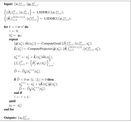
Figure 3: The mode-seeking algorithm in LSLDGC. LSDDR1({xi}ni=1)denotes the LSDDR
es-timator for the first-order density-derivative-ratios from data samples {xi}ni=1, and {βej}Dj=1 and {ci}bi=1 are the coefficients and (sub-sampled) centers, respectively.
ModeSeeking({βej}Dj=1,{ci}bi=1,zkτ) is a single step moseeking process whose
de-tails are given in Fig.4. The update ofzkτ terminates when eitherDb orkzkτ+1−zkτkis
less than a small positive constant.
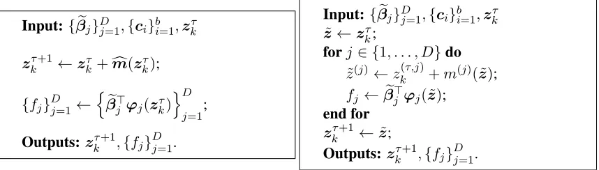
Input:{βej}Dj=1,{ci}bi=1,zτk
zkτ+1←zkτ+cm(zkτ);
{fj}Dj=1←
n
e
β>j ϕj(zkτ)
oD
j=1;
Outputs:zτk+1,{fj}Dj=1.
Input:{βej}Dj=1,{ci}bi=1,zτk
˜
z←zτ k;
forj∈ {1, . . . , D}do ˜
z(j)←zk(τ,j)+m(j)( ˜z); fj ←βej>ϕj( ˜z);
end for
zτk+1 ←z;˜
Outputs:zkτ+1,{fj}Dj=1.
Figure 4: Two mode-seeking algorithms in LSLDGC. The left figure uses the update rule (12), while the right one is based on the coordinate-wise update rule (15). ϕj(z) = (ϕ(1)j (z), ϕj(2)(z), . . . , ϕj(b)(z))>whereϕ(ji)(z) =ϕ
kz−cik2
2σ2
j
gradient ascent. SCMS obtains such a subspace as the span of the eigenvectors of the negative Hessian matrix of the log-density, which is called theinverse local-covariance matrix(Ozertem and Erdogmus, 2011):
Σ−1(x) :=−∇∇logp(x) =−∇∇p(x)
p(x) +
∇p(x)∇p(x)>
p(x)2 =−H(x) +g(x)g(x)
>.
(26)
An advantage of employing the log-density is discussed in the context of manifold estimation in Genovese et al. (2014): Theorem 7 in Genovese et al. (2014) states that when D-dimensional data is assumed to be generated on ad-dimensional manifold withD-dimensional Gaussian noise, the density ridge is close to the lower-dimensional manifold in the sense of the Hausdorff distance, and thus can be a surrogate for the manifold. This surrogate property holds in anO(1) neighbor-hood of the manifold for the log-density, while the theorem holds in anO(σn)neighborhood of the
manifold for the (non-log) density, whereσnis the standard deviation of the Gaussian noise.
Fur-thermore, whenp(x)is Gaussian, (26) reduces to the inverse of the covariance matrix. This allows us to intuitively understand that SCMS finds the subspace by PCA to the non-stationary covariance matrix at a locationxaround the ridge.
In practice, SCMS substitutespbKDE(x)into (26):
b
Σ−KDE1 (x) :=−∇∇pbKDE(x) b
pKDE(x)
+∇pbKDE(x)∇pbKDE(x)
>
b
pKDE(x)2
.
Then, SCMS obtains the orthogonal projector to the subspace as LbKDE(x) =
b
VKDE(x)VbKDE(x)>, where VbKDE(x) ∈ RD×(D−d) consists of the D −d eigenvectors
as-sociated with theD−dlargest eigenvalues ofΣb−KDE1 (x). Then, the update rule of SCMS is given
by
zτ+1 =zτ+LbKDE(zτ)cmKDE(zτ), (27)
wherezτ denotes theτ-th update of an arbitrarily initialized point andmcKDE(x)is the mean shift
vector defined in (10). Eq.(27) is repeatedly applied until convergence. The monotonic hill-climbing property for SCMS is proved in Ghassabeh et al. (2013).
One of the key challenges in SCMS is to accurately estimate Σ−1(x) in (26). SCMS takes a three-step approach, i.e., estimate p(x) by KDE, compute its derivatives, and plug them into
Σ−1(x). However, this approach can perform poorly because of the same reason as MS, i.e., a
good density estimator does not necessarily mean a good density derivative estimator. In addition, division by the estimated density could further magnify the estimation error for density derivatives. To cope with this problem, we employ LSDDR for direct estimation of density-derivative-ratios in
Σ−1(x) without going through density estimation and division, and propose a novel method for density ridge estimation.
4.3 Least-Squares Density Ridge Finder
Input:{xi}ni=1,{yk}n
0
k=1.
n
{βej}Dj=1,{ci}bi=1 o
←LSDDR1({xi}ni=1);
n
{θej}
D(D+1)/2
j=1 ,{c
0 i}bi=1
o
←LSDDR2({xi}ni=1);
fork= 1ton0do
τ ←0; zkτ ←yk; repeat
{gb(zτk),cm(z
τ
k)} ←ComputeGrad({βej}Dj=1,{ci}bi=1,zkτ); b
L(zkτ)←ComputeProjector(gb(z
τ k),{θbj}
D(D+1)/2
j=1 ,{c
0
i}bi=1,zkτ);
zτk+1 ←zkτ+Lb(zkτ)cm(zkτ);
{fj}Dj=1 ←
n
e
β>j ϕj(zkτ)
oD
j=1;
b
D←Db b
g[zkτ+1|zτk];
ifD <b 0or∃j, |fj| ≈0then
zkτ+1←zkτ +ηLb(zkτ)gb(zkτ); b
D←Db b
g[zkτ+1|zkτ]; end if
τ ←τ + 1;
until
zk←zkτ; end for
Outputs:{zk}n
0
k=1.
Figure 5: The algorithm of LSDRF. LSDDR2({xi}ni=1) denotes the LSDDR estimator for
the second-order density-derivative-ratios, and {θbj}
D(D+1)/2
j=1 are the corresponding
coefficient vectors. {yk}n
0
k=1 are initial points to approximate the density ridge.
ComputeGrad({βej}Dj=1,{ci}bi=1,zkτ)computes the estimated log-density gradientgb(zkτ)
and cm(z
τ
k) in (14), while ComputeProjector(gb(z
τ k),{θbj}
D(D+1)/2
j=1 ,{c
0
i}bi=1,zkτ)
com-putes the subspace projector Lb(zτk). The update of zkτ terminates when either Db or
4.3.1 ALGORITHM OFLSDRF
The algorithm of LSDRF essentially follows the same line as SCMS, which performs projected gradient ascent. By employing LSDDR, we obtain an estimate ofΣ−1(x)as
b
Σ−1(x) :=−Hc(x) +gb(x)gb>(x), (28)
where we recall thatbgj(x)and[Hc(x)]ij are LSDDR to∂jp(x)/p(x)and∂i∂jp(x)/p(x),
respec-tively. Then, we obtain the orthogonal projector to the subspace asLb(x) = Vb(x)Vb>(x) where b
V(x)consists of theD−deigenvectors associated with theD−dlargest eigenvalues ofΣb
−1
(x). By replacing LbKDE(x) and cmKDE(x) in (27) with Lb(x) and cm(x) respectively, the following
update rule for LSDRF is obtained by
zτ+1 =zτ+Lb(zτ)cm(zτ), (29)
where cm(x) = (mb(1)(x),mb(2)(x), . . . ,mb(D)(x))is used in LSLDGC for mode-seeking whose definition is given in (14).
The implementation techniques of LSLDGC in Section 3.4 are inherited, but LSDRF per-forms projected gradient ascent instead of the gradient ascent: Whenever Db
b
g[zτ+1|zτ] < 0 or
∃j, fj(z(τ))≈0, we perform the projected gradient ascent as
zτ+1 =zτ+ηLb(zτ)gb(zτ). (30)
The step size parameterηis selected so thatDb b
g[zτ+ηLb(zτ)bg(zτ)|zτ]is maximized. The algorithm
of LSDRF is summarized in Fig.5.4 The algorithm is essentially the same as LSLDGC based on the update rule (12) (Figs. 3 and 4), where we only replace (13) and (24) in LSLDGC with (29) and (30) in LSDRF, respectively. Unlike clustering, for density ridge estimation, the starting points zτ=0are arbitrary, but in this paper, we set them at data samplesxi because data samples are fairly
good starting points.
4.3.2 THECONVERGENCERATE TO THETRUERIDGE
Here, we establish the convergence rate to understand how the estimated ridge approaches to the true ridge asnincreases. Based on LSDDR, the estimated ridge is defined as
b
R:={x∈RD| kVb(x)Vb(x)>gb(x)k= 0,ηbd+1(x)<0},
whereηbi(x)denotes thei-th largest eigenvalue of−Σb−1(x).
In our analysis, we make the following assumptions:
(A0) Kernel boundedness: k(x,x0) and∂j∂j0k(x,x0)for all j are uniformly bounded, where ∂j0
denotes the partial derivative with respect to thej-th coordinate inx0.
(A1) Differentiability and boundedness: LetBD(x, δ)be theD-dimensional ball of radiusδ > 0
centered atxand letR ⊕δ:=∪x∈RBD(x, δ). For allx∈ R ⊕δ, the|j|-th order derivatives
oflogp(x)for|j|= 0,1,2,3exist and are bounded.
(A2) Eigengap: Assume that there existsκ >0andδsuch that for allx∈ R ⊕δ,ηd+1(x)<−κ
andηd(x)−ηd+1(x)> κ, whereηi(x)denotes thei-th eigenvalue of∇∇logp(x).
(A3) Path smoothness: For eachx∈ R ⊕δ,
kL⊥(x)g(x)k · kΣ−10(x)kmax<
κ2
2D3/2,
whereL⊥(x) :=ID−V(x)V(x)>,Σ−10(x) :=∇vec Σ−1(x)
, vec(·)denotes vectoriza-tion of matrices by concatenating the columns, andkAkmax := maxi,j|[A]ij|. The(i, j)-th
element in∇vec Σ−1(x)(∈RD2×D
)is given by∂j[vec Σ−1(x)
]i.
Assumptions (A2) and (A3) are a straightforward modification of the assumptions in Genovese et al. (2014) from the (non-log) density to the log-density. Assumption (A2) indicates that the density ridge has a sharp and curvilinear shape in the subspace orthogonal to the ridge. Assumption (A3) indicates thatkL⊥(x)g(x)kandkΣ−10(x)kmax are both bounded. SinceL⊥(x)is orthogonal to V(x)V(x)>for allx, the boundedness ofkL⊥(x)g(x)kimplies that the gradientg(x)is not too steep in the orthogonal subspace. The boundedness of kΣ−10(x)kmax means that the third-order derivative is bounded and thus the subspace direction does not abruptly change, which implies that the (projected) gradient ascent path cannot be too wiggly (Genovese et al., 2014, Section 2.2). Note that Assumptions (A1)-(A3) are only valid in the neighborhood around the ridge.
Let
0 := max
j kgj(x)−gbj(x)k∞,
00:= max ij k[Σ
−1(x)]
ij −[Σb
−1
(x)]ijk∞,
000 := max ij k[Σ
−10(x)] ij −[Σb
−10
(x)]ijk∞.
To establish the convergence rate, we rely on two lemmas. The first lemma is a simple modification of Theorem 4 in Genovese et al. (2014) to the log-density from the (non-log) density, and we use it without proof. The lemma states that if0, 00 and000 are sufficiently small, then the true and estimated ridges are close to each other:
Lemma 11 Suppose that (A1)-(A3) hold. Letψ := max{0, 00}andΨ := max{0, 00, 000}. When Ψis sufficiently small, the following statements hold:
(i) Conditions (A2) and (A3) hold forbg,Σb
−1
andΣb
−10 .
(ii) Haus(R,Rb)is bounded as
Haus(R,Rb) =O(ψ). (31)
The next lemma characterizes the convergence rates of0,00and000when we employ LSDDR:
Lemma 12 Suppose that the assumptions in Theorem 1 and (A0) hold. When LSDDR is applied for density-derivative-ratio estimation,
0 =OP
n−min
n 1 4,
γ
2(γ+1)
o
, (32)
00=OP
n−min
n 1 4,
γ
2(γ+1)
o
, (33)
000 =OP
n−min
n 1 4,
γ
2(γ+1)
o
The proof is given in Appendix G.
Combining Lemma 11 with Lemma 12 yields the following theorem:
Theorem 13 Suppose that the assumptions in Theorem 1 and (A0)-(A3) hold. Then,
Haus(R,Rb) =OP
n−min
n 1 4,
γ
2(γ+1)
o
. (35)
Proof Lemma 12 ensures thatψ =OP
n−min
n 1 4,
γ
2(γ+1)
o
. This completes the proof from (31).
Remark 14 Genovese et al. (2014, Eq.(1)) established the following convergence rate based on KDE:
Haus(R,RbKDE) =OP
logn n
2
D+8 !
, (36)
whereRbKDEdenotes the estimated ridge by KDE. Comparison to our result is difficult, but the main
difference is that the rate in(36)explicitly depends on data dimensionD.
5. Numerical Illustration on Mode-Seeking Clustering and Density Ridge Estimation
This section experimentally illustrates the performance of the proposed methods for mode-seeking clustering and density ridge estimation on a variety of datasets.
5.1 Illustration on Clustering
First, we illustrate the performance of LSLDGC both on artificial and benchmark datasets.
5.1.1 ARTIFICIALDATASETS: LSLDGCVSMS
Here, we compare the performance of LSLDGC to MS with two different bandwidth selection methods:
• LSLDGC: LSLDGC based on the update rule (12). The width parameterσj in the Gaussian
kernel and regularization parameterλjwere selected by cross-validation as in Section 2.4. We
selected ten candidates ofσj andλjfromcσ×σ
(j)
med(0.5≤cσ ≤5) and10m(−3≤m≤0),
respectively whereσ(medj) is the median value of|xi(j)−x(kj)|with respect toiandk.
• LSLDGCCW: LSLDGC based on the coordinate-wise update rule (15). The same
cross-validation was performed as above.
• MSLS: The bandwidth parameter h was cross-validated based on the standard integrated
squared error. We selected ten candidates ofhfrom10l×h
med(−1.5 ≤l≤0) wherehmed
• MSNR: The bandwidth parameterhwas determined by
¯
Sn
4
D+ 4
D1+6
n−d+61 ,
where S¯n = nD1 PDj=1Pni=1(x(ij)−x¯(j))2 andx¯(j) = n1Pni=1x(ij). This bandwidth
pa-rameter was used in Chen et al. (2016b) and a slight modification of the normal reference rule (Silverman, 1986).
First, we generated three kinds of two-dimensional data as follows:
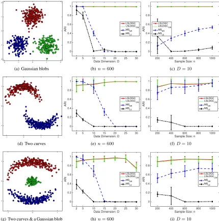
(a) Three Gaussian blobs(Fig.6(a)): Each data sample was drawn from a mixture of three Gaus-sians with means(0,1)>,(−1,−1)>and(1,−1)>, and covariance matrices0.1I2. The mixing
coefficients were0.4,0.3,0.3, respectively.
(b) Two curves (Fig.6(d)): Two curves are generated as (x(1), x(2)) = (cos(πt(1)),sin(πt(1)))>
and (x(1), x(2)) = (−cos(πt(2)) + 1,−sin(πt(2)))> where t(1) and t(2) are independently drawn from the Gaussian density with mean0.5and standard deviation0.15. Then, Gaussian noise with covariance matrix0.1I2was added to these curves. The numbers of data samples for
both curves were approximately same.
(c) Two curves & a Gaussian blob(Fig.6(g)): Data samples from the Gaussian density with mean
0 and standard deviation0.1were added to the two curves similarly generated as in (b). The number of samples for the two curves was same, and for the Gaussian blob, we set the number atn/3approximately.
When higher-dimensional data were generated, we simply appended Gaussian variables with mean
0and standard deviation 0.1to the two-dimensional data. Clustering performance was measured by the adjusted Rand index (ARI) (Hubert and Arabie, 1985): ARI takes a value less than or equal to one, a larger value indicates a better clustering result, and when a clustering result is perfect, the ARI value equals to one.
Fig.6(b,e,h) clearly indicates the advantage of our clustering methods over MS: Both LSLDGC and LSLDGCCW significantly outperform MSLS and MSNR particularly for higher-dimensional
data. When the dimensionality of data is low, MSNR performs well to all kinds of datasets.
How-ever, the ARI values of both MSLSand MSNRquickly approach zero as the dimensionality of data
increases. These unsatisfactory results seem to be due to the fact that the bandwidth selection in KDE is more difficult for high(er)-dimensional data. Thus, our direct approach would be more suitable particularly for high(er)-dimensional data.
Both LSLDGC and LSLDGCCW keep the ARI values high on a wide range of sample sizes
(Fig.6(c,f,i)). The performance of MSNR is improved as n increases. However, MSLS performs
rather worse for large(r) datasets. The least-squares cross-validation often suggests small bandwidth parameters for large(r) datasets, which make the estimated density unsmooth. Thus, the estimated density can include a lot of spurious modes with small peaks even if it was good in terms of density estimation. This also supports that our direct estimation is a more appropriate approach.
5.1.2 BENCHMARKDATASETS
-2 -1 0 1 2 -2 -1 0 1 2
(a) Gaussian blobs
2 5 10 15 20 25 30
Data Dimension: D 0 0.2 0.4 0.6 0.8 1 ARI LSLDGC LSLDGC CW MS NR MS LS
(b)n= 600
200 400 600 800 1000
Sample Size: n 0 0.2 0.4 0.6 0.8 1 ARI LSLDGC LSLDGCCW MSNR MSLS
(c)D= 10
-1 0 1 2
-1 0 1
(d) Two curves
2 5 10 15 20 25 30
Data Dimension: D 0 0.2 0.4 0.6 0.8 1 ARI LSLDGC LSLDGC CW MS NR MS LS
(e) n= 600
200 400 600 800 1000
Sample Size: n 0 0.2 0.4 0.6 0.8 1 ARI LSLDGC LSLDGCCW MSNR MSLS
(f) D= 10
-1 0 1
-1 0 1
(g) Two curves & a Gaussian blob
2 5 10 15 20 25 30
Data Dimension: D 0 0.2 0.4 0.6 0.8 1 ARI LSLDGC LSLDGC CW MS NR MS LS
(h)n= 600
200 400 600 800 1000
Sample Size: n 0 0.2 0.4 0.6 0.8 1 ARI LSLDGC LSLDGCCW MSNR MSLS
(i)D= 10
Table 1: The average and standard deviation of ARI values over50runs. A larger value means a better result. Numbers in the parentheses are standard deviations. The best and compa-rable methods judged by the unpaired t-test at the significance level1%are described in boldface.
Banknote(D, n, c) = (4,100,2)
LSLDGC LSLDGCCW MSLS MSNR SC KM
0.165(0.059) 0.169(0.055) 0.036(0.014) 0.167(0.147) 0.054(0.064) 0.039(0.051)
Accelerometry(D, n, c) = (5,300,3)
LSLDGC LSLDGCCW MSLS MSNR SC KM
0.628(0.058) 0.624(0.065) 0.029(0.007) 0.500(0.041) 0.226(0.271) 0.499(0.023)
Olive oil(D, n, c) = (8,200,9)
LSLDGC LSLDGCCW MSLS MSNR SC KM
0.717(0.081) 0.728(0.062) 0.020(0.019) 0.756(0.078) 0.552(0.060) 0.618(0.063)
Vowel(D, n, c) = (10,110,11)
LSLDGC LSLDGCCW MSLS MSNR SC KM
0.147(0.037) 0.139(0.032) 0.017(0.010) 0.133(0.026) 0.145(0.027) 0.180(0.027)
Sat-image(D, n, c) = (36,120,6)
LSLDGC LSLDGCCW MSLS MSNR SC KM
0.427(0.072) 0.422(0.073) 0.000(0.000) 0.343(0.063) 0.418(0.056) 0.434(0.052)
Speech(D, n, c) = (50,400,2)
LSLDGC LSLDGCCW MSLS MSNR SC KM
0.146(0.063) 0.147(0.054) 0.000(0.000) 0.000(0.000) 0.004(0.004) 0.002(0.004)
• Banknote(D= 4, n= 100, andc= 2)(Bache and Lichman, 2013)5: This dataset consists of four-dimensional features from400by400images for genuine and forged banknote-like specimens. The features were extracted by wavelet transformation. We randomly chose50
samples from each of the two classes.
• Accelerometry(D = 5, n = 300, andc = 3)6: The ALKAN dataset contains3-axis (i.e., x-, y-, and z-axes) accelerometric data. During the data collection, subjects were instructed to perform walking, running, and standing up. After segmenting each data stream into windows, five orientation-invariant-features were computed from each window (Sugiyama et al., 2014). We randomly chose100samples from each of the three classes.
• Olive oil(D= 8, n= 200, andc= 9)(Forina et al., 1983). This dataset was obtained from the R software.7 The dataset includes eight chemical measurements on different specimen of olive oil produced in nine regions in Italy. We randomly chose200samples.
• Vowel(D = 10, n = 110, and c = 11)(Turney, 1993; Bache and Lichman, 2013)8: This consists utterance data for eleven vowels of British English. Each utterance is expressed by a ten-dimensional vector. We randomly chose10samples from each of the eleven classes.
• Sat-image(D= 36, n= 120, andc= 6)(Bache and Lichman, 2013)9: The dataset contains the multi-spectral values of pixels in3×3neighborhoods in a satellite image with six classes. We randomly chose20samples from each of the six classes.
• Speech (D = 50, n = 400, and c = 2). An in-house speech dataset (Sugiyama et al., 2014), which contains short utterance samples recorded from2 male subjects speaking in French with sampling rate44.1kHz. 50-dimensional line spectral frequencies vectors (Kain and Macon, 1998) were computed from each utterance sample. We randomly chose 200
samples from each of the two classes.
As preprocessing, each data sample was standardized by the sample mean and standard deviation in coordinate-wise manner. For comparison, we appliedk-means clustering(KM) (MacQueen, 1967) andspectral clustering(SC) (Ng et al., 2001; Shi and Malik, 2000) to the same datasets. Since KM and SC require to input the number of clusters, we set it at the correct number.
As seen in the illustration on artificial data, when the dimensionality of data is low, the perfor-mance of LSLDGC, LSLDGCCW and MSNR is comparable, but LSLDGC and LSLDGCCW
sig-nificantly work better than MSNRto higher-dimensional datasets (sat-image and speech datasets).
KM and SC have prior information about the number of clusters. Nonetheless, the performance of LSLDGC and LSLDGCCWare often better than KM and SC.
From the results of both the artificial and benchmark datasets, we conclude that LSLDGC and LSLDGCCWare advantageous to relatively high-dimensional data.
5.2 Illustration on Density Ridge Estimation
Next, we illustrate the performance of LSDRF, and compare LSDRF with SCMS both on artificial and standard benchmark datasets.
5.2.1 ARTIFICIALDATA: LSDRFVSSCMS
The performance of LSDRF is compared to SCMS with two different bandwidth selection methods:
• LSDRF: When estimatinggj(x), we selected ten candidates of the width parameter in the
Gaussian kernel and the regularization parameter from 10l ×σ(medj) (−0.3 ≤ l ≤ 1) and
10m (−4 ≤ m ≤ 0), respectively. When estimating[H(x)]ij, ten candidates of the width
parameter in the Gaussian kernel were selected from10l×
q
σmed(i) σ(medj) (−0.3≤l≤1). For the regularization parameter, we used the same candidates as ingj(x).
7.https://artax.karlin.mff.cuni.cz/r-help/library/pdfCluster/html/oliveoil.html 8.https://archive.ics.uci.edu/ml/datasets/Connectionist+Bench+(Vowel+
Recognition+-+Deterding+Data)
data True LSDRF
data True SCMS
LS
data True SCMS
CR
data True LSDRF
(a) LSDRF
data True SCMS
LS
(b) SCMSLS
data True SCMS
CR
(c) SCMSCR
Figure 7: Comparison of the two estimated ridges by LSDRF, SCMSLSand SCMSCR.
• SCMSLS: The bandwidth parameterh was cross-validated based on the standardintegrated
squared error. We selected ten candidates ofhfrom10l×hmed(−1.5 ≤l≤0) wherehmed
is the median value of|x(ij)−xk(j)|with respect toi,jandk.
• SCMSCR: The bandwidth parameter hwas cross-validated based on the coverage risk
pro-posed in Chen et al. (2015a). As suggested in Chen et al. (2015a), we selected ten candidates ofhfrom10l×h
NR(−1≤l≤0) wherehNRis the bandwidth based on the normal reference
rule (Silverman, 1986).
We investigate the performance of these methods on a variety of simulated datasets.10 The i-th observation of data was generated according to x(ij) = f(j)(ti) +n(ij), whereti was taken from
some range at regular intervals,f(j)(·)denotes some fixed function, andn(ij)was the Gaussian noise with mean0and standard deviation0.15. Higher-dimensional data were created by appending the Gaussian variables with mean0and standard deviation0.15. The estimation error was measured by
Error= 1
n
n
X
i=1
min
l kybi−f(tl)k, (37)
wheref(·) = (f(1)(·), f(2)(·), . . . , f(D)(·))>andybidenotes an estimate of the density ridge point
fromxi.
data SCMS LS SCMS CR LSDRF
200 400 600 800 1000
Sample Size: n 0.03 0.06 0.09 Error LSDRF SCMSLS SCMSCR
6 9 12 15
Data Dimension: D 0 0.2 0.4 0.6 Error LSDRF SCMS LS SCMS CR data SCMS LS SCMS CR LSDRF
200 400 600 800 1000
Sample Size: n 0.04 0.08 0.12 Error LSDRF SCMSLS SCMSCR
6 9 12 15
Data Dimension: D 0 0.2 0.4 0.6 Error LSDRF SCMSLS SCMSCR data SCMS LS SCMS CR LSDRF
200 400 600 800 1000
Sample Size: n 0 0.04 0.08 Error LSDRF SCMSLS SCMSCR
6 9 12 15
Data Dimension: D 0 0.2 0.4 0.6 Error LSDRF SCMSLS SCMSCR data SCMS LS SCMS CR LSDRF
200 400 600 800 1000
Sample Size: n 0.04 0.08 Error LSDRF SCMSLS SCMSCR
6 9 12 15
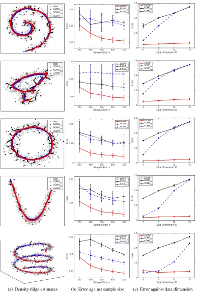
Data Dimension: D 0 0.2 0.4 0.6 Error LSDRF SCMSLS SCMSCR
(a) Density ridge estimates
200 400 600 800 1000
Sample Size: n 0.05 0.1 0.15 Error LSDRF SCMSLS SCMSCR
(b) Error against sample size
6 9 12 15
Data Dimension: D 0 0.2 0.4 0.6 Error LSDRF SCMSLS SCMSCR
(c) Error against data dimension
The estimated ridges are visualized in Fig.7. SCMSLSprovides a broken and non-smooth ridge
estimate because the selected bandwidth by the least-squares cross-validation is small for density ridge estimation as in mode-seeking clustering. In contrast, the ridges estimated by LSDRF and SCMSCRare smooth. However, SCMSCR gives a biased estimate around highly curved region in
the true ridge (e.g., the centers of the spiral and quadratic curve in Fig.7), while the bias in LSDDR seems smaller. This implies that LSDRF more accurately estimates density ridges. The accuracy of LSDRF is quantified on a variety of artificial datasets in Fig 8. LSDRF produces smaller errors particularly when the sample size is large (Fig 8(b)). In addition, as in mode-seeking clustering, the performance of LSDRF is even better when the dimensionality of data is higher (Fig. 8(c)). This implies that our direct approach is useful for high(er)-dimensional data.
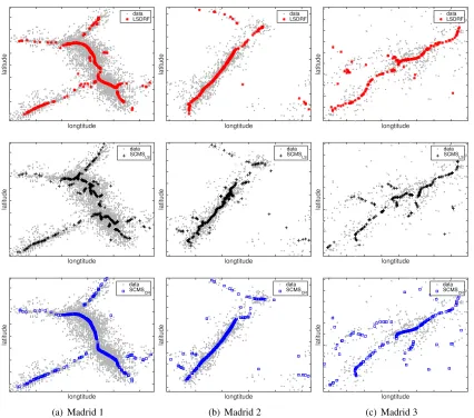
5.2.2 DENSITYRIDGEESTIMATION ONREAL-WORLDDATASETS
Next, we apply LSDRF to real-world datasets. As in Pulkkinen (2015), we employed the following two datasets:
• New Madrid earthquakedataset: This seismological dataset was downloaded from the Center for Earthquake Research and Information.11 The dataset contains positional information for earthquakes around the New Madrid seismic zone from1974to2016, providing11,131 sam-ples. The three regions in Figs.9(a,b,c) were extracted according to (a)(−90.2,−89.25), (b)
(−92.5,−92.15)and (c)(−85.5,−83.5)degrees for the latitude range, respectively. For the longitude range, (a)(36,36.8), (b)(35.2,35.4)and (c) (34.5,36.5)degrees were selected. The total numbers of the original data samples and reduced data samples in each region were (a)(N, n) = (5902,500), (b)(N, n) = (1548,300)and (c)(N, n) = (594,200).
• Shapley galaxy dataset: This dataset was downloaded from the Center for Astrostatis-tics at Pennsylvania State University.12 The dataset contains information about the three-dimensional sky angles and recession velocity of 4,215 galaxies. As done in Pulkkinen (2015), we transformed the data samples into the three-dimensional Cartesian coordinates based on the fact that the recession velocity is proportional to the radial distance (Drinkwater et al., 2004). The three regions in Figs 10(a,b,c) were extracted according to a velocity range: (a)(6000,20000)km/s, (b)(1500,6000)km/s and (c)(6000,10500)km/s, respectively. The total numbers of the original data samples and reduced data samples in each region were (a)
(N, n) = (2849,500), (b)(N, n) = (595,200)and (c)(N, n) = (351,150).
In each dataset, we focused on three regions containing prominent features, and standardized data samples in each region by subtracting the mean value and dividing by standard deviation in a dimension-wise manner. Here, the standardized data samples are collectively denoted by
e
D = {xei}Ni=1. Before applying density ridge estimation methods, we performed preprocessing
to remove clutter noises: KDE was applied to the dataset of each region, and then the data samples
e
xi in each region were removed when maxpbjKDE[ (xei)
b
pKDE(xej)]
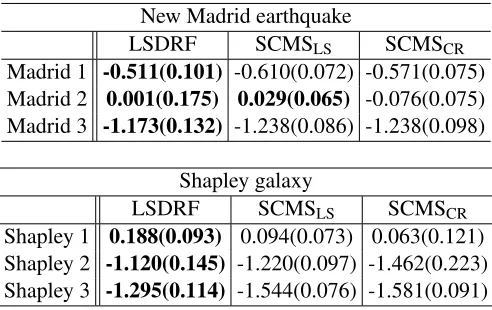
< 10−3. After noise removal, we randomly chosendata samples from each region, and applied the three density ridge estimation methods to the sub-sampled data. The sub-sampled data are collectively expressed byD= {xi}ni=1. For
per-formance comparison, we computed the logarithm ofpbKDEon the estimated density ridges, which 11.http://www.memphis.edu/ceri/seismic/